$\pi K$ scattering inputs to ChPT

Abstract

Experimental information on low energy $\pi K$ scattering would shed light on the poorly known OZI suppressed sector of ChPT. I describe recent work aimed at generating such information based on available experimental data by setting up and then solving with appropriate boundary conditions a non linear system of equations of the Roy and Steiner type. First results of this analysis are presented.

This talk describes work done with Paul Büttiker and Sébastien Descotes-Genon. Following ideas and methods due to Roy[1] and to Steiner[2], our aim was to generate data on the $\pi K$ scattering amplitude at very low energy, even in unphysical regions, using input experimental data at medium and high energy. I will begin by explaining the need for such $\pi K$ data in connection with developments of ChPT and questions about different chiral limits.

The fundamental degrees of freedom of QCD are quarks and gluons. Because the three lightest quarks happen to have masses much smaller than 1 GeV it is possible, in a limited kinematical region of the non perturbative regime, to make a change of variables and use an effective Lagrangian where $\pi$, $K$ and $\eta$ are the fundamental degrees of freedom. This Lagrangian allows one to perform expansions around chiral limits. There are two different chiral limits which are relevant to the physical world: one with $N^{0}_{F}=2$ massless flavours and one with $N^{0}_{F}=3$. The chiral Lagrangian at order $p^{4}$ (NLO) was constructed by Gasser and Leutwyler[3] and involves 10 independent coupling constants $L_{i}$. More recently, the chiral Lagrangian at NNLO was constructed[4] which brings in a number of new couplings $C_{i}$. It becomes of obvious importance to collect as much experimental data as possible to test the theory. The pion-Kaon scattering amplitude turns out to be a particularly interesting process in connection with ChPT. The computation of the amplitude at order $p^{4}$ was performed in ref.[5]. By matching this expression with low energy experimental input allows one to probe many of the chiral couplings including those which are suppressed in the large $N_{c}$ limit, like the coupling $L_{4}$ [6]. Such couplings ($L_{4}$, $L_{6}$ and the combination $L_{2}-2L_{1}$ ) were set equal to zero (and a plausible guess of the error was made) in the original work or ref.[3]. Their actual values have interesting physical implications. For instance, the value of $F_{\pi}$ in a chiral limit is an order parameter for the spontaneous breaking of chiral symmetry. The coupling $L_{4}$ controls the difference in the values of $F_{\pi}$ in the chiral limits with $N^{0}_{F}=2$ and $N^{0}_{F}=3$. This difference is a non trivial dynamical property of QCD which is linked to the puzzling properties of the light scalar mesons. An unrealistic but amusing illustration of this link is provided by the “extended” linear sigma model discussed in ref.[7]: for certain scalar meson assignments a dramatically large change in $F_{\pi}$ is predicted. The low energy $\pi K$ amplitude probes not only $L_{4}$ but also to some extent $L_{6}$ (via the combination $L_{8}+2L_{6}$ ) and also several other chiral coupling constants.

Experimental data on the $\pi K$ amplitude at sufficiently low energies are either unavailable or unreliable but one can construct such data based on reliable experimental input. Such a construction is made possible because the S-matrix has analyticity properties, from which one can write down dispersion relations. Next, the property of crossing allows one to determine the subtraction functions. What makes the pseudo-scalar mesons unique in the application of these methods is that they are the lightest particles in the QCD spectrum. As a consequence, scattering of pseudo-scalar mesons is elastic at low energies. In practice, there exists a significant energy region ($E\mathrel{\raise 2.58334pt\hbox{$<$}\kern-7.7778pt\lower 2.79857pt\hbox{$\sim$}}$ 1 GeV ) in which scattering can be considered as elastic to a very good approximation. Finally, in this same region the partial waves with $l\geq 2$ are negligibly small such that after projecting the dispersion relations over partial waves one obtains a closed system of equations for the S and the P waves in the energy region $E\leq E_{m}$ (with $E_{m}\simeq$ 1 GeV is called the matching point). The amplitude for $E\geq E_{m}$ must be provided as input to these equations. Such equations were first proposed by Roy[1] (for $\pi\pi$ scattering) and by Steiner[2]. While $\pi\pi$ scattering was intensively studied (see e.g.[8] and references therein), much less work was devoted to $\pi K$. Also, in earlier work[9, 10, 11] no accurate experimental input data was available. In the $\pi K$ case, one can derive a set of six coupled equations which involve the four partial waves $f_{0}^{I}$,$f_{1}^{I}$ with $I={1\over 2},\ {3\over 2}$ of the $\pi K\to\pi K$ amplitude and the two partial waves $g_{0}^{0}$, $g_{1}^{1}$ of the $\pi\pi\to K\overline{K}$ amplitude. These equations contain two arbitrary parameters which are conveniently chosen to be the two S-wave scattering lengths, $a_{0}^{1/2}$, $a_{0}^{3/2}$. A typical equation is shown below

$${\color[rgb]{0,0.6,0}Ref_{l}^{1\over 2}(s)}=k^{1\over 2}_{l}({\color[rgb]{1,0,0}a_{0}^{1/2},a_{0}^{3/2}},s)+{1\over\pi}\hbox{$-$}\kern-3.66667pt\hbox{$\displaystyle\int_{{m^{2}_{+}}}^{\infty}$}ds^{\prime}\,\sum_{l^{\prime}=0,1}$$

$$\Bigg{\{}\left(\delta_{ll^{\prime}}{\lambda_{s}\over(s^{\prime}-s)\lambda_{s^{\prime}}}-{1\over 3}K^{\alpha}_{ll^{\prime}}(s,s^{\prime})\right){\color[rgb]{0,0.6,0}{\rm Im}\,f_{l^{\prime}}^{1\over 2}(s^{\prime})}$$

$$+{4\over 3}K^{\alpha}_{ll^{\prime}}(s,s^{\prime}){\color[rgb]{0,0.6,0}{\rm Im}\,f_{l^{\prime}}^{3\over 2}(s^{\prime})}\Bigg{\}}+{1\over\pi}\int_{4m^{2}_{\pi}}^{\infty}dt^{\prime}$$

$$\Big{\{}K^{0}_{l0}(s,t^{\prime}){\color[rgb]{1,0,1}{\rm Im}\,g_{0}^{0}(t^{\prime})}+2K^{1}_{l1}(s,t^{\prime}){\color[rgb]{1,0,1}{\rm Im}\,g_{1}^{1}(t^{\prime})}\Big{\}}$$

$$+d^{1\over 2}_{l}(s)$$ (1)

which displays the usual singular Cauchy kernel and other non-singular kernels. Elastic unitarity provides an additional non-linear relation between real an imaginary parts.

Important progress was achieved recently by Gasser and Wanders[12] in clarifying the multiplicity properties of the Roy equations solutions. The $\pi K$ equations can be recast in a form analogous to that considered in ref.[12] after eliminating $g_{0}^{0}$, $g_{1}^{1}$. The multiplicity index is controlled by the values of the $\pi K$ phase shifts at the matching point. At the matching point, appropriate boundary conditions must be enforced: firstly, one must impose that the phase shifts are continuous. In practice this condition cannot be applied to $\delta_{1}^{3/2}$ which is too small and inaccurately measured at the matching point. This P-wave must be treated on the same footing as the $l\geq 2$ partial waves and does not influence the multiplicity index. Choosing the matching point to be at 1 GeV approximately, the multiplicity index turns out to vanish. This implies that for a given set of values for $a_{0}^{1/2},a_{0}^{3/2}$ if a solution exists, then it is unique. Two additional physical requirements that one can impose are that the derivatives of two of the phase shifts should also be continuous. These additional constraints can no longer be satisfied for arbitrary values of $a_{0}^{1/2},a_{0}^{3/2}$. If the input data were perfect, the S wave scattering lengths would be exactly determined as discrete eigenvalues of the system of Roy-Steiner (RS) equations together with the appropriate boundary conditions. Our work has consisted in determining how the S wave scattering lengths are constrained in practice from the available experimental data and their errors.

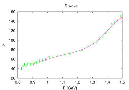
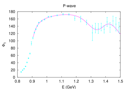
Figure 1: Input data for the $I=1/2$ S- and P-waves.

Let us now examine the experimental input data. In our analysis, we have used the experimental data for $\pi K\to\pi K$ from Estabrooks et al.[13] and from Aston et al.[14] which are both high statistics production experiments considerably more accurate than the data which were available before. We also need data on the $\pi\pi\to K\overline{K}$ amplitudes. For these, we have used the results from Cohen et al.[15] and from Etkin et al.[16] which are also generated from high-statistics production experiments. We note that the amplitudes in the unphysical region below the $K\overline{K}$ threshold are generated from solving the RS equations. Fig. 1 displays the data for the $\pi K$ S- and the P-waves it shows that the data are rather smooth and accurate in the region of the matching points. In order to ascertain the values of the phases and of the derivatives at the matching point (which are crucial in that analysis) we have performed several different types of fits. We use much more input than showed here: like higher partial waves, Regge models for asymptotic regions etc… more details will be provided in a forthcoming publication. The RS equations are then solved to high numerical accuracy.

The errors on the output of the equations are estimated by varying the parameters used in the fits to the input data and making use of their correlation matrices.

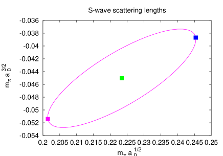
Figure 2: One-sigma ellipse for the two S-wave scattering lengths obtained by solving the RS equations with appropriate boundary conditions.

The main result of this analysis is the determination of a region inside which the two S-wave scattering lengths are constrained. This one-sigma ellipse is shown in Fig. 2. This result is rather non trivial as no experimental data at all has been used below one GeV ! As one can see from the figure, this region is rather small: this is a direct reflection of the precision of the data used as input, in particular in the region of the matching point.

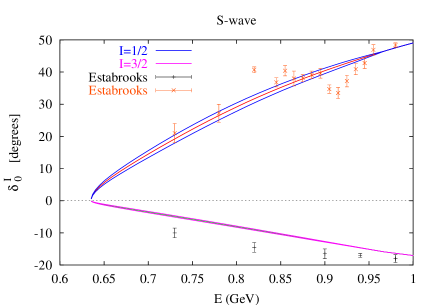
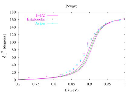
Figure 3: Results for S and P-wave phase-shifts in the low energy region obtained from solving the RS equations.

Fig. 3 shows phase shifts that we obtain from solving the RS equations. We display in every case three solutions corresponding to the three points in the $a_{0}^{1/2}$ $a_{0}^{3/2}$ plane as shown in Fig. 2. We also show for comparison some of the experimental data available in this region. A priori, the determination of the phase shifts from production experiments become less reliable at lower energies. In general, our results are not in very good agreement with the data in this region. The most striking disagreement concerns the P-wave. Our prediction for the mass of the $K^{*}$ is higher by 10 MeV than the mass from refs.[13, 14]. One possible reason for this discrepancy is isospin breaking which is not properly taken into account in our analysis but we also note that CLEO has reported a discrepancy between the mass of the $K^{*+}$ found in $\tau\to\pi K_{S}\nu$ decays and the PDG value[17].

Using the results of our work we can calculate the $\pi K$ amplitude at the threshold or below the threshold and match with ChPT expansions. These results will be presented elsewhere. In the future, we expect new data to become available which would help sharpen our predictions. Better data on the P-wave phase shift from CLEO is one example. Reliable data on the S-wave phase shifts could be provided from the $D$ decay mode $D\to\pi K\mu\nu$. Finally, $\pi K$ atom experiments are planned which could directly access combinations of scattering lengths.

References

- [1] S. M. Roy, Phys. Lett. B 36 (1971) 353.
- [2] F. Steiner, Fortsch. Phys. 19 (1971) 115.
- [3] J. Gasser and H. Leutwyler, Nucl. Phys. B 250 (1985) 465.
- [4] J. Bijnens, G. Colangelo and G. Ecker, Annals Phys. 280 (2000) 100 [hep-ph/9907333]; JHEP 9902 (1999) 020 [hep-ph/9902437].
- [5] V. Bernard, N. Kaiser and U. G. Meißner, Phys. Rev. D 43 (1991) 2757, Nucl. Phys. B 357 (1991) 129.
- [6] B. Ananthanarayan and P. Büttiker, Eur. Phys. J. C 19 (2001) 517 [hep-ph/0012023], B. Ananthanarayan, P. Buttiker and B. Moussallam, Eur. Phys. J. C 22 (2001) 133 [hep-ph/0106230].
- [7] B. Moussallam, JHEP 0008 (2000) 005 [hep-ph/0005245].
- [8] B. Ananthanarayan, G. Colangelo, J. Gasser and H. Leutwyler, Phys. Rept. 353 (2001) 207 [hep-ph/0005297].
- [9] J. P. Ader, C. Meyers and B. Bonnier, Phys. Lett. B 46 (1973) 403.
- [10] C. B. Lang, Nuovo Cim. A 41 (1977) 73.
- [11] N. Johannesson and G. Nilsson, Nuovo Cim. A 43 (1978) 376.
- [12] J. Gasser and G. Wanders, Eur. Phys. J. C 10 (1999) 159 [hep-ph/9903443], G. Wanders, Eur. Phys. J. C 17 (2000) 323 [hep-ph/0005042].
- [13] P. Estabrooks, R. K. Carnegie, A. D. Martin, W. M. Dunwoodie, T. A. Lasinski and D. W. Leith, Nucl. Phys. B 133 (1978) 490.
- [14] D. Aston et al., Nucl. Phys. B 296 (1988) 493.
- [15] D. Cohen, D. S. Ayres, R. Diebold, S. L. Kramer, A. J. Pawlicki and A. B. Wicklund, Phys. Rev. D 22 (1980) 2595.
- [16] A. Etkin et al., Phys. Rev. D 25 (1982) 1786.
- [17] J. Urheim [CLEO Collaboration], Nucl. Phys. Proc. Suppl. 55C (1997) 359.