THE SPECTRAL QUARK MODEL AND LIGHT-CONE PHENOMENOLOGY

Abstract

Chiral quark models offer a practical and simple tool to describe covariantly both low and high energy phenomenology in combination with QCD evolution. This can be done in full harmony with chiral symmetry and electromagnetic gauge invariance. We review the recently proposed spectral quark model where all these constraints are implemented.

1 INTRODUCTION

Light cone hadron properties provide a non-trivial playground to test ideas and methods on genuine non-perturbative QCD phenomenology. As we have heard from S. Brodsky in this workshop this information is conveniently encoded in LC wave functions [2]. They are measured through high energy inclusive, such as Deep Inelastic Scattering (DIS), or exclusive processes, which with the help of QCD renormalization group evolution can be related to low-energy matrix elements. In the particularly interesting case of the pion one expects chiral symmetry to impose certain constraints. The specific and general way how this is done seems unclear at the moment, because by asking about the quark content of a hadron we are actually in a situation where both hadrons and quarks coexist as degrees of freedom, so standard effective field theory tools like Chiral Perturbation Theory [3] do not apply directly beyond predicting finite pion mass corrections. On the other hand, fundamental lattice approaches naturally formulated in Euclidean space can only obtain low moments of structure functions (see e.g. the talk of P. E. L. Rakow and Ref. [4]) and distribution amplitudes, which are not testable directly through experiment. As B. van de Sande presented in his talk, QCD transverse lattice approaches can be directly formulated on the light-cone and although promising results for the pion and other mesons exist already [5] (for a review see e.g. Ref. [6]) they do not easily accommodate for chiral symmetry. The Schwinger-Dyson approach in its Euclidean formulation and its implications [7] has been reviewed by C. D. Roberts.

In order to gather some theoretical insight on the role of chiral symmetry in high energy inclusive [8] or exclusive [9] processes we remain at the more modest level of the so-called quiral quark models reviewed in Ref. [10]. This generic name stands for phenomenological relativistic quantum field theories where chiral symmetry is spontaneously broken incorporating Goldstone’s theorem. One of the advantages of such an approach is that it is covariant, so we avoid from the beginning the difficult marriage between light-cone quantization and chiral symmetry. In this talk we review salient features of recent work done by us on a new chiral quark model: the spectral quark model (SQM) [11, 12, 13]. This model shares many good aspects of other chiral models, particularly NJL type models, but improves others at a very low computational cost and, up to now, brings very encouraging phenomenological success.

QCD is a theory of quarks and gluons as elementary degrees of freedom, so both contribute to the total momentum carried by a hadron. The separation between gluons and valence and sea quarks, however, is both scale and renormalization scheme dependent which can be worked out explicitly within perturbative QCD. On the other hand, chiral quark models which are supposedly a low energy approximation to QCD, obviously saturate the momentum sum rule, since they contain no explicit gluonic degrees of freedom. This poses the natural question: is there any scale in QCD at which the momentum fraction carried by the (valence) quarks is exactly one ?

According to the phenomenological QCD analysis undertaken by the Durham group over a decade ago [14], the momentum fraction carried by the valence quarks is 0.47 $\%$ at the scale $\mu^{2}=4{\rm GeV}^{2}$, e.g., for $\pi^{+}$,

$$V_{1}(\mu)=\langle x\left(u_{\pi}-\bar{u}_{\pi}+\bar{d}_{\pi}-d_{\pi}\right)\rangle=0.47\pm 0.02\qquad{\rm at}\qquad\mu^{2}=4{\rm GeV}^{2}\;.$$ (1)

where $u_{\pi}$, $\bar{u}_{\pi}$ , $d_{\pi}$ and $\bar{d}_{\pi}$ are parton distribution functions (PDF) in the pion. Assuming LO perturbative QCD evolution one gets

$$\frac{V_{1}(\mu)}{V_{1}(\mu_{0})}=\left(\frac{\alpha(\mu)}{\alpha(\mu_{0})}\right)^{\gamma_{1}^{\rm NS}/2\beta_{0}}\quad,\qquad\alpha(\mu)=\left(\frac{4\pi}{\beta_{0}}\right)\frac{1}{\log(\mu^{2}/\Lambda_{\rm QCD}^{2})}$$ (2)

where $\gamma_{1}^{\rm NS}/2\beta_{0}=32/81$ for $N_{F}=N_{c}=3$. We take for concreteness $\Lambda_{\rm QCD}=226~{}{\rm MeV}$, which for $\mu=2{\rm GeV}$ yields $\alpha=0.32$. Downward LO evolution yields that for the reference scale, $\mu_{0}$,

$$V_{1}(\mu_{0})=1,\qquad\mu_{0}=313_{-10}^{+20}{\rm MeV}$$ (3)

Although this seems a rather low scale, one may still hope that the expansion parameter $\alpha(\mu_{0})/2\pi\sim 0.34\pm 0.04$ makes perturbation theory meaningful. A NLO analysis confirms this, at first glance “illegal”, expectation. This is the natural scale where all observables are defined in the quark model. If we want to compute observables at higher scales $\mu>\mu_{0}$ one may use QCD (perturbative) evolution using the quark model as an initial condition. This way we generate the missing (perturbative) gluon components explicitly in the form of QCD radiative corrections.

2 THE SPECTRAL QUARK MODEL

The subject of regularization in connection with high energy hadronic properties in chiral quark models has always been tricky and frustrating in the past, particularly when chiral and electromagnetic invariance, anomalies and factorization were demanded simultaneously (See Ref. [10] and references therein for a comprehensive discussion). The SQM relies on a spectral regularization of the chiral quark model proposed in Ref. [11] and extensively developed in Ref. [12] and is based on a generalized Lehmann representation for the quark propagator

$$S({p})=\int_{C}d\omega{\rho(\omega)\over\hbox to0.0pt{\hbox to5.03125pt{\hfil/\hfil}\hss}p-\omega}=\int_{C}d\omega\frac{\rho_{V}(\omega)\hbox to0.0pt{\hbox to5.03125pt{\hfil/\hfil}\hss}p+\rho_{S}(\omega)\omega}{p^{2}-\omega^{2}}=\frac{Z(p^{2})}{\hbox to0.0pt{\hbox to5.03125pt{\hfil/\hfil}\hss}p-M(p^{2})},$$ (4)

where $C$ is a general contour to be determined. For obvious reasons $\omega$ is called the spectral quark mass. Chiral and flavour gauge invariance on the relevant vertex functions are obtained (up to transverse terms) by means of the gauge technique of Delbourgo and West [15] which is nothing but minimal coupling at the spectral quark level. According to the analysis of Refs. [11, 12], the proper normalization and finiteness of hadronic observables are achieved by requesting a set of spectral conditions for the moments of the quark spectral function, $\rho(\omega)$, namely

$$\rho_{n} \equiv\int d\omega\omega^{n}\rho(\omega)=\delta_{n0},\;\;\;{\rm for}\;n=0,1,2,3,...$$ (5)

Physical observables turn out to be proportional to the inverse moments,

$$\rho_{-k} \equiv\int d\omega\omega^{-k}\rho(\omega),\;\;\;{\rm for}\;k=1,2,3,...$$ (6)

as well as to the so called “log moments”,

$$\rho^{\prime}_{n}\equiv\int d\omega\log(\omega^{2}/\mu^{2})\omega^{n}\rho(\omega)=\int d\omega\log(\omega^{2})\omega^{n}\rho(\omega),\;\;\;{\rm for}\;n=2,3,4,...$$

Note that the conditions (5) remove the dependence on the scale $\mu$ in (2), thus we can drop it from the log. Using these conditions one may prove a number of important features, like fulfillment of chiral anomalies and factorization of form factors, i.e. power like behaviour, in the high momentum limit. The main assumption in Eq. (4) is that of analyticity in the complex plane but not of positivity, since then even moments would not vanish for a positive spectral function. Analyticity enables direct calculations of hadron properties in the Minkowski space, an extremely convenient circumstance when doing light-cone physics. The analyticity assumption is also necessary in models formulated in Euclidean space, although the practical continuation to Minkowski may become numerically messy.

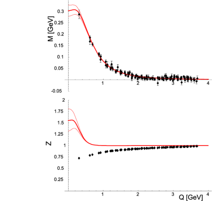
Figure 1: The dependence of the quark mass $M$ (top) and the wave function normalization $Z$ (bottom) on the Euclidean momentum $Q$ obtained from the meson dominance model with $d_{S}=5/2$. Lattice data from Ref. [17].

Although many results of our model do not depend on a particular choice of functions fulfilling the spectral conditions (5), a particular realization embodies more predictions. The standard approach to quark models is to assume a “reasonable” form for the quark propagator and work out hadronic properties from there. This poses the natural and difficult problem as to what is a reasonable spectral function. Out of ignorance we take a radically different approach, namely we deduce the spectral function from phenomenology. Actually, $\rho_{V}(\omega)$, can be uniquely deduced from the pion electromagnetic form factor, which for simplicity is assumed to be of the vector dominance monopole form. The net result [12] is the meson dominance (MD) model explicit realization which fulfills the above spectral conditions and is given by

$$\rho_{V}(\omega) = \frac{1}{2\pi i}\frac{1}{\omega}\frac{1}{(1-4\omega^{2}/M_{V}^{2})^{d_{V}}},\qquad\rho_{S}(\omega)=\frac{1}{2\pi i}\frac{16(d_{S}-1)(d_{S}-2)\rho^{\prime}_{3}}{M_{S}^{4}(1-4\omega^{2}/M_{S}^{2})^{d_{S}}},$$ (7)

The preferred values are $d_{V}=d_{S}=5/2$ and $M_{V}=776{\rm MeV}$ corresponds to the $\rho$-meson mass. The contour $C$ encircles the branch cuts, i.e., starts at $-\infty+i0$, goes around the branch point at $-m_{\rho}/2$, and returns to $-\infty-i0$, with the other section obtained by a reflexion with respect to the origin [12]. Straightforward calculation yields

$$\frac{M(p^{2})}{M(0)} = \frac{4d_{V}p^{2}}{M_{V}^{2}}\frac{\left(\frac{M_{S}^{2}}{M_{S}^{2}-4p^{2}}\right)^{d_{S}}}{\left(\frac{M_{V}^{2}}{M_{V}^{2}-4p^{2}}\right)^{d_{V}}-1}$$ (8)

Remarkably, when $M(p^{2})=p^{2}$ then $Z(p^{2})=0$ so that the quark propagator has no pole. Instead it has cuts at $p^{2}=M_{V}^{2}/4$. These feature is usually called analytic confinement and the rationale for it has been described in detail in Ref. [12]. A fit to the recent QCD lattice simulation in Landau gauge [17] yields $M(0)=303\pm 24~{}{\rm MeV}$ and $M_{S}=970\pm 21~{}{\rm MeV}$, with the optimum value of $\chi^{2}$ per degree of freedom equal to 0.72, yielding the impressive agreement of $M(p^{2})$ shown in the Fig. (1). As we see $Z(p^{2})$ is not as good, so there is obviously still room for improvement.

One of the main appeals of the SQM is its computational simplicity. Using the above spectral conditions one can easily compute many properties by doing standard one loop calculations. For instance, the quark condensate for one flavour yields .

$$\langle\bar{q}q\rangle=-{N_{c}\over 4\pi^{2}}\int d\omega\log(\omega^{2})\omega^{3}\rho(\omega){\stackrel{{\scriptstyle\scriptstyle{\rm MD}}}{{=}}}\frac{d_{V}M_{S}^{4}N_{c}M(0)}{16(d_{S}-1)(d_{S}-2)M_{V}^{2}\pi^{2}}.$$ (9)

With the MD spectral density, $\rho_{S}$, given by Eq. (7) this equation becomes an identity. The corresponding value of the quark condensate is $\langle\bar{q}q\rangle=-(243.0^{+0.1}_{-0.8}~{}{\rm MeV})^{3}$ at the model scale $\mu_{0}$, which after LO evolution yields $\langle\bar{q}q\rangle=-(301.0^{+0.1}_{-1.0}~{}{\rm MeV})^{3}$ at $\mu=1{\rm GeV}$ [10]. The vacuum energy density is scale independent can be also be computed to give

$$B=-{N_{c}N_{f}\over 16\pi^{2}}\int d\omega\log(\omega^{2})\omega^{4}\rho(\omega){\stackrel{{\scriptstyle\scriptstyle{\rm MD}}}{{=}}}-\frac{N_{c}M_{V}^{4}}{64\pi^{2}} = -(217~{}{\rm MeV})^{4}.$$ (10)

for three flavors, $N_{f}=3$. These values are reasonable according to current QCD sum rules estimates $\langle\bar{q}q\rangle=-(243.0~{}{\rm MeV})^{3}$ (at $\mu={\rm 1GeV})$ and $B=-(224^{+35}_{-70}{\rm MeV})^{4}$ (at any scale) [18].

3 PION PROPERTIES

The pion weak decay constant can be worked out to give

$$f_{\pi}^{2}=-{N_{c}\over 4\pi^{2}}\int d\omega\log(\omega^{2})\omega^{2}\rho(\omega){\stackrel{{\scriptstyle\scriptstyle{\rm MD}}}{{=}}}\frac{N_{c}M_{V}^{2}}{24\pi^{2}}=(87{\rm MeV})^{2}$$ (11)

for $M_{V}=776{\rm MeV}$ in excellent agreement with value of $f_{\pi}=88{\rm MeV}$ in the chiral limit obtained from ChPT [3]. The pion charge form factor is given by

$$F_{V}(t)\equiv F_{\pi}^{\rm em}(t)=-\frac{N_{c}}{4\pi^{2}f_{\pi}^{2}}\int d\omega\rho(\omega)\omega^{2}\int_{0}^{1}dx\log\left[\omega^{2}+x(1-x)t\right]{\stackrel{{\scriptstyle\scriptstyle{\rm MD}}}{{=}}}\frac{M_{V}^{2}}{Q^{2}+M_{V}^{2}}$$ (12)

with the built in vector meson dominance explicitly displayed. This form describes the data remarkably well with $M_{V}\sim 730{\rm MeV}$ up to $Q^{2}\sim 1.6{\rm GeV}^{2}$ [20].

Figure 2: The pion distribution amplitude (PDA) in the chiral limit evolved to the scale $Q^{2}=(2.4{\rm GeV})^{2}$. The two values for the evolution ratio $r=\alpha(Q)/\alpha(Q_{0})$ reflect the uncertainties based on an analysis [21] of the CLEO data [19]. We also show the unevolved PDA, $\varphi_{\pi}(x,Q_{0})=1$, and the asymptotic PDA, $\varphi_{\pi}(x,\infty)=6x(1-x)$.

A calculation along the lines of Refs. [9, 10] produces the following identity between the light-cone pion wave function and the unintegrated pion distribution function

$$\Psi(x,k_{\perp})=q(x,k_{\perp})=\frac{N_{c}}{4\pi^{3}f_{\pi}^{2}}\int d\omega\rho(\omega)\frac{\omega^{2}}{k_{\perp}^{2}+\omega^{2}}{\stackrel{{\scriptstyle\scriptstyle{\rm MD}}}{{=}}}\frac{3M_{V}^{3}}{16\pi(k_{\perp}^{2}+M_{V}^{2}/4)^{5/2}}.$$ (13)

where we remind that the identity holds in our model at the low-energy scale, $\mu_{0}$, of the model. In the MD the average transverse momentum squared is equal to $\langle k_{\perp}^{2}\rangle=M_{V}^{2}/2=(544~{}{\rm MeV})^{2}$. After integration over $d^{2}k_{\perp}$ the result for the PDA and PDF holds,

$$q(x)=\varphi(x)=1\qquad{\rm for}\qquad\mu=\mu_{0}.$$ (14)

The trend of both PDA and PDF being one has also been observed in transverse lattice calculations [5]. The Gegenbauer evolution taking into account the uncertainties discussed by A. Bakulev in his talk [21] produce the PDA depicted in Fig. (2). In addition one may deduce after DGLAP evolution of the PDF and Gegenbauer evolution of the PDA the following relation

$$\frac{\varphi_{\pi}(x,\mu)}{6x(1-x)}-1=\int_{0}^{1}dyK(x,y)V_{\pi}(y,\mu)$$ (15)

where the explicit analytic expression for the scale independent kernel, $K(x,y)$ is given in Ref. [9]. This is a remarkable equation since it relates an inclusive process to an exclusive one. Using this equation one can regard the PDA measured at CLEO as a prediction in terms of the PDF parameterizations of Durham Ref. [14]. The QCD DGLAP-evolved PDF provide an impressive description of the Durham parameterization [14]. The comparison to Drell-Yan data at $Q^{2}=16{\rm GeV}^{2}$ as well as the extension to non-skewed generalized parton distributions can be found in the contribution by WB in this workshop (see also Ref. [13]). Using Eq. (15) one gets the following estimate for the leading twist contribution to the pion form factor at LO

$$\frac{Q^{2}F_{\gamma^{*},\pi\gamma}(Q)}{2f_{\pi}}\Big{|}_{\rm Twist-2}=\int_{0}^{1}dx\frac{\varphi_{\pi}(x,Q)}{6x(1-x)}=1.25\pm 0.10$$ (16)

The experimental value obtained in CLEO [19] for the full form factor is $Q^{2}F_{\gamma^{*},\pi\gamma}(Q)/2f_{\pi}=0.83\pm 0.12$ at $Q^{2}=5.8{\rm GeV}^{2}$. Considering that we have not included neither NLO effects nor an estimate of higher twist contributions, the 2-sigma discrepancy is not unexpected. At $k_{\perp}=0$ the following conditions are satisfied,

$$\Psi(x,0)=\frac{N_{c}}{4\pi^{3}f_{\pi}^{2}}=q(x,0).$$ (17)

The first equality corresponds to the proper normalization of the anomalous decay $\pi^{0}\to 2\gamma$. Other anomalous vertices are preserved as well [12].

To summarize, the SQM in conjunction with QCD evolution provides an appealing and computationally cheap framework where the analyticity of the quark propagator with a non-positive spectral function can be exploited on the one hand and high energy QCD constraints can be imposed. Nonetheless, according to a revealing interview with Rev. Matthews, a former Cannon of the Durham Cathedral, we should ask not only how it works, but why !

References

- [1]
- [2] S. J. Brodsky, Acta Phys. Polon. B 32 (2001) 4013
- [3] J. Gasser and H. Leutwyler, Annals Phys. 158 (1984) 142.
- [4] M. Gockeler, R. Horsley, D. Pleiter, P. E. Rakow, A. Schafer and G. Schierholz, arXiv:hep-lat/0209160.
- [5] S. Dalley and B. van de Sande, Phys. Rev. D 67 (2003) 114507
- [6] M. Burkardt and S. Dalley, Prog. Part. Nucl. Phys. 48 (2002) 317
- [7] P. Maris and C. D. Roberts, Int. J. Mod. Phys. E 12 (2003) 297
- [8] R. M. Davidson and E. Ruiz Arriola, Phys. Lett. B 348, 163 (1995). Act. Phys. Pol. B 33, 1791 (2002)
- [9] E. Ruiz Arriola and W. Broniowski, Phys. Rev. D 66, 094016 (2002)
- [10] E. Ruiz Arriola, Acta Phys. Polon. B 33, 4443 (2002)
- [11] E. Ruiz Arriola, hep-ph/0107087.
- [12] E. Ruiz Arriola and W. Broniowski, Phys. Rev. D 67, 074021 (2003)
- [13] W. Broniowski and E. Ruiz Arriola, hep-ph/0307198.
- [14] P. J. Sutton, A. D. Martin, R. G. Roberts and W. J. Stirling, Phys. Rev. D 45 (1992) 2349.
- [15] R. Delbourgo and P. C. West, J. Phys. A 10 (1977) 1049.
- [16] G. V. Efimov and M. A. Ivanov, Int. J. Mod. Phys. A 4 (1989) 2031.
- [17] P. O. Bowman, U. M. Heller and A. G. Williams, Phys. Rev. D 66 (2002) 014505
- [18] B. L. Ioffe, Phys. Atom. Nucl. 66, 30 (2003) [Yad. Fiz. 66, 32 (2003)]
- [19] CLEO Collaboration (J. Gronberg et al.), Phys. Rev. D57 (1998) 33.
- [20] J. Volmer et al. [The Jefferson Lab F(pi) Collaboration], Phys. Rev. Lett. 86 (2001) 1713
- [21] A. P. Bakulev, S. V. Mikhailov and N. G. Stefanis, Phys. Rev. D 67 (2003) 074012