The Viscosity of Meson Matter.

Abstract

We report a calculation of the shear viscosity in a relativistic multicomponent meson gas as a function of temperature and chemical potentials. We approximately solve the Uehling-Uhlenbeck transport equation of kinetic theory, appropriate for a boson gas, with relativistic kinematics. Since at low temperatures the gas can be taken as mostly composed of pions, with a fraction of kaons and etas, we explore the region where binary elastic collisions with at least one pion are the dominant scattering processes. Our input meson scattering phase shifts are fits to the experimental data obtained from chiral perturbation theory and the Inverse Amplitude Method. Our results take the correct non-relativistic limit (viscosity proportional to the square root of the temperature), show a viscosity of order the cubed of the pion mass up to temperatures somewhat below that mass, and then a large increase due to kaons and etas. Our approximation may break down at even higher temperatures, where the viscosity follows a temperature power law with an exponent near 3.

I Introduction

The conceptual framework of this paper is a hadronic medium at zero baryon number, and dilute enough that it can be considered as a meson gas, not too different from a perfect fluid. We have good reasons to believe this is a satisfactory approximation to the state of matter in the debris following a relativistic heavy ion collision (RHIC) in the laboratory, and it may also be relevant in future astrophysical considerations, where the relatively simple extension of this work to include nucleons is definitely of importance. The observable particle multiplicities, correlations, angular distributions, etc., measured in RHIC, are customarily fitted to a few parameters within hydrodynamical models for the exploding gas kolb . These include typically a set of initial conditions (phase transition temperature after a putative quark and gluon plasma, QGP, reaches the confined stage, initial energy density and state equation, etc.). The hydrodynamical evolution is supposed to control the evolution of the gas through a chemical freeze-out temperature, after which the particle composition is fixed and chemical potentials become necessary, down to a thermal freeze-out temperature, where the hadrons suddenly abandon their equilibrium state within the fluid and travel unscattered to the detector. This sudden transition from perfect local equilibrium to straight particle streaming is known as the Cooper-Frye prescription. Whether a “geometric” (related to the finite size of the expanding almond-shaped region) or a “dynamical” (related to the local expansion rate) freeze-out, the scattering between individual particles governs the mean free path which would make sensible a hydrodynamical approach.

Mesons at low transverse momentum seem to behave hydrodynamically in the sense that the observed momentum distributions can be fit with hydrodynamic models up to a decoupling temperature heinz . Still the fits are worse for high-$p_{T}$ and observables within HBT (Hanbury, Brown, Twiss) interferometry and the elliptic flow coefficient seem to start requiring viscous corrections, at least within the QGP teaney . A brief, pedagogical account of some of these issues can be found in pisarski .

We expect a better approximation to be borne out by considering corrections to the equations of a perfect fluid, allowing for a smoother transition to a free particle stream instead of a sharp cutoff at a given temperature. The ideal hydrodynamical description requires the time scales of microscopic processes to be much faster than the corresponding macroscopic fluid scale. This is not necessarily true for a dilute pion gas at moderate temperatures. For example, in goity , the pion mean free path is found to be as long as 4-5 fermi before a thermal freeze-out at temperatures of order 90-110 MeV (conservatively low), with the chemical freeze-out temperatures in the range 90-140 MeV.

Thus if a gradient in the concentration of a conserved quantity is present in the medium, it can be smoothed out by pions flying randomly without colliding too often. This induces a need for transport coefficients in the hydrodynamical equations, in particular viscosity when the conserved quantity is momentum. The larger the interaction, the shorter the mean free path, and therefore the smaller the viscosity (for a dilute gas) as a consequence it is interesting to also document the sensitivity to the choice of parameterization of the pion interaction given in terms of diverse scattering phase shift sets.

To approach a microscopic calculation of the transport coefficients one can start from rigorous quantum field theory aarts with all the generality of Green’s functions coupled to each other through Schwinger-Dyson equations. In the problem at hand collisions are mostly elastic, not requiring a coupling between states with different number of particles, and as the mean free paths are relatively large, we can employ Boltzmann’s molecular chaos hypothesis, or decorrelation between successive collisions. It is more reasonable in this case to employ the statistical formulation in terms of distribution functions $f$, defined below in section II. These also satisfy coupled equations with the multiparticle distribution functions (BBKGY hierarchy of equations, after Bogoliubov, Born, Kirkwood, Green and Yuan) which the Boltzmann hypothesis truncates. Quantum and relativistic effects need to be taken into account for a meson gas. We thus set ourselves the task of solving the Uehling-Uhlenbeck equation uehling with relativistic kinematics. The non-relativistic formulation has been published in silvia . The relativistic pion gas has been treated before by davesne at the quantum level and by prakash2 at the classical (Boltzmann) level as the viscosity is concerned. We made a brief preliminary comment about this system in bienal . We here report the full calculation and include the obvious extension to a gas composed of pions and particles with strange quarks (kaons and etas). For this purpose we include pions, kaons and etas, which populate the low temperature meson gas. The other possible states, the rho, sigma and kappa mesons, appear through resonances in meson scattering in our calculation. Consistent with a sort of virial expansion gerber we ignore collisions between kaons and etas, and only include those between them and the pions. This is valid at moderate temperatures because their density is small (they conform a very dilute gas up to temperatures of order 150 MeV or more gerber ).

II Notation and Kinematics.

We gather here our conventions and notation for the rest of the paper, many borrowed from landau . Since we will be considering meson matter at low temperatures, composed mainly by pions, kaons and eta mesons, latin indices from the beginning of the alphabet $a$, $b$,… denote the particle type and will take the values $a=\pi,K,\eta$ in the formulae below. Notice that tensor quantities such as $\tau_{ij}$ also carry latin indices in the range $1,2,3$ for Cartesian coordinate labels, which will be denoted with the letters $i,j,k,...$. For these tensors, a tilde $\tilde{V}_{ij}$ means their traceless part, as is common use in textbooks. Greek indices are reserved for Minkowski space and run over the values $0,1,2,3$. The metric $g_{\alpha\beta}$ will be taken as ${\rm diag}(+---)$ ($\eta$ is reserved for the viscosity).

In the isospin limit which we employ the degeneracy of each species of particle in the gas is

$$g_{\pi}=3\ \ g_{K}=4\ \ g_{\eta}=1\ .$$ (1)

We will work in the approximation (related for example to the virial expansion in gerber ) in which the particle densities $dN_{a}/dV$ for each species satisfies

$$n_{\pi}>>n_{K}\ ,\ n_{\eta}\ .$$ (2)

Therefore we consider binary collisions between pion pairs or between a pion and either a kaon or an eta meson. This amounts to neglecting terms of order $n_{K}^{2}\ ,n_{\eta}^{2}$. For the elastic collisions we consider, $\pi\pi\longrightarrow\pi\pi$, $\pi K\longrightarrow\pi K$, $\pi\eta\longrightarrow\pi\eta$ the particle numbers $N_{\pi}$, $N_{K}$, $N_{\eta}$ are separately conserved. This is a good approximation in the hadron gas following a relativistic collision after chemical freeze-out. This conservation forces the introduction of chemical potentials collectively denoted $\mu_{a}$ and fugacities $z_{a}=e^{\beta(\mu_{a}-m_{a})}$. We introduce no baryon chemical potential as we work at zero baryon number. The corresponding elastic cross-sections for meson scattering will be denoted by

$$d\sigma_{ab}=d\sigma(ab\longrightarrow ab)$$

with the following momentum assignments for the initial and final states:

$$\begin{picture}(100.0,100.0)(0.0,0.0)\put(0.0,100.0){\line(1,-1){50.0}} \put(25.0,75.0){\vector(1,-1){10.0}} \put(5.0,75.0){$a,\vec{p}$} \put(0.0,0.0){\line(1,1){50.0}} \put(25.0,25.0){\vector(1,1){10.0}} \put(5.0,25.0){$b,\vec{p_{1}}$} \put(50.0,50.0){\line(1,1){50.0}} \put(60.0,60.0){\vector(1,1){10.0}} \put(85.0,75.0){$a,\vec{p}\ ^{\prime}$} \put(50.0,50.0){\line(1,-1){50.0}} \put(60.0,40.0){\vector(1,-1){10.0}} \put(85.0,25.0){$b,\vec{p_{1}}\ ^{\prime}$} \end{picture}\ .$$ (3)

Further, $\rho_{ab}$ is the 2-body phase space

$$\rho_{ab}=\frac{1}{s}\sqrt{s^{2}+m_{a}^{4}+m_{b}^{4}-2m_{a}^{2}m_{b}^{2}-2sm_{a}^{2}-2sm_{b}^{2}}$$

in terms of the Mandelstam variable $s=(p+p_{1})^{2}$. The variable $t=(p-p^{\prime})^{2}$ is related to the scattering angle in the center of momentum frame:

$$\cos\theta_{\rm CM}=1+\frac{2t}{s\rho_{ab}^{2}}$$ (4)

which is used below in formulae (57) and following. The total momentum is $\vec{P}=\vec{p}+\vec{p}_{1}$ and the total energy $E$. Since we will choose a frame where the fluid is locally at rest (see below) the collision needs to be taken in an arbitrary frame respect to which all angles and momenta will henceforth be referred as the collision is concerned. This also leads to an additional difficulty due to a double valuedness in eq. (VI) below which is not present in the center of mass frame usually employed in meson-meson scattering. The distribution functions in phase space will be denoted by $f_{a}$, $f_{b}$, $f_{a}^{\prime}$, $f_{b}^{\prime}$, and they are shorthands for

$$f_{a}=f_{a}(\vec{x},\vec{p};t)\ .$$

The normalization constants for these functions ($\hbar=1$) are

$$\xi_{a}=\frac{(2\pi)^{3}}{g_{a}}\ .$$

III Theoretical Background.

III.1 Hydrodynamics.

We start by writing all magnitudes for only one particle species. The generalization to the three types of meson considered is obviously additive in this subsection and will be understood. The energy-stress tensor for an ideal fluid with local velocity field $U^{\alpha}(x)$ is

$$T_{\alpha\beta}=-Pg_{\alpha\beta}+\omega U_{\alpha}U_{\beta}$$ (5)

with the enthalpy per unit of proper volume (comoving volume at velocity $U$ respect to the fixed Lagrangian reference frame) being the sum of pressure and energy density (also per proper volume):

$$\omega=P+\rho\ .$$

Also conserved in the fluid’s evolution is the vector field associated to the particle density flow:

$$n_{\alpha}=nU_{\alpha}\ ,$$ (6)

where again the particle density is taken per unit of proper volume. The velocity field $U$ as seen from the fixed reference frame can be interpreted in terms of the three-velocity $\vec{V}$ by introducing the $\gamma$ factor $\gamma=(\sqrt{1-\vec{V}\!\cdot\!\vec{V}})^{-1}$ as

$$U=\gamma(1,\vec{V})\ .$$

All quantities shall by default be refered to the comoving or Eulerian fluid frame, where $\vec{V}=0$. The ideal fluid continuity equation is

$$\partial_{t}(n\gamma)+\vec{\nabla}(n\gamma\vec{V})=0\ .$$ (7)

If now we assume the fluid to be slightly out of equilibrium microscopically, that is, a small departure from the ideal fluid, the conserved quantities need to be modified to allow for the various transport phenomena: in a gas particles can move from one element of the fluid to another at a microscopic level, carrying their charge, particle number, energy, momentum, etc. and maximizing entropy, they smooth out the gradients of these quantities in the fluid. The macroscopic description of these phenomena is achieved by adding transport terms to the conserved currents and tensors. In particular, for the stress-energy tensor we add a $\tau$:

$$T_{\alpha\beta}=-Pg_{\alpha\beta}+\omega U_{\alpha}U_{\beta}+\tau_{\alpha\beta}$$ (8)

with

$$\tau_{\alpha\beta}U^{\beta}=0$$

since these transport phenomena act across fluid elements, and out of the world-line of one of them. This implies that in the Eulerian frame, $\tau_{i0}=\tau_{0i}=\tau_{00}=0$.

To first order in the velocity gradients (that is, for small spatial variations of the velocity field) $\tau$ is

$$\tau_{ij}=-2\eta\tilde{V}_{ij}+\ {\rm volume\ term}$$ (9)

$$\tilde{V}_{ij}=\frac{1}{2}\left(\partial_{i}V_{j}+\partial_{j}V_{i}\right)-\frac{1}{3}\partial_{k}V^{k}\delta_{ij}$$

$$\sum_{i}\tilde{V}_{ii}=0\ .$$

The volume viscosity $\xi$ is usually much smaller than the shear viscosity $\eta$, this being the reason why we concentrate on the later. This has been shown for a pure pion gas by Davesne in davesne . We expect this result to hold in the multicomponent extension of the theory and accept it henceforth. For completeness we give the expression for $\tau$ in a general frame of reference:

$$\tau_{\alpha\beta}=-\eta_{s}\left[\partial_{\beta}U_{\alpha}+\partial_{\alpha}U_{\beta}-U_{\beta}U^{\gamma}\partial_{\gamma}U_{\alpha}\right.$$

$$\left.-U_{\alpha}U^{\gamma}\partial_{\gamma}U_{\beta}+\frac{2}{3}\partial_{\gamma}U^{\gamma}(g_{\alpha\beta}-U_{\alpha}U_{\beta})\right]$$

At the hydrodynamic level of a fluid’s description, $\eta$ is an empirical parameter. Its value needs to be measured (fitted) for the different experimental conditions of the considered fluid.

III.2 Thermodynamics.

We collect in this subsection the relevant thermodynamical properties leading to the equation of state of an ideal multi-component Bose gas, Since we are interested in the leading viscosity effects, we take the thermodynamical quantities to be unaffected by the interactions. These could be corrected if interest be found in it with the method of the virial expansion and the physical phase shifts described in prakash2 entailing the chemical potential $\mu_{a}$ for each species, the particle mass $m_{a}$, the temperature $T$ and inverse temperature $\beta$, fugacity $z_{a}$, and pressure P.

First we give the number density for particle of species $a$:

$$n_{a}=\frac{g_{a}}{2\pi}\int_{0}^{\infty}dpp^{2}\frac{1}{e^{-\beta(\mu_{a}-E)}-1}$$ (10)

$$+\frac{g_{a}}{V}\frac{1}{e^{-\beta(\mu_{a}-m_{a})}-1}\ .$$

The partial pressure for species $a$ reads

$$P_{a}=\frac{-g_{a}T}{2\pi^{2}}\int_{0}^{\infty}dpp^{2}\log\left[1-e^{\beta(\mu_{a}-E)}\right]$$ (11)

$$-\frac{g_{a}T}{V}\log\left[1-e^{\beta\mu_{a}}\right]$$

and the total pressure is simply given by the sum of the partial pressures

$$P=\sum_{a}P_{a}\ .$$ (12)

We will immediately drop the Bose-Einstein condensate term since it is only relevant at essentially zero temperature, and keep only the integral over the state continuum in both expressions. Figure 1 shows the number density normalized to make the species-independent quantity $n/(gm^{3})$ as a function of the fugacity.

Figure 1: Number density for a given species as a function of fugacity (see text) for various values of the quotient $y=\frac{m_{\pi}}{T}$.

The internal energy density per species is then

$$\epsilon_{a}=\frac{g_{a}}{2\pi^{2}}\int_{0}^{\infty}dpp^{2}\frac{E}{e^{-\beta(\mu_{a}-E)}-1}\ .$$ (13)

In the absence of a chemical potential it scales as $T^{4}$. Corrections due to interactions (which we consider second order) are to be found e. g. in gerber . We will operate with the convenient shorthanded adimensional variables $x$, $y$, $z$:

$$x_{a}=\frac{p^{2}}{m_{a}^{2}}$$ (14)

$$E=m_{a}\sqrt{1+x}$$

$$y_{a}=\beta m_{a}=\frac{m_{a}}{T}$$

$$z_{a}=e^{\beta(\mu_{a}-m_{a})}\ .$$

Defining two simple functions through quadrature:

$$l_{n}(y,z)=\int_{0}^{\infty}\frac{x^{n}dx}{\sqrt{1+x}\left(z^{-1}e^{y(\sqrt{1+x}-1)}-1\right)}$$ (15)

$$t_{n}(y,z)=\int_{0}^{\infty}\frac{x^{n}dx}{\left(z^{-1}e^{y(\sqrt{1+x}-1)}-1\right)}$$ (16)

which satisfy a recursion relation

$$t_{n-1}(y,z)=\frac{yz}{2n}\frac{\partial l_{n}(y,z)}{\partial z}$$ (17)

the expressions for the partial pressure and number density become very compact:

$$P_{a}=\frac{g_{a}m_{a}^{4}}{12\pi^{2}}l_{3/2}(y_{a},z_{a})$$ (18)

$$n_{a}=\frac{g_{a}m_{a}^{3}}{4\pi^{2}}t_{1/2}(y_{a},z_{a})\ .$$ (19)

Therefore the equation of state for a one component gas is

$$P_{a}=\frac{m_{a}}{3}\frac{l_{3/2}(y_{a},z_{a})}{t_{1/2}(y_{a},z_{a})}n_{a}$$ (20)

and summing over all species we obtain the final equation of state for a multicomponent ideal gas in thermodynamic equilibrium

$$P=\sum_{a}m_{a}n_{a}(y_{a},z_{a})\frac{l_{3/2}(y_{a},z_{a})}{3t_{1/2}(y_{a},z_{a})}$$ (21)

in which the independent variables can be taken to be $T$, $z_{a}$, or $T$, $n_{a}$ by use of (10). Equation (21) is a generalization of the classical (non-relativistic), ideal mixed gas state equation

$$P=T\sum_{a}n_{a}\ .$$

III.3 Kinetic Theory.

The distribution functions $f_{i}$ satisfy an Uehling-Uhlenbeck equation. This is a Boltzmann-type equation which includes quantum Bose-Einstein statistics in the final state. Since we consider three particle species, we have a set of coupled equations:

$$\frac{df_{\pi}}{dt} = C[f_{\pi},f_{\pi}]+C[f_{\pi},f_{K}]+C[f_{\pi},f_{\eta}]$$

$$\frac{df_{K}}{dt} = C[f_{K},f_{\pi}]$$ (22)

$$\frac{df_{\eta}}{dt} = C[f_{\eta},f_{\pi}]\$$

neglecting $KK$, $K\eta$, $\eta\eta$ as well as inelastic interactions, with the collision term

$$C[f_{a},f_{b}]=\int d\sigma_{ab}d\vec{p}_{1}v_{\rm rel}\left[f_{a}^{\prime}f_{1b}^{\prime}(1+\xi_{a}f_{a})(1+\xi_{b}f_{1b})\right.$$

$$\left.-f_{a}f_{1b}(1+\xi_{a}f_{a}^{\prime})(1+\xi_{b}f_{1b}^{\prime})\right]\ .$$ (23)

Here $v_{\rm rel}$ is the relative velocity between the colliding particles and in terms of the Lorentz-invariant square of the scattering amplitude and phase space, we have

$$d\sigma_{ab}=\frac{1}{4E(p)E_{1}v_{\rm rel}}\arrowvert T\arrowvert^{2}d{\rm LIPS}(s;\vec{p}\ ^{\prime},\vec{p}_{1}\ ^{\prime})$$ (24)

with

$$d{\rm LIPS}=\frac{1}{4\pi^{2}}\frac{p^{\prime}dE^{\prime}}{E_{1}^{\prime}}d\Omega(p^{\prime})\delta(E(p)+E_{1}-E^{\prime}-E_{1}^{\prime})\ .$$ (25)

For pion-pion collisions, since the particles in the final state are undistinguishable to the strong interactions in the isospin limit, a factor of $\frac{1}{2}$ should multiply the integral over $d\sigma_{\pi\pi}$.

The collision term is annihilated by the Bose-Einstein distribution function which corresponds to a gas in thermal equilibrium

$$f_{0a}=\frac{\xi_{a}^{-1}}{z^{-1}e^{\beta(E(p)-m_{a})}-1}\ .$$ (26)

Small departures from equilibrium are conventionally denoted by

$$f_{a}=f_{0a}+\delta f_{0a}$$ (27)

$$=f_{0a}\left(1+\frac{\chi_{0a}}{T}\right)\ .$$

The particle and energy densities can be obtained by integrating over momenta:

$$n(\vec{x})=\int d\vec{p}f_{0}\ ,\ \ \rho=\int d\vec{p}f_{0}E(p)\ .$$ (28)

The contribution to the stress-energy tensor can be shown to be, summing over particle species:

$$\tau_{ij}=\sum_{a}\int\frac{d\vec{p}}{E}p_{i}p_{j}\delta f_{a}\ .$$ (29)

For the purpose of evaluating the shear viscosity, which appears at the hydrodynamic level as a tensor of first order in the velocity gradient, the perturbation is taken to be of the form

$$\chi_{a}=g^{ij}_{a}\tilde{V}_{ij}$$

with $\tilde{V}$ defined in (9) above and as a consequence of the contraction with a traceless tensor, only the traceless part of $g$ is relevant, so we can also take

$$g^{a}_{ij}=(p_{i}p_{j}-\frac{1}{3}\delta_{ij}p^{2})g^{a}(p)$$ (30)

with $g(p)$ a scalar function, conveniently expanded in a polynomial base

$$g_{a}(x)=\sum_{s=0}^{\infty}B_{s}^{(a)}P^{s}(x;y,z)\ ,$$ (31)

the polynomials $P$ being defined in the appendix.

IV Solution of the Transport Equation

We next show how the transport equations (III.3) can be simply solved near equilibrium. We describe the method for only one particle species and leave the generalization to three or more to the reader.

IV.1 Advective Term.

To simplify the left hand side in (III.3) write it as

$$\frac{df}{dt}=\frac{\partial f}{\partial t}+\frac{\vec{p}}{E(p)}\!\cdot\!\vec{\nabla}f$$ (32)

($\vec{v}=\vec{p}/E(p)$) with an approximately constant perturbation:

$$\partial_{t}f\simeq\partial_{t}f_{0}\ .$$

In the proper Eulerian frame we know $\vec{V}=0$ but this does not apply to its derivatives $\partial_{i}\vec{V}$ which are in general not null. This forces us to Lorentz transform to an arbitrary, nearby frame in this derivation:

$$f_{0}=\frac{\xi^{-1}}{\left[e^{-\mu/T}e^{(E(p)\sqrt{1-V^{2}}-\vec{p}\!\cdot\!\vec{V})/T}-1\right]}$$

with $E(p)=\sqrt{p^{2}+m^{2}}$ and $\mu\leq m$. Thus, in (32),

$$\frac{\partial f}{\partial t}=\frac{f_{0}}{T}\frac{1}{1-e^{-\beta(E(p)-\mu)}}\left(\vec{p}\!\cdot\!\frac{\partial\vec{V}}{\partial t}\right.$$ (33)

$$\left.+\left.\frac{\partial\mu}{\partial P}\right\arrowvert_{T}\frac{\partial P}{\partial t}+\left[\left.\frac{\partial\mu}{\partial T}\right\arrowvert_{P}-\frac{\mu-E(p)}{T}\right]\frac{\partial T}{\partial t}\right)\ .$$

This can be reduced landau by using the standard thermodynamical relations, valid near equilibrium to first order in the perturbation, such as the Maxwell identities, to the form

$$\frac{\partial f}{\partial t}=\frac{f_{0}}{T}\frac{1}{1-e^{-\beta(E(p)-\mu)}}\left(\vec{p}\!\cdot\!\frac{\partial\vec{V}}{\partial t}\right.$$ (34)

$$\left.+\frac{1}{n}\frac{\partial P}{\partial t}+\beta(E(p)-\omega/n)\frac{\partial T}{\partial t}\right)$$

and in an analogous way

$$\vec{p}\!\cdot\!\vec{\nabla}f=\frac{f_{0}}{T}\frac{1}{1-e^{-\beta(E(p)-\mu)}}\left(p_{i}p_{j}V_{ij}\right.$$ (35)

$$\left.+\frac{1}{n}\vec{p}\!\cdot\!\vec{\nabla}P+\beta(E(p)-\omega/n)\vec{p}\!\cdot\!\vec{\nabla}T\right)\ .$$

Next we profit again of the vicinity to equilibrium and employ the equation of continuity (7) and state equation (20) , while we ignore all terms proportional to $\vec{\nabla}T$, $\vec{\nabla}P$, $\vec{\nabla}\!\cdot\!\vec{V}$ since they influence the calculation of the volume viscosity or thermal conductivity, but not the shear viscosity upon comparison with (9) to obtain the final expression for the advective term:

$$\frac{df}{dt}=\frac{f_{0}}{TE}\frac{1}{1-e^{-\beta(E(p)-\mu)}}p_{i}p_{j}\tilde{V}^{ij}\ .$$ (36)

IV.2 Collision Term.

The integrand of any of the collision functionals $C[f_{a},f_{b}]$ contains the product of Bose-Einstein distributions with enhanced final state phase space:

$$F=f^{\prime}_{a}f^{\prime}_{1b}(1+\xi_{a}f_{a})(1+\xi_{b}f_{1b})-f_{a}f_{1b}(1+\xi_{a}f^{\prime}_{a})(1+\xi_{b}f^{\prime}_{1b})\ .$$ (37)

For perturbations near local equilibrium, the distribution function can be written as in eq. (27) and this entails for the integrand

$$F=F_{0}+\delta F\ .$$

The collision functional evaluated on the Bose-Einstein equilibrium distribution is naturally zero:

$$C[f_{0a},f_{0b}]=0$$ (38)

After some simple algebra we can show

(39)

$$\delta F=\frac{f^{\prime}_{0a}f^{\prime}_{01b}f_{0a}f_{01b}}{T\xi_{a}\xi_{b}}e^{\beta(E-\mu_{a}-\mu_{b})}\Delta[\chi(1-e^{-\beta(E-\mu)})]$$

$$\Delta[X]=X^{\prime}_{a}+X^{\prime}_{1b}-X_{a}-X_{1b}$$

and it finally follows

$$C[f_{a},f_{b}]=\frac{\xi_{a}\xi_{b}}{Tz_{a}z_{b}}\int d\sigma_{ab}d\vec{p}_{1}v_{\rm rel}e^{\beta E}$$ (40)

$$f^{\prime}_{0a}f^{\prime}_{01b}f_{0a}f_{01b}\Delta[\chi(1-e^{\beta}(E-\mu))]$$

IV.3 Expression for the Viscosity.

Upon substitution of (31) on (40), and neglecting $\delta f$ against $f_{0}$ on the advective term (36) the linearized transport equation takes the form

$$\left(\begin{array}[]{rcc}A^{\pi}_{11}+A^{K}_{11}+A^{\eta}_{11}&A_{12}&A_{13}\\ A_{21}&A_{22}&0\\ A_{31}&0&A_{33}\end{array}\right)\!\cdot\!\left(\begin{array}[]{c}B_{0}^{\pi}\\ B_{0}^{K}\\ B_{0}^{\eta}\end{array}\right)$$ (47)

$$=\left(\begin{array}[]{c}C_{\pi}\\ C_{K}\\ C_{\eta}\end{array}\right)$$ (51)

Once the integrals in $A$’s (this is the largest computation) and $C$’s have been performed, the matrix system can be solved and the $B$ coefficients in (31) provide the first approximation to the function $g(p)$. The series converges very fast as shown in silvia and therefore we keep only this order in the present work. This can then be substituted in the viscosity expressions below which can then be easily integrated on a computer.

$$\eta=-\frac{1}{10T}\sum_{a}\int\frac{d\vec{p}\ ^{\prime}}{E^{\prime}}p_{i}^{\prime}p_{j}^{\prime}f_{0a}^{\prime}g^{{}^{\prime}ij}_{a}$$ (52)

(compare with expression 4.19 in reference prakash4 ). The angular integrals can be trivially performed, reducing the expression to

$$\eta=-\frac{4\pi}{15T}\sum_{a}\int\frac{dp\ ^{\prime}}{E^{\prime}}p^{\prime 6}f_{0a}^{\prime}g_{a}(p^{\prime})$$ (53)

which in terms of dimensionless variables (those of $g$ can be read off eq. (27) ) gives

$$\eta=-\frac{2\pi}{15T\xi_{a}}\sum_{a}m_{a}^{6}\int_{0}^{\infty}dx\frac{x^{5/2}g_{a}(x)}{\sqrt{1+x}\left(z^{-1}_{a}e^{y_{a}(\sqrt{1+x}-1)}-1\right)}$$ (54)

Employing (31) we can write

$$\eta=-\frac{2\pi}{15T}\sum_{a}\sum_{S=0}^{\infty}B_{s}^{(a)}\frac{m_{a}^{6}}{\xi_{a}}\int_{0}^{\infty}dxW_{5/2}(x_{a};y_{a},z_{a})P_{s}(z_{a};x_{a},y_{a})$$ (55)

and using the orthogonality relation (69)

$$\eta=-\frac{2\pi}{15T}\sum_{a=1}^{3}B_{0}^{(a)}\frac{m_{a}^{6}}{\xi_{a}}A^{0}_{5/2(y_{a},z_{a})}$$ (56)

V Meson Scattering.

With our kinematical choice of variables (see section II) we can express the square of the scattering amplitude for $\pi$-$\pi$ collisions as

$$\arrowvert T\arrowvert^{2}=\frac{1}{9}(\arrowvert T_{0}\arrowvert^{2}+3\arrowvert T_{1}\arrowvert^{2}+5\arrowvert T_{2}\arrowvert^{2})=\frac{1}{9}\left(\frac{32\pi}{\rho_{\pi\pi}}\right)^{2}\!\cdot\!$$ (57)

$$\left(\sin^{2}\delta_{00}(s)+27\left(1+\frac{2t}{s\rho_{\pi\pi}^{2}}\right)^{2}\sin^{2}\delta_{11}(s)+5\sin^{2}\delta_{20}\right)$$

where the isospin 0,1 or 2 has been averaged and only the lowest partial waves are kept, since they provide most of the interaction at low energies. For pion/kaon collisions we can also average over isospin to obtain:

$$\arrowvert T_{KK}\arrowvert^{2}=\frac{1}{6}(2\arrowvert T_{1/2}\arrowvert^{2}+4\arrowvert T_{3/2}\arrowvert^{2})=$$ (58)

$$\frac{1}{3}\left(\frac{16\pi}{\rho_{\pi K}}\right)^{2}\left(2\sin^{2}\delta_{\frac{3}{2}0}+\sin^{2}\delta_{\frac{1}{2}0}+9\sin^{2}\delta_{\frac{1}{2}1}\left(1+\frac{2t}{s\rho_{\pi K}^{2}}\right)^{2}\right)$$

and finally for $\eta$-$\pi$ scattering

$$\arrowvert T_{\eta\pi}\arrowvert^{2}=\left(\frac{16\pi}{\rho_{\pi\eta}}\right)^{2}\sin^{2}\delta_{10}\ .$$ (59)

Notice the partial wave normalization gives $(16)$ for distinguishable and $(32)$ for identical particles in agreement with prakash4 . If only a pion gas is considered, the relevant phase shifts are the $J=0$, $I=0,2$ and $I=1$, $J=1$ which dominate the cross section at low energy. We next study the pion, and then the meson gas, in various approximations which are

1. the approximation studied in prakash3 corresponds to taking a simple resonance saturation parametrization for the isoscalar and isovector phase shifts:

   $$\delta_{00}(E)=\frac{\pi}{2}+\arctan\left(\frac{E-m_{\sigma}}{\Gamma_{\sigma}/2}\right)$$ (60)

   $$\delta_{11}(E)=\frac{\pi}{2}+\arctan\left(\frac{E-m_{\rho}}{\Gamma_{\rho}/2}\right)$$

   with momentum dependent $\sigma$, width $\Gamma_{\sigma}=2.06\ p$ and mass $m_{\sigma}=5.8\ m_{\pi}$, and $\rho$ width

   $$\Gamma_{\rho}(p)=0.095p\left(\frac{p/m_{\pi}}{1+(p/m_{\rho})^{2}}\right)^{2}\ ,$$

   and mass $m_{\rho}=5.53\ m_{\pi}$ whereas the scalar isotensor phase shift is simply parameterized as a straight line

   $$\delta_{20}=-0.12p/m_{\pi}\ .$$ (61)

2. To connect with the non-relativistic calculation, we will also shortly employ a (totally unrealistic at moderate temperatures above say a few MeV) pion scattering amplitude based on the low energy theorem of Weinberg. This is

   $$\arrowvert T\arrowvert^{2}=\frac{23}{3}\frac{m_{\pi}^{4}}{f_{\pi}^{4}}\ .$$ (62)

3. Next, through our calculation we profit from the IAM (the Inverse Amplitude Method dobado ) fit to the pion scattering phase shifts. Whether in the pion gas or in the mixed pion, kaon and eta gas, chiral perturbation theory provides an expansion of the scattering amplitudes at low energy:

   $$t_{IJ}=t^{(2)}_{IJ}+t^{(4)}_{IJ}+...$$ (63)

   where the order of a term in the expansion counts the powers of $m_{\pi}$ or momentum, or equivalently inverse powers of $f_{\pi}$. The single channel inverse amplitude method constructs a model amplitude based on this low energy expansion which, incorporating exact (as opposed to perturbative order by order) unitarity above the two particle threshold and below inelastic thresholds, allows to extend chiral perturbation theory providing satisfactory fits to the scattering amplitudes up to around 1 GeV. The one-channel IAM amplitude is

   $$t_{IJ}=\frac{t^{(2)}_{IJ}}{1-\frac{t^{(4)}_{IJ}}{t^{(2)}_{IJ}}}$$ (64)

   and can be understood as the [1,1] Padé approximant corresponding to the Taylor series (63). The first order follows from Weinberg’s low energy theorem. The second order includes chiral perturbation theory meson loops and order $p^{4}$ counterterms. These have a series of coefficients, usually denoted $l_{i}$ after the work of Gasser and Leutwyler gasser which can at the moment only approximately be computed theoretically conpedro . These coefficients are in practice fitted to the pion scattering amplitudes or other observables. Since this rational approximation to the scattering amplitudes presents in general poles (in particular the $\sigma$ and $\rho$ mesons are clearly visible) it has been applied recently to the behaviour of resonances in a thermal pion bath iamsu2 . Here we employ the fit of that paper to the scattering amplitudes at zero temperature, that is, we ignore the possible effect of the thermal bath on the parameters entering the fits ($l$’s, $f_{\pi}$ and $m_{\pi}$ which are adjusted to their physical value) as a higher order effect. The $l$’s employed in our $SU(2)$ fits to the pion scattering amplitudes are given in table 1.

   Table 1: Values of the $SU(2)$ chiral perturbation theory parameters employed in the IAM fit to the pion scattering amplitudes (input to this calculation of the viscosity).

   $\overline{l}_{1}$	-0.27
   $\overline{l}_{2}$	5.56
   $\overline{l}_{3}$	3.4
   $\overline{l}_{4}$	4.3

4. Finally, the full calculation including kaons and etas requires a parameterization of the elastic $SU(3)$ phase shifts. This is again provided by chiral perturbation theory now with the strange quark incorporated gasser2 and extended to higher energies via a unitarization method, now the coupled-channel IAM. We use the phase shifts obtained in iamsu3 with the $L$ chiral perturbation theory parameters shown in table 2.

   Table 2: Values of the $SU(3)$ chiral perturbation theory parameters employed in the IAM fit to the meson scattering amplitudes (input to this calculation of the viscosity).

   $\overline{L}_{1}$	0.59	$\overline{L}_{5}$	1.8
   $\overline{L}_{2}$	1.18	$\overline{L}_{6}$	0.006
   $\overline{L}_{3}$	-2.93	$\overline{L}_{7}$	-0.12
   $\overline{L}_{4}$	0.2	$\overline{L}_{8}$	0.78

   The use of the IAM is of course not necessary to obtain a good description of the transport coefficients, but it is a very convenient parameterization of the experimental data, providing outstanding fits to the complete set of meson scattering channels described in iamsu3 .

We finally quote the meson masses employed in this paper: $m_{\pi}=139.57$ MeV, $m_{K}=493.677$ MeV, $m_{\eta}=547.30$ MeV.

VI Numerical Evaluation

A number of integrals need to be numerically evaluated to complete the calculation. Those of the type (69) needed to compute the coefficients $C$ in equation (47) as well as the viscosity in (56) are simple one-dimensional integrals. The Bose-Einstein factors ensure very good convergence at high momentum. They are evaluated in a one-dimensional grid with 2000 points by an open trapezoidal rule in essentially no computer time. More complicated are the integrals stemming from the collision term of the Uehling-Uhlenbeck equation needed for the $A_{ab}$ coefficients in (47). Since we have already chosen the system of reference where all magnitudes are expressed in the comoving fluid frame, we have no freedom to study the collision in the center of mass, so we employ arbitrary momenta in these integrals. The nominal variables are $\vec{p}$, $\vec{p}_{1}$, and $\Omega(\vec{p}\ ^{\prime})$, while $\vec{p}_{1}\ ^{\prime}$ is fixed by momentum conservation and $\arrowvert\vec{p}\ ^{\prime}\arrowvert$ by energy conservation. The later has a somewhat messy expression, in terms of the angle $\beta$ between $\vec{p}\ ^{\prime}$ and $\vec{P}$:

$$p^{\prime}=\frac{\left(1-\frac{P^{2}-m_{i}^{2}+m_{j}^{2}}{E^{2}}\right)P\cos\beta\pm\sqrt{\left(1-\frac{P^{2}-m_{i}^{2}+m_{j}^{2}}{E^{2}}\right)^{2}P^{2}\cos^{2}\beta-4\left(1-\frac{P^{2}\cos^{2}\beta}{E^{2}}\right)\left(m_{i}^{2}-\frac{(E^{2}-P^{2}+m_{i}^{2}-m_{j}^{2})^{2}}{4E^{2}}\right)}}{2\left(1-\frac{p^{2}\cos^{2}\beta}{E^{2}}\right)}$$

$$\cos\beta=\frac{1}{P}\left(p_{1}\sin\theta(\vec{p}_{1})\sin\theta(\vec{p}\ ^{\prime})\cos\phi(\vec{p}\ ^{\prime})+\cos\theta(\vec{p}\ ^{\prime})(p+p_{1}\cos\theta(\vec{p}_{1}))\right)$$ (65)

Two solutions of this quadratic energy equation are possible and need to be summed over in the integrand for certain kinematical configurations. Of the eight remaining integrals, three are trivial. Invariance of the collision under three-dimensional rotations allow us to perform the angular integrals associated to, say, $\vec{p}$ and refer all angles to the $p$-axis. Then there is still an axial symmetry of the other three particles around this axis which allows to perform the azimuthal integral over $\phi(p_{1})$. The remaining five variables are then $\arrowvert\vec{p}\arrowvert$, $\arrowvert\vec{p}_{1}\arrowvert$, $\theta(p_{1})$, $\Omega(\vec{p}\ ^{\prime})$. The resulting integral is performed numerically with the Vegas lepage random-point algorithm. Again the Bose-Einstein factors concentrate the integrand in a compact set and convergence is very fast. For precision around 1/1000 and $\chi^{2}\simeq 1$ it is enough to start with 2000 points and double that number 5 or 6 times, while evaluating the integral 10 times for each fixed number of points.

VII Pion Gas Viscosity

Figure 2: Shear viscosity of the pion gas with a constant scattering amplitude (from Weinberg’s theorem). Since the interaction does not grow with the pion momentum, the viscosity is unacceptably large even for somewhat low temperatures. But this is used to check the low temperature limit.

We first evaluate the viscosity with a constant amplitude (62). The result is plotted in figure 2. Since the cross section is independent of energy, an increase in temperature simply populates states with faster pions which transfer momentum more efficiently. Thus, the viscosity grows out of control in an unrealistic manner. But this calculation is useful to check the non-relativistic limit reported in silvia , which used precisely this interaction. The behaviour at low temperature (and this is common to all our calculations) is governed by a non- analytic $\eta\propto\sqrt{T}$ behaviour. To see it, simply remember that for a hard-sphere classical gas, the mean free path is inversely proportional to the cross section and density;

$$\lambda=\frac{1}{\sqrt{2}n\sigma}$$

and calculating the momentum transfered by random flight of the gas molecules one can obtain

$$\eta=\frac{1}{3}nm\sqrt{\overline{v^{2}}}\lambda$$

in terms of the rms. velocity. This shows that the viscosity is inversely proportional to the cross section and upon employing the equal partitioning of energy $m\overline{v^{2}}/2\simeq 3kT/2$ we see that the viscosity is also proportional to the root of the temperature, which provides a convenient check.

Figure 3: Shear viscosity of the pion gas from the simple analytical phase shifts (60) from Welke et al.

Figure 4: Shear viscosity of the pion gas from the Inverse Amplitude Method and $SU(2)$ chiral perturbation theory.

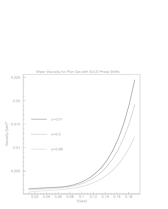
Figure 5: Shear viscosity of the pion gas from the $SU(3)$ Inverse Amplitude Method phase shifts.

Next we turn to some more realistic pion interactions. These are provided by the simple analytical fit to the pion phase shifts from (60) and by the $SU(2)$ or $SU(3)$ inverse amplitude method. The results are quite consistent and plotted in figures 3, 4 and 5 respectively. The difference between them gives us an idea of the sensitivity of the viscosity to the employed phase shifts, since all sets of phase shifts are reasonable. To what precision these scattering phase shifts are known is an ongoing debate warriors and if a future determination pinned them down with greater accuracy a much better prediction for the viscosity could be made, since the parameterization used for the phase shifts seems to be one of the largest uncertainty sources in the present (already realistic) computation.

VIII Full Pion, Kaon, Eta Gas Viscosity.

Figure 6: Separate effect of adding $K$ or $\eta$ mesons to the pion gas, with their chemical potential vanishing. The kaons are by far more important (partly due to their multiplicity).

Finally we turn to a gas including kaon and eta mesons. We first introduce either type of particle separately and plot it in fig. 6. The effect of kaons is much more dramatic than the effect of eta mesons. By comparing with fig. 5 which was calculated with the same pion phase shifts we can see that already at 100 MeV the addition of the kaons alone give a viscosity way bigger than present in the pion gas. The sensitivity of this calculation on the pion fugacity (density) is also very large. The combined effect of adding both kaons and etas to the gas is finally plotted in fig. 7. Of course, in a relativistic heavy ion collision we expect the chemical freeze-out of heavier mesons to occur before and therefore we need to introduce chemical potentials for all species, those corresponding to the heavier mesons being larger than for lighter mesons.

Figure 7: The shear viscosity for the full meson ($\pi$, K, $\eta$) gas in linear (upper) and semilogarithmic (lower) panels. At very low $z$ and $T$ the reader can appreciate how the non-relativistic behaviour ($\eta\propto\sqrt{T}$) is recovered. The chemical potential for both $K$ and $\eta$ has been set to zero.

In natural units the viscosity has dimensions of an energy cubed, and indeed at moderate to high temperatures, the viscosity approximately follows a power law with an exponent near (and slightly above) 3, which is suggesting the viscosity is dominated by the highest energy pions where the mass and chemical potential scales are less important than the momentum scale. The low temperature behaviour of the viscosity is plotted in figure 8 where we observe how at low temperature the effect of adding the more massive particles is to decrease the plateau in which the viscosity is approximately independent of the temperature.

Figure 8: The shear viscosity for the full meson ($\pi$, K, $\eta$) gas at lower temperature. The chemical potentials are $\mu_{\pi}=100$ MeV, $\mu_{K}=250$ MeV, $\mu_{\eta}=300$ MeV. The low energy plateau is reduced by adding more species, as kaons and etas behave less as Goldstone bosons than the pion, so their low energy interactions are already larger and don’t see such a large relative increase as the pion’s with collision energy, and the viscosity increases more rapidly with the temperature as the number of species is increased.

The resulting viscosities for various temperatures and chemical potentials are tabulated in table 3 and convey our final results.

Table 3: Shear viscosity at various values of chemical potentials and temperature. Units are MeV ($T$ and $\mu_{a}$) and $(100\ {\rm MeV})^{3}$ ($\eta_{s}$). The error due to the Montecarlo evaluation of the 5-D integral is (5) on the last significant digit of the viscosity. This calculation employs the Inverse Amplitude Method phase shifts within $SU(3)$.

$T$	$\mu_{\pi}$	$\mu_{K}$	$\mu_{\eta}$	$\eta_{s}$
100	0	0	0	3.37
100	0	100	150	5.24
100	0	200	250	9.96
100	100	100	150	3.04
100	100	200	250	4.56
100	100	400	450	19.0
125	0	0	0	7.13
125	0	100	150	11.4
125	0	200	250	20.1
125	100	100	150	6.31
125	100	200	250	9.69
125	100	400	450	31.6
150	0	0	0	15.4
150	0	100	150	24.2
150	0	200	250	39.6
150	100	100	150	13.4
150	100	200	250	20.2
150	100	400	450	53.8

IX Comparison with Other Approaches and Discussion

The viscosity of a pion gas has already been treated by D. Davesne in davesne as a quantum relativistic system. In this pioneering work to solve the relativistic Uehling-Uhlenbeck equation the pion interaction was modelled following ref. prakash3 , which corresponds to the phase shifts (60) above. If we consider only a pion gas and employ the same set of phase shifts then we can approximately reproduce this results. Furthermore, we document the sensitivity of the viscosity to the parameterization of the phase shifts, which was not treated in this reference. We have also streamlined the numerical solution of the transport equation, by employing a new family of orthogonal polynomials which allows to systematically extract better approximations if so wished, and performing a Montecarlo evaluation of the collision multidimensional integral, whereas the more analytical treatment in davesne is also somewhat more obscure. It is also interesting that a relaxation time estimation of the Boltzmann equation (with no quantum corrections) permits to approximate the shear viscosity of a pion/kaon gas in prakash4 ; prakash1 . The order of magnitude and qualitative behaviour as a function of temperature are correct. We obtain somewhat larger results which are not unexpected as quantum corrections in a Bose gas may tend to decrease the cross section for scattering to initially unpopulated states, increasing the viscosity, and furthermore some difference is expected due to our use of the $SU(3)$ phase shifts.

To summarize, we have presented a systematic calculation of the shear viscosity in meson matter at moderate temperatures. We have found the viscosity to behave as expected from a non-relativistic gas point of view at very low temperatures, to stabilize and even decrease (depending on the chemical potential) at small temperatures because of the larger cross section at increasing energies (the decrease would be a typical effect of a Goldstone boson gas) and to follow a positive power law at moderate to high temperatures. At high $T$ (above 150 MeV) our approach should be less reliable because we are employing scattering phase shifts parameterized up to momenta of 1 GeV and with sizeable temperatures, states with higher momentum start being populated. Eventually one reaches the phase transition temperature, and any results obtained from within the chirally broken phase (as built-in in our use of meson fields and chiral perturbation theory) is simply not appropriate. Extensions of this work to include nucleons or to evaluate other interesting transport coefficients are now straight-forward.

Appendix A Linearized Transport Equation Coefficients

In this appendix we provide the matrix elements necessary for the first order Chapman-Enskog solution of the transport equation. The right-hand side of the system (47) is

$$\left(\begin{array}[]{c}C_{\pi}\\ C_{K}\\ C_{\eta}\end{array}\right)=\left(\begin{array}[]{c}\frac{4\pi m_{\pi}^{6}}{3\xi_{\pi}}l_{5/2}(y_{\pi},z_{\pi})\\ \frac{4\pi m_{K}^{6}}{3\xi_{K}}l_{5/2}(y_{K},z_{K})\\ \frac{4\pi m_{\eta}^{6}}{3\xi_{\eta}}l_{5/2}(y_{\eta},z_{\eta})\end{array}\right)\ .$$ (66)

The left-hand side matrix elements can be given by the formula

(67)

$$A_{ab}=\frac{\xi_{a}\xi_{b}}{z_{a}z_{b}}\int d\sigma_{ab}v_{\rm rel}d\vec{p}d\vec{p}_{1}e^{\beta(E-m_{a}-m_{b})}f_{0a}f_{0b1}f_{0a}^{\prime}f_{0b1}^{\prime}$$

$$\left(1-z_{a}e^{\beta(E(p)-m_{a})}\right)(\delta_{ik}\delta_{jl})-\frac{1}{3}\delta_{ij}\delta_{kl})p_{i}p_{j}({\bf A}_{ab})_{kl}$$

in terms of a tensor $({\bf A}_{ab})_{kl}$ which takes the values

$$({\bf A^{\pi}}_{11})_{kl}=p^{{}^{\prime}k}p^{{}^{\prime}l}(1-e^{-\beta(E^{\prime}-\mu_{\pi})})-p^{k}p^{l}(1-e^{-\beta(E(p)-\mu_{\pi})})$$

$$+p_{1}^{{}^{\prime}k}p_{1}^{{}^{\prime}l}(1-e^{-\beta(E_{1}^{\prime}-\mu_{\pi})})-p_{1}^{k}p_{1}^{l}(1-e^{-\beta(E_{1}-\mu_{\pi})})$$

$$({\bf A^{K}}_{11})_{kl}=({\bf A^{\eta}}_{11})_{kl}=$$

$$p^{{}^{\prime}k}p^{{}^{\prime}l}(1-e^{-\beta(E^{\prime}-\mu_{\pi})})-p^{k}p^{l}(1-e^{-\beta(E(p)-\mu_{\pi})})$$

$$({\bf A}_{12})_{kl}=p_{1}^{{}^{\prime}k}p_{1}^{{}^{\prime}l}(1-e^{-\beta(E_{1}^{\prime}-\mu_{K})})-p_{1}^{k}p_{1}^{l}(1-e^{-\beta(E_{1}-\mu_{K})})$$

$$({\bf A}_{13})_{kl}=p_{1}^{{}^{\prime}k}p_{1}^{{}^{\prime}l}(1-e^{-\beta(E_{1}^{\prime}-\mu_{\eta})})-p_{1}^{k}p_{1}^{l}(1-e^{-\beta(E_{1}-\mu_{\eta})})$$

$$({\bf A}_{22})_{kl}=p^{{}^{\prime}k}p^{{}^{\prime}l}(1-e^{-\beta(E^{\prime}-\mu_{K})})-p^{k}p^{l}(1-e^{-\beta(E(p)-\mu_{K})})$$

$$({\bf A}_{21})_{kl}=({\bf A}_{31})_{kl}=$$

$$p_{1}^{{}^{\prime}k}p_{1}^{{}^{\prime}l}(1-e^{-\beta(E_{1}^{\prime}-\mu_{\pi})})-p_{1}^{k}p_{1}^{l}(1-e^{-\beta(E_{1}-\mu_{\pi})})$$

$$({\bf A}_{33})_{kl}=p^{{}^{\prime}k}p^{{}^{\prime}l}(1-e^{-\beta(E^{\prime}-\mu_{\eta})})-p^{k}p^{l}(1-e^{-\beta(E(p)-\mu_{\eta})})$$

Appendix B Orthogonal polynomials.

In solving the Uehling-Uhlenbeck equation with relativistic kinematics and quantum statistics, one needs to integrate over the measure

$$d\mu_{r}(x;y,z)=w_{r}(x;y,z)dx=$$ (68)

$$\frac{x^{r}dx}{\sqrt{1+x}\left(z^{-1}e^{y(\sqrt{1+x}-1)}-1\right)}$$

With the variable $x$ and parameters $y,z$ defined in (14) above, with ranges $z\in(0,1)$, $y\in(0,\infty)$, $x\in(0,\infty)$. The index $r\geq 1$ takes in typical applications a half-integer value due to relativistic kinematics. It can be easily seen that $d\mu^{r}$ is a valid measure, positive definite, with bound integrals

$$\mu_{n}=\int_{0}^{\infty}dxW_{r}(x;y,z)x^{n}<\infty$$

for $n$ a positive integer. As a consequence we can define a family of orthogonal polynomials analogous to the Sonine polynomials, but more appropriate for a relativistic Bose-Einstein gas, which can conveniently be chosen monic (coefficient of highest dimension term equals one), denoted $P^{s}(x;,y,z)$ and with an orthogonalization

$$\int_{0}^{\infty}dxW_{r}(x;y,z)P^{s}_{r}(x;,y,z)P^{t}_{r}(x;,y,z)=\delta^{st}A^{s}_{r}(y,z)\ .$$ (69)

Since the polynomials are considered monic, $A$ is not unity. In the calculation presented we have considered a meson gas slightly out of equilibrium, where a good approximation is achieved by keeping only the first polynomial in the expansion of $g(p)$ defined in (30) above. This has been verified in silvia in the non-relativistic limit. Therefore in this calculation we only need to evaluate the $A_{00}(y,z)$ function.