Exploring Leptonic CP Violation by Reactor and Neutrino Superbeam Experiments

Abstract

We point out the possibility that reactor measurement of $\theta_{13}$, when combined with high-statistics $\nu_{e}$ appearance accelerator experiments, can detect leptonic CP violation. Our proposal is based on a careful statistical analysis under reasonable assumptions on systematic errors, assuming 2 years running of the neutrino mode J-PARC $\rightarrow$ Hyper-Kamiokande experiment and a few years running of a reactor experiment with 100ton detectors at the Kashiwazaki-Kariwa nuclear power plant. We show that the method can be arranged to be insensitive to the intrinsic parameter degeneracy but is affected by the one due to unknown sign of $\Delta m^{2}_{31}$.

I Introduction

After the pioneering and the long-term extensive efforts in the atmospheric SKatm , the solar solar , the accelerator K2K , and the reactor KamLAND experiments, we have grasped the structure of lepton flavor mixing in the (2-3) and the (1-2) sectors of the Maki-Nakagawa-Sakata (MNS) matrix MNS . Now we are left with the unique unknown (1-3) sector of the MNS matrix, in which there live the third mixing angle $\theta_{13}$, which is known to be small CHOOZ , and the completely unknown CP-violating leptonic Kobayashi-Maskawa phase $\delta$ KM .

Detecting leptonic CP violation is one of the most challenging goals in particle physics. A popular method for measuring the CP-violating phase is by long-baseline (LBL) accelerator neutrino experiments using either conventional neutrino superbeam J-PARC ; SPL ; BNL , or an intense beam from muon storage ring nufact . If $\theta_{13}$ is not too small, it is likely that leptonic CP violation is first explored by LBL experiments with conventional superbeam superbeam .

To measure CP-violating phase the LBL experiments must run not only with the neutrino mode but also with the antineutrino mode. Apart from the problem of parameter degeneracy Burguet-C ; MNjhep01 ; KMN02 ; octant ; BMW1 ; MNP2 , these measurement would allow us to determine the CP-violating phase $\delta$ to a certain accuracy. In the Japan Proton Accelerator Research Complex (J-PARC) $\rightarrow$ Hyper-Kamiokande project with upgraded 4MW beam of 50GeV accelerator at J-PARC, the accuracy of determination of $\delta$ is expected to be $\simeq$ 20 degrees at 3$\sigma$ CL J-PARC .

Running the experiment with antineutrino mode, however, is possible only by overcoming a variety of difficulties, much greater ones compared with those in neutrino mode operation. Even if we ignore the issue of slightly less intense $\pi^{-}$ beam compared to $\pi^{+}$ beam, the antineutrino cross sections are smaller by factor of $\simeq$ 3 than neutrino cross sections, which results in three-times longer period of data taking, 6 years of $\bar{\nu}$-mode compared to 2 years of $\nu$-mode operation in the J-PARC $\rightarrow$ Hyper-Kamiokande (hereafter abbreviated as JPARC-HK) experiment. Moreover, the background in $\bar{\nu}_{e}$ appearance detection, according to the current estimate, are larger by factor of $\simeq$ 2 compared with those in $\nu_{e}$ detection. Hence, antineutrino-mode measurement may be better characterized as an independent experiment rather than the in-situ measurement. Considering three times longer running time it is certainly worthwhile to think about an alternative which can run simultaneously with neutrino-mode superbeam appearance experiments.

In this paper, we point out that a reactor experiment can serve for such purpose. We demonstrate that reactor experiments for measuring $\theta_{13}$ with reasonable assumptions on their systematic errors can uncover the leptonic CP violation when combined with high-statistics neutrino-mode superbeam experiments. In fact, we have pointed out such possibility in our previous communication MSYIS , in which we have demonstrated the complementary role of the reactor and the LBL accelerator experiments in determination of the remaining neutrino mixing parameters. The treatment in this paper quantifies our proposal and thereby complements and further strengthen our viewpoint of the LBL-reactor complementarity. A quantitative treatment of sensitivity for detecting CP violation by reactor-LBL combination was also attempted in Ref. Munich but with no indication of signal. See Ref. krasnoyarsk ; kashkari ; diablo for detailed description of possible experimental designs for reactor experiments for measuring $\theta_{13}$.

We remark that the sensitivity to CP violation by our reactor-LBL combined method suffers from the problem of parameter degeneracy. However, it can be arranged so that it is insensitive to the intrinsic parameter degeneracy Burguet-C . If the superbeam experiment is done at the oscillation maximum the combined measurement will allow us to determine $\sin{\delta}$. Obviously, the measurement by itself cannot resolve the ambiguity $\delta\leftrightarrow\pi-\delta$, but it does not produce a fake CP violation. We have to note that our method suffers from the problem of degeneracy due to unknown sign of $\Delta m^{2}_{31}$ MNjhep01 . Even in the case of the JPARC-HK experiment in which the matter effect is only modest, it does affects the CP sensitivity because the degenerate solutions of $\delta$ differ by $\sim\pi/2$ in overlapping region of two ellipses in the bi-probability plot MNjhep01 . Therefore, it is important to know the sign of $\Delta m^{2}_{31}$ prior to the reactor-LBL measurement of $\delta$. While the octant ambiguity of $\theta_{23}$ octant may also affect the CP sensitivity, we do not try to elaborate this point in the present paper. See, however, (1) in the concluding remarks.

We emphasize that reactor experiment cannot replace the antineutrino-mode superbeam experiments. It is because the reactor-LBL combined method can detect leptonic CP violation only up to $\simeq$ 2$\sigma$ CL. Nevertheless, we believe that such reactor-LBL combined measurement has a great merit. It will give us the first grip of the structure of leptonic CP violation. It will also merit the then ongoing neutrino-mode and the following antineutrino-mode superbeam experiments themselves; Even a rough knowledge of the feature of CP violation would be very helpful to optimize the setting (such as relative time sharing of $\nu$ and $\bar{\nu}$ modes) of the difficult and extremely long-term experiment.

II Reactor-LBL Combined Measurement of CP Violation

The principle of detection of leptonic CP violation in a reactor-LBL combined measurement is very simple. First let us remind the readers the characteristic features of reactor measurement of $\theta_{13}$. As we have discussed in length in Ref. MSYIS , reactor experiment can serve for pure measurement of $\theta_{13}$ assuming that $\Delta m^{2}_{31}$ is accurately determined by disappearance measurement of $P(\nu_{\mu}\rightarrow\nu_{\mu})$ in LBL experiments. Namely, it is not contaminated by uncertainties due to unknown CP phase $\delta$, the matter effect, and possibly to the octant ambiguity $\theta_{23}\rightarrow\pi/2-\theta_{23}$ from which $\nu_{e}$ appearance measurement by LBL experiment suffers.

Now LBL $\nu_{e}$ appearance experiment will observe the neutrino oscillation probability $P(\nu_{\mu}\rightarrow\nu_{e})$. In leading order in $\Delta m^{2}_{21}/\Delta m^{2}_{31}$ it takes the form golden

$$P(\nu_{\mu}\rightarrow\nu_{e})\equiv P(\nu)_{\pm}=X_{\pm}s_{13}^{2}+Y_{\pm}s_{13}\cos{\left(\delta\pm\frac{\Delta_{31}}{2}\right)}+P_{\odot},$$ (1)

where $\pm$ refers to the sign of $\Delta m^{2}_{31}$. The coefficients $X_{\pm}$, $Y_{\pm}$, and $P_{\odot}$ are given by

$$X_{\pm} = 4s^{2}_{23}\left(\frac{\Delta_{31}}{B_{\mp}}\right)^{2}\sin^{2}{\left(\frac{B_{\mp}}{2}\right)},$$ (2)

$$Y_{\pm} = \pm 8c_{12}s_{12}c_{23}s_{23}\left(\frac{\Delta_{21}}{aL}\right)\left(\frac{\Delta_{31}}{B_{\mp}}\right)\sin{\left(\frac{aL}{2}\right)}\sin{\left(\frac{B_{\mp}}{2}\right)},$$ (3)

$$P_{\odot} = c^{2}_{23}\sin^{2}{2\theta_{12}}\left(\frac{\Delta_{21}}{aL}\right)^{2}\sin^{2}{\left(\frac{aL}{2}\right)}$$ (4)

with

$$\Delta_{ij}\equiv\frac{|\Delta m^{2}_{ij}|L}{2E}\quad{\rm and}\quad B_{\pm}\equiv\Delta_{31}\pm aL,$$ (5)

where $a=\sqrt{2}G_{F}N_{e}$ denotes the index of refraction in matter with $G_{F}$ being the Fermi constant and $N_{e}$ a constant electron number density in the earth. We use in this paper the standard notation of the MNS matrix PDG . The mass squared difference of neutrinos is defined as $\Delta m^{2}_{ji}\equiv m^{2}_{j}-m^{2}_{i}$ where $m_{i}$ is the mass of the $i$-th eigenstate.

There exist number of reasons for tuning the beam energy to the oscillation maximum $\Delta_{13}=\pi$ in doing the appearance and the disappearance measurement in LBL experiments, as listed in KMN02 . In this case, $\cos{\left(\delta\pm\frac{\Delta_{13}}{2}\right)}=\mp\sin{\delta}$ and (1) can be solved for $\sin{\delta}$ as

$$\sin{\delta}=\frac{P(\nu)-P_{\odot}-X_{\pm}s_{13}^{2}}{\mp Y_{\pm}s_{13}}.$$ (6)

We note that, since $\theta_{13}$ can be measured by reactor experiments, the right-hand side (RHS) of (6) consists solely of experimentally measurable quantities. Therefore, LBL measurement of $P(\nu_{\mu}\rightarrow\nu_{e})$, when combined with the reactor experiment, implies measurement of $\sin{\delta}$.

In the rest of this paper, we try to elaborate our treatment by including suitably estimated experimental uncertainties of both LBL and the reactor experiments. As indicated in (6), the accuracy of measurement of $\sin{\delta}$ solely depends upon how precisely $P(\nu)$ and $s_{13}$ in the RHS can be determined in LBL and reactor experiments, respectively. We take the best possible case among the concrete proposals of LBL experiments currently available in the community, the JPARC-HK experiment assuming 4MW beam power and 540 kton as the fiducial volume of the detector Hyper-K . However, most probably our conclusion does not heavily depend on any detailed experimental setting in the particular experiment, once the accuracy of measurement of the $\nu_{e}$ appearance probability reaches to that level and if the baseline is not too long. For the reactor experiment, we present our results in units of $\text{GW}_{\text{th}}\cdot\mbox{ton}\cdot\mbox{year}$ exposure to allow application to wider class of experiments. Our results may be useful to indicate what condition must be met to uncover the leptonic CP violation in such reactor-LBL combined measurement.

III Treatment of errors in LBL and reactor experiments

To carry out quantitative analyses of the sensitivity for detecting CP violation, we must first establish the method for statistical treatment of LBL and reactor experiments.

III.1 Treatment of errors in the JPARC-HK experiment

We consider neutrino-mode appearance measurement for 2 years in the JPARC-HK experiment. For definiteness, we use the neutrino flux estimated for the off-axis $2^{\circ}$ beam J-PARC . We define $\Delta\chi^{2}$ for the experiment as

$$\Delta\chi^{2}_{{\text{J-PARC}}\nu}\equiv\frac{\left(N_{\nu}-N_{\nu}^{\text{best}}\right)^{2}}{N_{\nu}^{\text{best}}+N_{\text{BG}}+\sigma_{\text{S}}^{2}(N_{\nu}^{\text{best}})^{2}+\sigma_{\text{BG}}^{2}(N_{\text{BG}})^{2}},$$ (7)

where $N_{\nu}$ and $N_{\text{BG}}$ represent the expected number of signal and background events, respectively, computed with the cross section in kameda . $N_{\nu}^{\text{best}}$ is defined as the number of signal event $N_{\nu}$ calculated with the best-fit values of the “experimental data”, which is to be tested against the CP conserving hypothesis, $\delta=0$. $\sigma_{\text{S}}$ and $\sigma_{\text{BG}}$ represent the fractional uncertainties of the estimation of the number of signal and background events, respectively. Following J-PARC , we use $\sigma_{\text{S}}=\sigma_{\text{BG}}=2\%$ in our analysis. (See Sect. IV for more about how to use $\Delta\chi^{2}$ in our procedure to determine the sensitivity region for CP violation.)

While we do not use the spectrum information in a direct way in our analysis, we need to estimate how the experimental event selection affects the spectrum to calculate the number of signal and background events. The most important cut is to suppress the background events due to $\pi^{0}$. We use the simulated spectra after the cut calculated by the JPARC-SK group kobayashi and evaluate the reduction rate due to cut in each energy bin of 50MeV width. The procedure is applied to calculate the number of signal after the cut for any values of mixing parameters. In this way, the total numbers of events within energy range 0.4-1.2GeV are calculated and used in our analysis.

III.2 Treatment of errors in the reactor experiment

In this paper we consider the case of single reactor and two (near and far) detector complex. The far detector is placed 1.7km away from the reactor, the optimal distance for $|\Delta m^{2}_{31}|=2.5\times 10^{-3}\,{\text{eV}}^{2}$. We assume that a near detector identical with the far detector is placed 300m away from the reactor to reduce systematic errors.

We consider four types of systematic errors: $\sigma_{\text{DB}}$, $\sigma_{\text{Db}}$, $\sigma_{\text{dB}}$, and $\sigma_{\text{db}}$. The subscript D (d) represents the fact that the error is correlated (uncorrelated) between detectors. The subscript B (b) represents that the error is correlated (uncorrelated) among bins. To indicate nature of these respective errors, we list below some examples of the errors in each category:

$\sigma_{\text{DB}}$: error in estimation of reactor power

$\sigma_{\text{Db}}$: error in estimation of detection cross sections

$\sigma_{\text{dB}}$: error in estimation of fiducial volume of each detector

$\sigma_{\text{db}}$: errors inherent to detectors such as artificial firing of photomultiplier tubes

Although the values of $\sigma_{\text{dB}}$ for far and near detectors, for example, can be different from each other, we neglect such difference for simplicity. The values of systematic errors we assume are listed in Table 1.

		between detectors
		correlated	uncorrelated	single detector
between bins	correlated	$\sigma_{\text{DB}}=2.5\%$	$\sigma_{\text{dB}}=0.5\%$	$\sigma_{\text{B}}\simeq 2.6\%$
	uncorrelated	$\sigma_{\text{Db}}=2.5\%$	$\sigma_{\text{db}}=0.5\%$	$\sigma_{\text{b}}\simeq 2.6\%$
total number of events		$\sigma_{\text{D}}\simeq 2.6\%$	$\sigma_{\text{d}}\simeq 0.5\%$	$\sigma_{\text{sys}}\simeq 2.7\%$

Table 1: Listed are assumed values of systematic errors $\sigma_{\text{DB}}$, $\sigma_{\text{Db}}$, $\sigma_{\text{dB}}$, and $\sigma_{\text{db}}$. The subscripts D (d) and B (b) are represent the correlated (uncorrelated) error among detectors and bins, respectively. Using those four values, the errors for the total number of events and for single detector are calculated.

As will be briefly explained in the appendix, the errors $\sigma_{\text{D}}$ and $\sigma_{\text{d}}$ for the total number of events are obtained as

$$\sigma_{\text{D}}^{2}=\sigma_{\text{DB}}^{2}+\sigma_{\text{Db}}^{2}\frac{\sum_{i}(N_{ai}^{\text{best}})^{2}}{\left(\sum_{i}N_{ai}^{\text{best}}\right)^{2}},\ \ \sigma_{\text{d}}^{2}=\sigma_{\text{dB}}^{2}+\sigma_{\text{db}}^{2}\frac{\sum_{i}(N_{ai}^{\text{best}})^{2}}{\left(\sum_{i}N_{ai}^{\text{best}}\right)^{2}},$$ (8)

where $a=n,f$ are the index for near and far detectors, and $i$ runs over number of bins. We use 14 bins of $0.5{\text{MeV}}$ width in 1-8MeV window of visible energy, $E_{\text{visi}}=E_{\bar{\nu}_{e}}-0.8{\text{MeV}}$. The coefficient of $\sigma_{\text{Db}}^{2}$ and $\sigma_{\text{db}}^{2}$ is about 1/9 in our analysis almost independently of $a$. Since relative normalization errors are $\sqrt{2}$ times of uncorrelated errors, $\sigma_{\text{d}}\simeq 0.5\%$ is consistent with the value used in MSYIS . In Ref. MSYIS , the most pessimistic assumption $\sigma_{\text{DB}}=\sigma_{\text{dB}}=0$ was taken for bin-by-bin distribution of errors. The value of $\sigma_{\text{sys}}^{2}\equiv\sigma_{\text{D}}^{2}+\sigma_{\text{d}}^{2}$ is also consistent with the total systematic error of the CHOOZ experiment. In summary, we feel that the errors listed in Table 1 are not too optimistic ones and are likely to be realized in the setting discussed in krasnoyarsk ; kashkari ; diablo .

Our definition of $\Delta\chi^{2}_{\text{react}}$ is

$$\Delta\chi^{2}_{\text{react}} \equiv \min_{\text{$\alpha$'s}}\sum_{a=f,n}\left[\sum_{i=1}^{14}\left\{\frac{\left(N_{ai}-(1+\alpha_{i}+\alpha_{a}+\alpha)N^{\text{best}}_{ai}\right)^{2}}{N^{\text{best}}_{ai}+\sigma_{\text{db}}^{2}(N^{\text{best}}_{ai})^{2}}+\frac{\alpha_{i}^{2}}{\sigma_{\text{Db}}^{2}}\right\}+\frac{\alpha_{a}^{2}}{\sigma_{\text{dB}}^{2}}\right]+\frac{\alpha^{2}}{\sigma_{\text{DB}}^{2}},$$ (9)

where $N_{ai}$ represents the theoretical number of events at $a$-detector within $i$-th bin. Again, $N_{ai}^{\text{best}}$ is defined as the number of signal event calculated with the best-fit parameters of the “experimental data”. The minimization in (9) is achieved analytically, and then we obtain

$$\Delta\chi^{2}_{\text{react}}=(\vec{x}^{\text{T}},\vec{y}^{\text{T}})V^{-1}\left(\begin{array}[]{c}\vec{x}\\ \vec{y}\\ \end{array}\right),$$ (12)

$$\vec{x}^{\text{T}}\equiv\left(\frac{N_{f1}-N^{\text{best}}_{f1}}{N^{\text{best}}_{f1}},\cdots\right),\ \vec{y}^{\text{T}}\equiv\left(\frac{N_{n1}-N^{\text{best}}_{n1}}{N^{\text{best}}_{n1}},\cdots\right),$$ (13)

$$V\equiv\text{diag}\left(\frac{1}{N^{\text{best}}_{f1}},\cdots,\frac{1}{N^{\text{best}}_{n1}},\cdots\right)$$

$$\hskip 56.9055pt{}+\sigma_{\text{db}}^{2}I_{28}+\sigma_{\text{dB}}^{2}\left(\begin{array}[]{cc}H_{14}&0\\ 0&H_{14}\end{array}\right)+\sigma_{\text{Db}}^{2}\left(\begin{array}[]{cc}I_{14}&I_{14}\\ I_{14}&I_{14}\end{array}\right)+\sigma_{\text{DB}}^{2}H_{28},$$ (18)

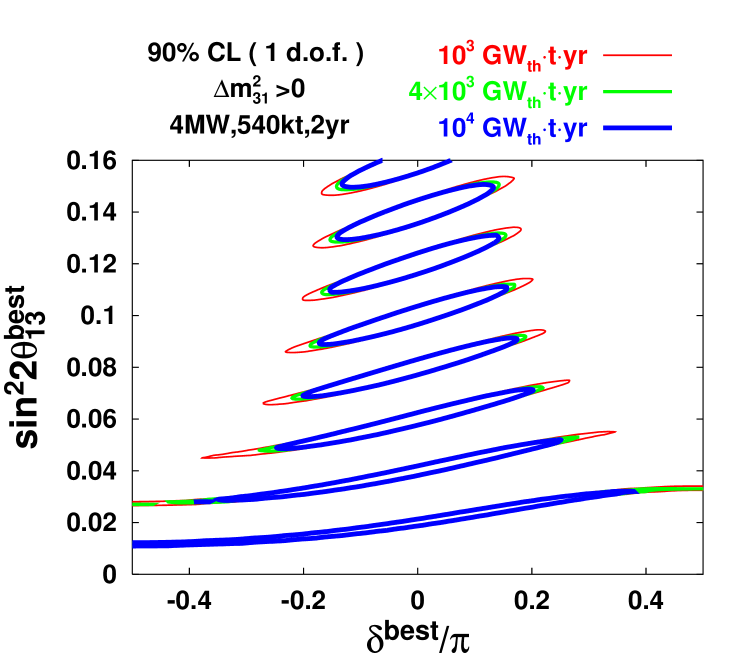
Figure 2: The contours are plotted for eight assumed values of $\sin^{2}{2\theta_{13}}$ which range from 0.02 to 0.16 to indicate the regions consistent with the hypothesis $\delta=0$ at 90% CL ($\Delta\chi^{2}_{\text{CP}}=2.7$) by the reactor-LBL combined measurement. If an experimental best fit point falls into outside the envelope of those regions, it gives an evidence for leptonic CP violation at 90% CL. The thin-solid (red), solid (green), and thick-solid (blue) lines are for $10^{3}$, $4\times 10^{3}$, and $10^{4}\text{GW}_{\text{th}}\cdot\mbox{ton}\cdot\mbox{year}$ exposure of a reactor experiment, respectively, corresponding to about 0.5, 2, and 5 years exposure of 100 ton detectors at the Kashiwazaki-Kariwa nuclear power plant. For the JPARC-HK experiment, 2 years measurement with off-axis $2^{\circ}$ $\nu_{\mu}$ beam is assumed. (See the text for more details.) The normal mass hierarchy, $\Delta m^{2}_{31}>0$, is assumed.

where $I_{n}$ represents the $n\times n$ identity matrix and $H_{n}$ represents the $n\times n$ matrix whose elements are all unity. Notice that an infinitely good sensitivity is obtained for infinite number of events if $\sigma_{\text{db}}$ vanishes because $\det(V)$ goes to zero for the case which explains the apparently curious behavior seen in Fig. 2 of Munich . See stump for more about the equivalence between the “pull” and the covariance matrix methods.

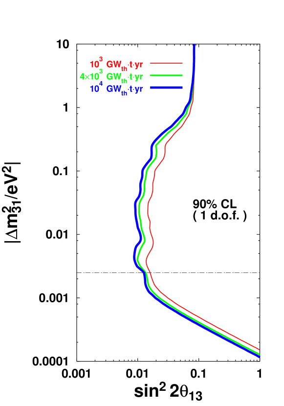
Figure 1: The excluded regions at 90% CL in the absence of $\bar{\nu}_{e}$ disappearance ($\theta_{13}^{\text{best}}=0$) are drawn for $10^{3}$, $4\times 10^{3}$, and $10^{4}$ $\text{GW}_{\text{th}}\cdot\mbox{ton}\cdot\mbox{year}$ exposure of a reactor experiment by thin-solid (red), solid (green), and thick-solid (blue) lines, respectively. The far (near) detector is placed 1.7km (300m) away from the reactor. We assume that $|\Delta m^{2}_{31}|$ is precisely measured by LBL experiments and adopt the analysis with one degree of freedom ($\Delta\chi^{2}_{\text{react}}=2.7$). We use the value $|\Delta m^{2}_{31}|=2.5\times 10^{-3}{\text{eV}}^{2}$ as indicated by the dashed-doted line in the figure. In our analysis, we use 14 bins of 0.5MeV width in 1-8MeV window of visible energy with the systematic errors listed in Table 1.

To indicate the expected sensitivity of the reactor experiment with the systematic errors listed in Table 1, we present in Fig. 1 the excluded region in $\sin^{2}{2\theta_{13}}$-$|\Delta m^{2}_{31}|$ space in the absence of flux depletion ($\theta_{13}^{\text{best}}=0$) for $10^{3}$, $4\times 10^{3}$, and $10^{4}$ $\text{GW}_{\text{th}}\cdot\mbox{ton}\cdot\mbox{year}$ exposure. The $\bar{\nu}_{e}$ detection efficiency of 70% is assumed CHOOZ ; MSYIS . The number of events expected during these exposure are about $10^{5}$, $4\times 10^{5}$, $10^{6}$ $\bar{\nu}_{e}$ events, respectively, at the far detector. Notice that what we mean by numbers in units of $\text{GW}_{\text{th}}$ is the thermal power actually generated from reactors and it should not be confused with the maximal thermal power of reactors. Assuming average 80% operation efficiency the above three cases correspond approximately to 0.5, 2, and 5 years running, respectively, for 100 ton detector at the Kashiwazaki-Kariwa nuclear power plant whose maximal thermal power is $24.3\text{GW}_{\text{th}}$.

IV Estimation of Sensitivity of Reactor-LBL Combined Detection of CP Violation

To estimate the sensitivity of the reactor-LBL combined measurement to leptonic CP violation, we define the combined $\Delta\chi^{2}$ as

$$\Delta\chi^{2}_{\text{CP1}}(\delta;\delta^{\text{best}},\sin^{2}{2\theta_{13}^{\text{best}}}) \equiv \min_{\sin^{2}{2\theta_{13}}}\Delta\chi^{2}_{\text{CP}}(\delta,\sin^{2}{2\theta_{13}};\delta^{\text{best}},\sin^{2}{2\theta_{13}^{\text{best}}})$$ (19)

$$\equiv \min_{\sin^{2}{2\theta_{13}}}\Bigl{\{}\Delta\chi^{2}_{{\text{J-PARC}}\nu}(\delta,\sin^{2}{2\theta_{13}};\delta^{\text{best}},\sin^{2}{2\theta_{13}^{\text{best}}})$$

$$\hskip 99.58464pt{}+\Delta\chi^{2}_{\text{react}}(\sin^{2}{2\theta_{13}};\sin^{2}{2\theta_{13}^{\text{best}}})\Bigr{\}}.$$

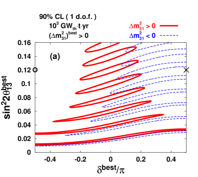
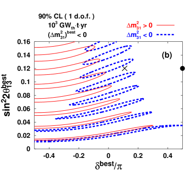
Figure 3: The contours which surround the region consistent with CP conservation are plotted in Fig. 3a (3b) by assuming $(\Delta m^{2}_{31})^{\text{best}}>0$ ($(\Delta m^{2}_{31})^{\text{best}}<0$) as nature’s choice. If the right (wrong) sign is used as the hypothesis with $\delta=0$, the contours indicated by the thick (thin) lines result in both figures. The three symbols, a cross, open and solid circles are placed on the figures as well as in Fig. 4 to indicate the relationship between observed numbers of events and the results of CP sensitivity analysis.

We take the following procedure in our analysis. We pick up a point in the two-dimensional parameter space spanned by $\delta^{\text{best}}$ and $\sin^{2}{2\theta_{13}^{\text{best}}}$ and make the hypothesis test on whether the point is consistent with CP conservation within 90% CL. For this purpose, we use the projected $\Delta\chi^{2}$ onto one-dimensional $\delta$ space, $\Delta\chi^{2}_{\text{CP1}}$, as defined in (19) and then the statistical criterion for 90% CL is $\Delta\chi^{2}_{\text{CP1}}\leq 2.7$. Then, a collection of points in the parameter space which are consistent with CP conservation form a region surrounded by a contour in $\delta^{\text{best}}$-$\sin^{2}{2\theta_{13}^{\text{best}}}$ space, as will be shown in Figs. 2-3 below.

The neutrino mixing parameters are taken as follows: $|\Delta m_{31}^{2}|=2.5\times 10^{-3}{\text{eV}}^{2}$, $\Delta m_{21}^{2}=7.3\times 10^{-5}{\text{eV}}^{2}$, $\tan^{2}{\theta_{12}}=0.38$, and $\sin^{2}{2\theta_{23}}=1$. Notice that the high-$\Delta m^{2}_{21}$ LMA-II solar neutrino solution is now excluded at 3$\sigma$ CL by the global analysis of all data with reanalyzed day-night variation of flux at Super-Kamiokande SK_daynight , and at 99% CL by the one with SNO salt phase data SNO_salt . The earth matter density is taken to be $\rho=2.3\,\mbox{g}\cdot\mbox{cm}^{-3}$ koike-sato and the electron number density is computed with electron fraction $Y_{e}=0.5$.

IV.1 CP sensitivity in the case of known sign of $\Delta m^{2}_{31}$

In Fig. 2, the regions consistent with CP conservation at 90% CL are drawn for $\Delta m^{2}_{31}>0$ case in the region $-\pi/2\leq\delta^{\text{best}}\leq\pi/2$. The thin-solid, the solid, and the thick-solid lines are for $10^{3}$, $4\times 10^{3}$, and $10^{4}\text{GW}_{\text{th}}\cdot\mbox{ton}\cdot\mbox{years}$, respectively, and the regions consistent with CP conservation are within the envelope of these contours. We remark that the present constraint on $\theta_{13}$ becomes milder to $\sin^{2}{2\theta_{13}}<0.25$ at 3$\sigma$ CL bari_update by the smaller values of $|\Delta m^{2}_{31}|$ indicated by the reanalysis of atmospheric neutrino data hayato . Notice that the other half region of $\delta^{\text{best}}$ gives the identical contours apart from tiny difference which arises because the peak energy of the off-axis $2^{\circ}$ beam is slightly off the oscillation maximum.

If an experimental best fit point falls into outside the envelope of those regions, it gives an indication for leptonic CP violation because it is inconsistent with the hypothesis $\delta=0$ at 90% CL. We observe from Fig. 2 that there is a chance for reactor-LBL combined experiment of seeing an indication of CP violation for relatively large $\theta_{13}^{\text{best}}$, $\sin^{2}{2\theta_{13}^{\text{best}}}\geq 0.03$ at 90% CL. We believe that this is the first time that a possibility is raised for detecting leptonic CP violation based on a quantitative treatment of experimental errors by a method different from the conventional one of comparing neutrino and antineutrino appearance measurement in LBL experiments.

The sign of $\Delta m^{2}_{31}$ is taken to be positive in Fig. 2 which corresponds to the normal mass hierarchy. If we flip the sign of $\Delta m^{2}_{31}$ (the case of inverted mass hierarchy) we obtain almost identical CP sensitivity contours. It is demonstrated in Figs. 3a and 3b which serve also for the discussion in the next subsection. By comparing the contours depicted by thick-solid and thick-dashed lines in Figs. 3a ($\Delta m^{2}_{31}>0$) and 3b ($\Delta m^{2}_{31}<0$), respectively, it is clear that the CP sensitivity is almost identical between positive and negative $\Delta m^{2}_{31}$. The largest noticeable changes are shifts of the end points of the contours toward smaller (larger) $\delta$ in the first (fourth) quadrants by about 10% (a few %) at $\sin^{2}{2\theta_{13}}=0.1$. Namely, the both end points slightly move toward better sensitivities for the inverted mass hierarchy.

The sensitivity contour of CP violation is determined as an interplay between constraints from reactor and accelerator experiments. The former gives a rectangular box in the $\delta^{\text{best}}$-$\sin^{2}{2\theta_{13}^{\text{best}}}$ space, whereas the latter gives the equal-$P(\nu)$ contour determined by (1) under the hypothesis $\delta=0$ with finite width due to errors, as indicated in Figs. 2 and 3. In region of parameter space where both of these two constraints are satisfied, the best fit parameter is consistent with CP conservation. Outside the region the CP symmetry is violated at 90% CL. The discovery potential for CP violation diminishes at small $\sin^{2}{2\theta_{13}^{\text{best}}}$ primarily because $P(\nu)$ becomes less sensitive to $\delta$ at smaller $\theta_{13}$, while the reactor constraint on $\sin^{2}{2\theta_{13}^{\text{best}}}$ is roughly independent of $\theta_{13}$ MSYIS .

IV.2 CP sensitivity in the case of unknown sign of $\Delta m^{2}_{31}$

So far we have assumed that we know the sign of $\Delta m^{2}_{31}$ prior to the search for CP violation by the reactor and the JPARC-HK experiments. But, it may not be the case unless LBL experiments with sufficiently long baseline start to operate in a timely fashion. In this subsection we assume the pessimistic situation of unknown sign of $\Delta m^{2}_{31}$ and try to clarify the influence of our ignorance of the sign on the detectability of CP violation by our method.

If the sign of $\Delta m^{2}_{31}$ is not known, the procedure of obtaining the sensitivity region for detecting CP violation has to be altered. It is because we have to allow such possibility as that we fit the data by using wrong assumption for the sign. In Fig. 3a (3b) we present the results of the similar sensitivity analysis for detecting CP violation as we did in the previous section by assuming that the sign of $(\Delta m^{2}_{31})^{\text{best}}$, which is chosen by nature, is positive (negative). It is obvious from Fig. 3a (3b) that the contours of CP conservation moves to rightward (leftward) if the wrong sign is assumed in the hypothesis test, essentially wiping out about half of the CP sensitive region of $\delta^{\text{best}}$.

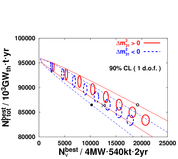
Figure 4: The contours which surround the region consistent with CP conservation are plotted in the number-of-events space of reactor and the LBL experiments. The thin lines correspond to $\delta^{\text{best}}=\pm\pi/2$. The three symbols, a cross, open and solid circles are placed on the figures as well as in Fig. 3 to indicate the relationship between observed numbers of events and the results of CP sensitivity analysis.

The results can be confusing and some of the readers might have naively interpreted, by combining Figs. 3a and 3b, that there is no sensitivity region in $\delta^{\text{best}}\mbox{-}\sin^{2}{2\theta_{23}^{\text{best}}}$ plane. To resolve the puzzling feature we present in Fig. 4 the regions which are consistent with CP conservation by contours in the plane spanned by observable quantities, the number of events in the reactor and the JPARC-HK $\nu_{e}$ appearance experiments. This plot indicates that the sensitivity region for detecting CP violation does not disappear but becomes about half. Which region of $\delta$ is CP sensitive depend upon the sign of $\Delta m^{2}_{13}$, or in other word on the location in bi-number of event plane in Fig. 4. For complete clarity, we have placed three different symbols in Fig. 4 and at the same time in Fig. 3 to indicate which points in the space of observables correspond to which points in the CP sensitivity plot. Note that the point indicated by a cross in Fig. 4 corresponds to two values of $\delta^{\text{best}}$ because of unknown sign of $\Delta m^{2}_{13}$.

V Concluding remarks

In this paper we have pointed out a new method for detecting leptonic CP violation by combining reactor measurement of $\theta_{13}$ with high-statistics $\nu_{e}$ appearance measurement in LBL accelerator experiments. A salient feature of our method are that one can perform the measurement prior to the lengthy antineutrino running in LBL experiments. We conclude with several remarks:

(1) If $\theta_{23}$ is not maximal the parameter degeneracy due to the octant ambiguity of $\theta_{23}$ will also affect the sensitivity of detecting CP violation. On the other hand, we have discussed in our previous communication MSYIS that the octant degeneracy may be resolved by combining reactor measurement of $\theta_{13}$ with the LBL appearance measurement in both neutrino and antineutrino channels. It would be very interesting to reexamine the possibility in the context of this work to clarify to what extent it cures the further uncertainty in the sensitivity of detecting CP violation mentioned above.

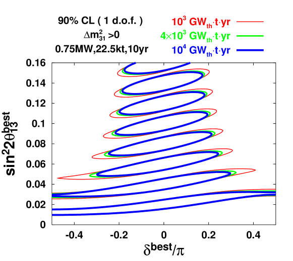
Figure 5: The same as in Fig. 2 but with measurement in 10 years running of the JPARC-SK experiment with 0.75MW beam power and 22.5kt detector (Super-Kamiokande). Although each contour becomes thicker because of a factor of $\simeq$ 25 lower statistics of the experiment, the sensitivity to CP violation still exists at 90% CL.

(2) We have examined a pessimistic scenario to run the JPARC-SK experiment with 0.75MW proton beam power and the fiducial volume of 22.5kt, while waiting for the construction of Hyper-Kamiokande. As is shown in Fig. 5 the sensitivity to CP violation becomes worse but still remains for its 10 years running.

(3) The reactor experiment described in this paper may be regarded as the phase II of the currently proposed reactor experiments for measuring $\theta_{13}$ krasnoyarsk ; kashkari ; diablo , and how to improve the systematic errors should be carefully investigated during running the phase I experiments. If it is possible to significantly improve the systematic errors over those given in Table 1, it may be possible to extend the CP sensitivity to the region $\sin^{2}{2\theta_{13}}\leq 0.03$.

(4) From Figs. 2-3, it is likely that detection of CP violation requires $\sim 10^{3}$ $\text{GW}_{\text{th}}\cdot\mbox{ton}\cdot\mbox{year}$ measurement by the reactor experiment. Now there is a choice between two options: stronger power source with smaller detectors, or weaker power source with larger detectors. If these is no natural or existing holes with enough overburden for the detectors the first option might be more advantageous because larger detectors require deeper hole to keep the signal to noise ratio equal.

Appendix A Cancellation of errors by near-far detector comparison

This appendix is meant to be a pedagogical note in which we try to clarify the feature of cancellation of systematic errors by near-far detector comparison and the relationship between over-all and bin-by-bin errors.

The definition of $\Delta\chi^{2}$ for two detector system is

$$\Delta\chi_{nf}^{2} \equiv \min_{\alpha}\Delta\chi_{nf}^{2}(\alpha)$$ (20)

$$\equiv \min_{\alpha}\left[\frac{\left\{N_{f}-(1+\alpha)N_{f}^{\text{best}}\right\}^{2}}{N_{f}^{\text{best}}+\sigma_{\text{d}}^{2}(N_{f}^{\text{best}})^{2}}+\frac{\left\{N_{n}-(1+\alpha)N_{n}^{\text{best}}\right\}^{2}}{N_{n}^{\text{best}}+\sigma_{\text{d}}^{2}(N_{n}^{\text{best}})^{2}}+\frac{\alpha^{2}}{\sigma_{\text{D}}^{2}}\right],$$

where $N_{f}$ ($N_{n}$) is the theoretical total number of events expected to be measured at far (near) detector. The quantities with superscript “best” are defined as the ones calculated with the best-fit values of the “experimental data”, which are to be tested against the CP conserving case. $\sigma_{\text{D}}$ and $\sigma_{\text{d}}$ are correlated and uncorrelated errors between detectors, respectively.

We discuss statistical average of an observable $O$ by the Gaussian probability distribution function as

$$<O>\equiv C\int dN_{f}dN_{n}d\alpha\,O\exp\left(-\frac{1}{\,2\,}\Delta\chi_{nf}^{2}(\alpha)\right),$$ (21)

where $C$ is the normalization constant to make $<1>$ unity. Note that the integration with respect to $\alpha$ is equivalent to the minimization in (20). After the minimization, it takes the following form which is generic to the Gaussian distribution,

$$\Delta\chi_{nf}^{2} = \left(x,y\right)\left(\begin{array}[]{cc}<x^{2}>&<xy>\\ <yx>&<y^{2}>\end{array}\right)^{-1}\left(\begin{array}[]{c}x\\ y\end{array}\right),$$ (26)

$$x \equiv \frac{N_{f}-N_{f}^{\text{best}}}{N_{f}^{\text{best}}},\ \ y\equiv\frac{N_{n}-N_{n}^{\text{best}}}{N_{n}^{\text{best}}}.$$ (27)

In order to examine the feature of near-far cancellation of errors, it is valuable to transform $x$ and $y$ as

$$X\equiv x-y=\frac{N_{f}}{N_{f}^{\text{best}}}-\frac{N_{n}}{N_{n}^{\text{best}}},\ \ \ Y\equiv x+y=\frac{N_{f}}{N_{f}^{\text{best}}}+\frac{N_{n}}{N_{n}^{\text{best}}}-2.$$ (28)

Then, $\Delta\chi_{nf}^{2}$ can be written as in the form (26) with

$$<X^{2}> = \frac{1}{N_{f}^{\text{best}}}+\frac{1}{N_{n}^{\text{best}}}+2\sigma_{\text{d}}^{2},$$ (29)

$$<Y^{2}> = \frac{1}{N_{f}^{\text{best}}}+\frac{1}{N_{n}^{\text{best}}}+2\sigma_{\text{d}}^{2}+4\sigma_{\text{D}}^{2},$$ (30)

$$<XY> = <YX>=\frac{1}{N_{f}^{\text{best}}}-\frac{1}{N_{n}^{\text{best}}}.$$ (31)

It is evident in (29) that the correlated systematic errors cancel by the near-far comparison. The systematic error $\sqrt{2}\sigma_{\text{d}}$ in $<X^{2}>$ is referred in MSYIS ; bugey as the relative normalization error.

We briefly treat the case of two bins with infinite statistics to illustrate the importance of uncorrelated errors. In this case $X$ subspace of $\Delta\chi^{2}_{nf}$ can be written as

$$X(2\sigma_{d}^{2})^{-1}X\ \longrightarrow\ \left(X_{1},X_{2}\right)\left(\begin{array}[]{cc}2\sigma_{\text{dB}}^{2}+2\sigma_{\text{db}}^{2}&2\sigma_{\text{dB}}^{2}\\ 2\sigma_{\text{dB}}^{2}&2\sigma_{\text{dB}}^{2}+2\sigma_{\text{db}}^{2}\end{array}\right)^{-1}\left(\begin{array}[]{c}X_{1}\\ X_{2}\end{array}\right).$$ (36)

It is clear that $\sigma_{\text{db}}=0$ leads to the diverge of $\Delta\chi_{nf}^{2}$ except for the best fit point ($X_{i}=Y_{i}=0$), which means that the infinite precision can be achieved for the case. Thus, $\sigma_{\text{db}}$ must be treated with great care.

Next we derive the relationship between over-all and bin-by-bin errors that was used in the text, (8). For simplicity, we consider the case of one detector with two bins. Then, $\Delta\chi^{2}$ for the case is defined as

$$\Delta\chi_{12}^{2} \equiv \min_{\alpha}\Delta\chi_{12}^{2}(\alpha)$$ (37)

$$\equiv \min_{\alpha}\left[\frac{\left\{N_{1}-(1+\alpha)N_{1}^{\text{best}}\right\}^{2}}{N_{1}^{\text{best}}+\sigma_{\text{b}}^{2}(N_{1}^{\text{best}})^{2}}+\frac{\left\{N_{2}-(1+\alpha)N_{2}^{\text{best}}\right\}^{2}}{N_{2}^{\text{best}}+\sigma_{\text{b}}^{2}(N_{2}^{\text{best}})^{2}}+\frac{\alpha^{2}}{\sigma_{\text{B}}^{2}}\right],$$

where $N_{1}$ and $N_{2}$ are the expected numbers of events within first and second bins, respectively, and $\sigma_{\text{B}}$ ($\sigma_{\text{b}}$) denotes the correlated (uncorrelated) error between bins.

To obtain the error for the total number of events, we define

$$x_{\text{tot}}\equiv\sum_{i}\frac{N_{i}-N_{i}^{\text{best}}}{N_{\text{tot}}^{\text{best}}},\ \ N_{\text{tot}}^{\text{best}}\equiv\sum_{i}N_{i}^{\text{best}}.$$ (38)

Then, we obtain

$$<x_{\text{tot}}^{2}> = C^{\prime}\int dN_{1}dN_{2}d\alpha\,x_{\text{tot}}^{2}\exp\left(-\frac{1}{\,2\,}\Delta\chi_{12}^{2}(\alpha)\right)$$ (39)

$$= \frac{1}{N_{\text{tot}}^{\text{best}}}+\sigma_{\text{B}}^{2}+\sigma_{\text{b}}^{2}\frac{\sum_{i}(N_{i}^{\text{best}})^{2}}{(N_{\text{tot}}^{\text{best}})^{2}}.$$

One can show that the same treatment goes though for arbitrary number of bins. The coefficient of $\sigma_{\text{b}}^{2}$ is almost 1/9 in our analysis (14 bins).

References

- (1) Y. Fukuda et al. [Kamiokande Collaboration], Phys. Lett. B 335, 237 (1994); Y. Fukuda et al. [Super-Kamiokande Collaboration], Phys. Rev. Lett. 81, 1562 (1998) [arXiv:hep-ex/9807003]; S. Fukuda et al. [Super-Kamiokande Collaboration], Phys. Rev. Lett. 85, 3999 (2000) [arXiv:hep-ex/0009001].
- (2) B. T. Cleveland et al., Astrophys. J. 496, 505 (1998); J. N. Abdurashitov et al. [SAGE Collaboration], Phys. Rev. C 60, 055801 (1999) [arXiv:astro-ph/9907113]; W. Hampel et al. [GALLEX Collaboration], Phys. Lett. B 447, 127 (1999); S. Fukuda et al. [Super-Kamiokande Collaboration], Phys. Rev. Lett. 86, 5651 (2001) [arXiv:hep-ex/0103032]; ibid. 86, 5656 (2001) [arXiv:hep-ex/0103033]; Q. R. Ahmad et al. [SNO Collaboration], Phys. Rev. Lett. 87, 071301 (2001) [arXiv:nucl-ex/0106015]; ibid. 89, 011301 (2002) [arXiv:nucl-ex/0204008]; ibid. 89, 011302 (2002) [arXiv:nucl-ex/0204009].
- (3) S. H. Ahn et al. [K2K Collaboration], Phys. Lett. B 511, 178 (2001) [arXiv:hep-ex/0103001]; M. H. Ahn et al. [K2K Collaboration], Phys. Rev. Lett. 90, 041801 (2003) [arXiv:hep-ex/0212007].
- (4) K. Eguchi et al. [KamLAND Collaboration], Phys. Rev. Lett. 90, 021802 (2003) [arXiv:hep-ex/0212021].
- (5) Z. Maki, M. Nakagawa and S. Sakata, Prog. Theor. Phys. 28, 870 (1962).
- (6) M. Apollonio et al. [CHOOZ Collaboration], Phys. Lett. B 420, 397 (1998) [arXiv:hep-ex/9711002]; ibid. B 466, 415 (1999) [arXiv:hep-ex/9907037]. See also, The Palo Verde Collaboration, F. Boehm et al., Phys. Rev. D 64 (2001) 112001 [arXiv:hep-ex/0107009].
- (7) M. Kobayashi and T. Maskawa, Prog. Theor. Phys. 49, 652 (1973).
-
(8)
Y. Itow et al., arXiv:hep-ex/0106019.
For an updated version, see: http://neutrino.kek.jp/jhfnu/loi/loi.v2.030528.pdf - (9) D. Ayres et al. arXiv:hep-ex/0210005.
- (10) J. J. Gomez-Cadenas et al. [CERN working group on Super Beams Collaboration] arXiv:hep-ph/0105297.
- (11) M. Diwan et al. [Report of BNL Neutrino Working Group] arXiv:hep-ex/0211001.
- (12) C. Albright et al., arXiv:hep-ex/0008064; M. Apollonio et al., arXiv:hep-ph/0210192.
- (13) For early ideas of superbeam experiments, see H. Minakata and H. Nunokawa, Phys. Lett. B495 (2000) 369; [arXiv:hep-ph/0004114]; J. Sato, Nucl. Instrum. Meth. A472 (2001) 434 [arXiv:hep-ph/0008056]; B. Richter, arXiv:hep-ph/0008222.
- (14) J. Burguet-Castell, M. B. Gavela, J. J. Gomez-Cadenas, P. Hernandez and O. Mena, Nucl. Phys. B 608, 301 (2001) [arXiv:hep-ph/0103258].
- (15) H. Minakata and H. Nunokawa, JHEP 0110, 001 (2001) [arXiv:hep-ph/0108085]; Nucl. Phys. Proc. Suppl. 110, 404 (2002) [arXiv:hep-ph/0111131].
- (16) T. Kajita, H. Minakata and H. Nunokawa, Phys. Lett. B 528, 245 (2002) [arXiv:hep-ph/0112345].
- (17) G. Fogli and E. Lisi, Phys. Rev. D54, 3667 (1996); [arXiv:hep-ph/9604415].
- (18) V. Barger, D. Marfatia and K. Whisnant, Phys. Rev. D 65, 073023 (2002) [arXiv:hep-ph/0112119];
- (19) H. Minakata, H. Nunokawa, and S. J. Parke, Phys. Rev. D 66, 093012 (2002) [arXiv:hep-ph/0208163].
- (20) H. Minakata, H. Sugiyama, O. Yasuda, K. Inoue, and F. Suekane, Phys. Rev. D 68, 033017 (2003). [arXiv:hep-ph/0211111].
- (21) P. Huber, M. Lindner, T. Schwetz and W. Winter, Nucl. Phys. B 665, 487 (2003) [arXiv:hep-ph/0303232].
-
(22)
Y. Kozlov, L. Mikaelyan and V. Sinev, arXiv:hep-ph/0109277;
V. Martemyanov, L. Mikaelyan, V. Sinev, V. Kopeikin, and Y. Kozlov, arXiv:hep-ex/0211070. - (23) F. Suekane, K. Inoue, T. Araki, and K. Jongok, arXiv:hep-ex/0306029, to appear in Proceedings of The Fourth Workshop on Neutrino Oscillations and Their Origin (NOON2003), to be published by World Scientific.
-
(24)
M. A. Shaevitz and J. M. Link,
arXiv:hep-ex/0306031, to appear in
Proceedings of NOON2003.
For other projects, see the webpage of Workshop on Future Low-Energy Neutrino Experiments, April 30-May 2, University of Alabama, Tuscaloosa, Alabama;
http://bama.ua.edu/ busenitz/reactornu2003.html - (25) A. Cervera, A. Donini, M. B. Gavela, J. J. Gomez Cadenas, P. Hernandez, O. Mena and S. Rigolin, Nucl. Phys. B579 (2000) 17 [arXiv:hep-ph/0002108]. [Erratum-ibid. B593 (2000) 731].
- (26) K. Hagiwara et al. [Particle Data Group Collaboration], Phys. Rev. D 66, 010001 (2002).
- (27) M. Shiozawa, Talk at Eighth International Workshop on Topics in Astroparticle and Underground Physics (TAUP2003), September 5-9, 2003, Seattle, Washington.
- (28) J. Kameda, Detailed Studies of Neutrino Oscillation with Atmospheric Neutrinos of Wide Energy Range from 100 MeV to 1000 GeV in Super-Kamiokande, Ph. D thesis, University of Tokyo, September 2002.
- (29) T. Kobayashi, private communications.
- (30) H. Sugiyama, O. Yasuda, F. Suekane, and G. A. Horton-Smith, in preparation.
- (31) D. Stump et al. Phys. Rev. D 65, 014012 (2002) [arXiv:hep-ph/0101051].
- (32) M. B. Smy et al. [Super-Kamiokande Collaboration], arXiv:hep-ex/0309011.
- (33) S. N. Ahmed et al. [SNO Collaboration], arXiv:nucl-ex/0309004.
- (34) M. Koike and J. Sato, Mod. Phys. Lett. A14, 1297 (1999) [arXiv:hep-ph/9803212].
- (35) G. L. Fogli, E. Lisi, A. Marrone, D. Montanino, A. Palazzo, and A. M. Rotunno, arXiv:hep-ph/0308055.
- (36) Y. Hayato, Talk at International Europhysics Conference on High Energy Physics (EPS2003), July 17-23, 2003, Aachen, Germany.
- (37) Y. Declais et al., Nucl. Phys. B 434, 503 (1995).