Electroweak $2\rightarrow 2$ amplitudes for electron-positron annihilation at TeV energies

Abstract

The non-radiative scattering amplitudes for electron-positron annihilation into quark and lepton pairs in the TeV energy range are calculated in the double-logarithmic approximation. The expressions for the amplitudes are obtained using infrared evolution equations with different cut-offs for virtual photons and for $W$ and $Z$ bosons, and compared with previous results obtained with an universal cut-off.

I Introduction

Next future linear $e^{+}e^{-}$ colliders will be operating in a energy domain which is much higher than the electroweak bosons masses, so that the full knowledge of the scattering amplitudes for $e^{+}e^{-}$ annihilation into quark and lepton pairs will be needed. The forward-backward asymmetry for $e^{+}e^{-}$ annihilation into leptons or hadrons produced at energies much greater than the $W$ and $Z$ boson masses has been recently considered in Ref. egt , where the electroweak radiative corrections were calculated to all orders in the double-logarithmic approximation (DLA). It was shown that the effect of the electroweak DL radiative corrections on the value of the forward-backward asymmetry is quite sizable and grows rapidly with the energy. As usual, the asymmetry is defined as the difference between the forward and the backward scattering amplitudes over the sum of them. These amplitudes were calculated in Ref. egt in DLA, by introducing and solving the Infrared Evolution Equations (IREE). This method is a very simple and the most efficient instrument for performing all-orders double-logarithmic calculations (see Ref. flmm and Refs. therein). In particular, when it was applied in Ref. flmm to calculate the electroweak Sudakov (infrared-divergent) logarithms, it led easily to the proof of the exponentiation of the Sudakov logarithms. At that moment this was in contradiction to the non-exponentiation claimed in Ref. pciaf and obtained by other means. This contradiction provoked a large discussion about the exponentiation. The exponentiation was confirmed eventually by the two-loop calculations in Refs. me -dp and by summing up the higher loop DL contributions in Refs. kp and m . These Sudakov logarithms provide the whole set of DL contributions to the $2\to 2$ amplitudes only when the process is considered in the hard kinematic region where all the Mandelstam variables $s,t,u$ are of the same order. On the other hand, when the kinematics of the $2\to 2$ processes is of the Regge type, besides the Sudakov logarithms, another kind of DL contributions arises, coming from ladder Feynman graphs. Accounting for those (infrared stable) contributions it leads, instead of simple exponentials, to much more complicated expressions for the scattering amplitudes. This was first shown in Ref. ggfl , where in the framework of pure QED, the scattering amplitudes for the forward and backward $e^{+}e^{-}\to\mu^{+}\mu^{-}$ annihilation were calculated in the Regge kinematics. One example of high-energy electroweak processes in the Regge kinematics was considered in Ref. flmm , where the backward scattering amplitude was calculated, for the annihilation of a lepton pair with same helicities into another pair of leptons. More general calculations of the forward and backward electroweak scattering amplitudes were done in Ref egt .

However, both calculations in Refs. egt and  flmm were done under the assumption that the transverse momenta $k_{i\perp}$ of the virtual photons and virtual $W,Z$ -bosons were much greater than the masses of the weak bosons. In other words, the same infrared cut-off $M$ in the transverse momentum space, was used for all virtual electroweak bosons, i.e.,

$$k_{i\perp}\gg M\geq M_{W}\approx M_{Z}.$$ (1)

Obviously, while $M$ is the natural infrared cut-off for the logarithmic contributions involving $W,Z$ bosons, the cut-off for the photons can be chosen independently. in accord with the experimental resolution in a given observed process. Indeed the assumption (1), although simplifying the calculations a lot, is unnecessary and an approach that involves different cut-offs for photons and $W,Z$ weak bosons would be more interesting and suitable for phenomenological applications. This technique involving different cut-offs for photons and for $W,Z$ bosons was applied in Ref. flmm , for calculating the double-logarithmic contributions of soft virtual electroweak bosons (the Sudakov electroweak logarithms) but not for the scattering amplitudes in the regions of Regge kinematics.

In the present paper we generalize the results of Refs. flmm and  egt , and obtain new double-logarithmic expressions for the $2\to 2$ - electroweak amplitudes in the forward and backward kinematics. These expressions involve therefore different infrared cut-offs for virtual photons and virtual weak bosons. Throughout the paper we assume that the photon cut-off, $\mu$, and the $W,Z$ boson cut-off, $M$, satisfy the relations

$$M\geq M_{W,Z},~{}~{}~{}\mu\geq m_{f}$$ (2)

where $m_{f}$ is the largest mass of the quarks or leptons involved in the process. Notice that the values of $M$ and $\mu$ could be widely different. Let us remind that in order to study a scattering amplitude $A(s,t)$ in the Regge kinematics $s\gg-t$ (where $s$ and $t$ are the standard Mandelstam variables), it is convenient to represent $A(s,t)$ in the following form: $A(s,t)=A^{(+)}(s,t)+A^{(-)}(s,t)$, with $A^{(\pm)}(s,t)=(1/2)[A(s,t)\pm A(-s,t)]$ called the positive (negative) signature amplitudes. We shall consider only amplitudes with the positive signatures. The IREE for the negative signature electroweak amplitudes can be obtained in a similar way, see e.g. Ref. egt for more details.

The paper is organized as follows: in Sect. 2 we define the kinematics and express the scattering amplitude for the $e^{+}e^{-}$ annihilation in terms of invariant amplitudes. In Sect. 3, we construct the evolution equations for the invariant amplitudes for the case when in the center mass (cm) frame, the scattering angles are very small. First, we obtain the IREE equations in the integral form and then we transform them in the simpler, differential form. These differential equations are solved in Sect. 4 and explicit expressions for the invariant amplitudes involving the Mellin integrals are obtained. In Sect. 5, we consider the case of large scattering angles, or when the Mandelstam variables s, t and u are all large. Sect. 6 deals with the expansion of the invariant amplitudes into the perturbative series in order to extract the first-loop and the second-loop contributions. Then we compare these contributions to the analogous terms obtained when one universal cut-off is used and study their difference. The effect of high-order contributions in the two approaches is further studied in Sect. 7 where the asymptotic expressions of the amplitudes are compared. Finally, Sect. 8 contains our concluding remarks.

II Invariant amplitudes for the annihilation processes

Let us consider a general process where the lepton $l^{k}(p_{1})$ and its anti-particle $\bar{l}_{i}(p_{2})$ annihilate into a quark or a lepton $q^{k^{\prime}}(p^{\prime}_{1})$ and its anti-particle $\bar{q}_{i^{\prime}}({p^{\prime}}_{2})$ (see Fig. 1):

$$l^{k}(p_{1})\bar{l}_{i}(p_{2})\to q^{k^{\prime}}({p^{\prime}}_{1})\bar{q}_{i^{\prime}}({p^{\prime}}_{2})~{}.$$ (3)

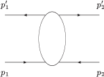
Figure 1: Scattering amplitude of the annihilation of Eq. 3.

For this process, the most complicate case occurs when both the initial and the final particles (anti-particles) are left-handed (right-handed). The scattering amplitudes for other helicities can be obtained easily from the formulae derived for this case. As there is no technical difference when considering the annihilation into quarks or leptons, we present parallel results for the annihilation into a quark-antiquark or a lepton-antilepton pair. According to our assumption, the initial lepton belongs to the weak isodoublet $(\nu,~{}e)$. The final lepton belongs to another doublet, e.g. $(\nu_{\mu},~{}\mu)$, and the final quarks are also from a doublet, e.g. $(u,~{}d)$. The antilepton and the antiquark belong to the charge conjugate doublets. Obviously, the scattering amplitude $A$ for the annihilation can be written as follows:

$$A=q^{k^{\prime}}({p^{\prime}}_{1})\bar{q}_{i^{\prime}}({p^{\prime}}_{2})A^{ii^{\prime}}_{k^{\prime}k}l^{k}(p_{1})\bar{l}_{i}(p_{2})~{},$$ (4)

where the $SU(2)$ matrix amplitude $A^{ii^{\prime}}_{k^{\prime}k}$ has to be calculated. We will consider it in DLA. The DL contributions to $A^{ii^{\prime}}_{k^{\prime}k}$ are different according to the kinematics of the process. The kinematics is defined by appropriate relations among the Mandelstam variables $s,~{}t,~{}u$,

$$s=(p_{1}+p_{2})^{2},~{}t=(p_{1}-{p^{\prime}}_{1})^{2},~{}u=(p_{1}-{p^{\prime}}_{2})^{2}~{}.$$ (5)

Throughout this paper we assume that $\sqrt{s}\gg M_{W,Z}$.

The kinematical regime defined as

$$-t\sim-u\sim s$$ (6)

is called the hard kinematics and corresponds to large cm scattering angles $\theta\equiv\theta_{\mathbf{p_{1}\,{p^{\prime}}_{1}}}\sim 1$ . Radiative corrections to the annihilation in this kinematics yield DL contributions.

There are also two other Regge-type kinematical regimes where DL contributions appear. First, there is the configuration where

$$s\sim-u\gg-t~{}.$$ (7)

We call it the $t$ -kinematics. According to the terminology introduced in ggfl , it is the forward kinematics (with respect to the charge flow) for $e^{+}e^{-}\to\mu^{+}\mu^{-}$ and $e^{+}e^{-}\to d\bar{d}$. At the same time, it corresponds to the backward kinematics for $e^{+}e^{-}\to u\bar{u}$. In this kinematics, $\theta\ll 1$.

Second, there is the opposite kinematics where $\theta\sim\pi$ and therefore

$$s\sim-t\gg-u~{}.$$ (8)

We define the configuration (8) as the $u$-kinematics. It corresponds to the forward scattering for $e^{+}e^{-}\to u\bar{u}$ and the backward scattering for $e^{+}e^{-}\to\mu^{+}\mu^{-}$,  $e^{+}e^{-}\to d\bar{d}$.

To simplify the calculations, it is convenient to introduce the projection operators $(P_{j})^{ii^{\prime}}_{k^{\prime}k}~{}(j=1,2,3,4)$, so that $A^{ii^{\prime}}_{k^{\prime}k}$ can be written in the following form:

$$A^{ii^{\prime}}_{k^{\prime}k}=\frac{\bar{u}(-{p^{\prime}}_{2})\gamma_{\mu}u({p^{\prime}}_{1})\bar{u}(-p_{2})\gamma^{\mu}u(p_{1})}{s}|\Big{[}(P_{j})_{kk^{\prime}}^{ii^{\prime}}A_{j}+(P_{j+1})_{kk^{\prime}}^{ii^{\prime}}A_{j+1}\Big{]}~{},$$ (9)

where $j=1$ for the $t$-kinematics and $j=3$ for the $u$-kinematics. The representation (9) reduces the calculation of the matrix amplitude $A^{ii^{\prime}}_{k^{\prime}k}$ to the calculation of the invariant amplitudes $A_{j}$. The explicit expressions for the operators $(P_{c})^{ii^{\prime}}_{k^{\prime}k}~{}(c=1,..,4)$ can be taken from Ref. egt :

$$(P_{1})_{kk^{\prime}}^{ii^{\prime}}=\frac{1}{2}\delta_{k}^{i^{\prime}}\delta^{i}_{k^{\prime}}, (P_{2})_{kk^{\prime}}^{ii^{\prime}}=2(t_{c})_{k}^{i}(t_{c})^{i^{\prime}}_{k^{\prime}},$$ (10)

$$(P_{3})_{kk^{\prime}}^{ii^{\prime}}=\frac{1}{2}\left[\delta^{i}_{k}\delta^{i^{\prime}}_{k^{\prime}}-\delta^{i^{\prime}}_{k}\delta^{i}_{k^{\prime}}\right]~{}, (P_{4})_{kk^{\prime}}^{ii^{\prime}}=\frac{1}{2}\left[\delta^{i}_{k}\delta_{k^{\prime}}^{i^{\prime}}+\delta^{i^{\prime}}_{k}\delta^{i}_{k^{\prime}}\right]~{}.$$

According to the results of Ref. egt , the forward $(A_{F})$ and backward $(A_{B})$ amplitudes of the $e^{+}e^{-}$ annihilation into quarks are expressed through invariant amplitudes $A_{j}$ as follows:

$$A_{F}(e^{+}e^{-}\to u\bar{u})=(A_{3}+A_{4})/2,~{}A_{B}(e^{+}e^{-}\to u\bar{u})=A_{4},$$ (11)

$$~{}A_{F}(e^{+}e^{-}\to d\bar{d})=(A_{1}+A_{2})/2,~{}A_{B}(e^{+}e^{-}\to d\bar{d})=A_{2}~{}.$$

and the annihilation into leptons is expressed through the leptonic invariant amplitudes very similarly:

$$A_{F}(e^{+}e^{-}\to\mu^{+}\mu^{-})=(A_{1}+A_{2})/2,~{}A_{B}(e^{+}e^{-}\to\mu^{+}\mu^{-})=A_{2}~{},$$ (12)

$$A_{F}(e^{+}e^{-}\to\nu_{\mu}\bar{\nu_{\mu}})=(A_{3}+A_{4})/2,~{}~{}A_{B}(e^{+}e^{-}\to\nu_{\mu}\bar{\nu_{\mu}})=A_{4}~{}.$$

We have used the general notation $A_{j}$ for the invariant amplitudes in Eqs. (11, 12) and we will keep using this notation until Sect. 4.

In order to calculate the amplitudes $A_{j}$ to all orders in the electroweak couplings in the DLA, we construct and solve some infrared evolution equations (IREE). These equations describe the evolution of $A_{j},~{}(j=1,2,3,4)$ with respect to an infrared cut-off. We introduce two such cut-offs, $\mu$ and $M$. We presume that $M\approx M_{Z}\approx M_{W}$ and use this cut-off to regulate the DL contributions involving soft (almost on-shell) virtual $W,Z$ -bosons. In order to regulate the IR divergences arising from soft photons we use the cut-off $\mu$ and we assume that $\mu\approx m_{q}\ll M$ where $m_{q}$ is the maximal quark mass involved. Both cut-offs are introduced in the transverse momentum space (with respect to the plane formed by momenta of the initial leptons) so that the transverse momenta $k_{i}$ of virtual photons obey

$$k_{i\perp}>\mu~{},$$ (13)

while the momenta $k_{i}$ of virtual $W,Z$ -bosons obey

$$k_{i\perp}>M~{}.$$ (14)

Let us first consider $A_{j}$ in the collinear kinematics where, in the cm frame, the produced quarks or leptons move very close to the $e^{+}e^{-}$ -beams. In order to fix such kinematics, we implement Eq. (7) by the further restriction on $t$:

$$s\sim-u\gg M^{2}\gg\mu^{2}\geq-t$$ (15)

and similarly for Eq. (8) by

$$s\sim-t\gg M^{2}\gg\mu^{2}\geq-u~{}.$$ (16)

Basically in DLA, the invariant amplitudes $A_{j}$ depend on $s,u$ and $t$ through logarithms. Under the restriction imposed by Eqs. (15, 16) then all $A_{j}$ depend only on logarithms of $s,M^{2},\mu^{2}$ in the collinear kinematics. It is convenient to represent $A_{j}$ in the following form:

$$A_{j}(s,\mu^{2},M^{2})=A_{j}^{(QED)}(s,\mu^{2})+{A^{\prime}}_{j}(s,\mu^{2},M^{2})~{},$$ (17)

where $A_{j}^{(QED)}(s,\mu^{2})$ accounts for QED DL contributions only, i.e. the contributions of Feynman graphs without virtual $W,Z$ bosons. To calculate $A_{j}^{(QED)}(s,\mu^{2})$ we use the cut-off $\mu$, therefore the amplitudes $A_{j}^{(QED)}$ do not depend on $M$. In contrast, the amplitudes ${A^{\prime}}_{j}(s,\mu^{2},M^{2})$ depend on both cut-offs. These amplitudes account for DL contributions of the Feynman graphs, with one or more $W,Z$ propagators. By technical reasons, it is convenient to introduce two auxiliary amplitudes. The first one, $\tilde{A}^{(QED)}_{j}(s,M^{2})$, is the same QED amplitude but with a cut-off $M$. The second auxiliary amplitude, $\tilde{A}_{j}(s,M^{2})$ accounts for all electroweak DL contributions and the cut-off $M$ is used to regulate both the virtual photons and the weak bosons infrared divergences.

Beyond the Born approximation, the invariant amplitudes we have introduced depend on logarithms, the arguments of which can be chosen as in the following parameterization:

$$A_{j}^{(QED)}=A_{j}^{(QED)}(s,\mu^{2})=A_{j}^{(QED)}(s/\mu^{2}),~{}\tilde{A}^{(QED)}_{j}=\tilde{A}^{(QED)}_{j}(s,M^{2})=\tilde{A}^{(QED)}_{j}(s/M^{2}),$$ (18)

$$~{}\tilde{A}_{j}=\tilde{A}_{j}(s,M^{2})=\tilde{A}_{j}(s/M^{2}),~{}{A^{\prime}}_{j}={A^{\prime}}_{j}(s,\mu^{2},M^{2})={A^{\prime}}_{j}(s/M^{2},\eta)~{},$$

with

$$\eta\equiv\ln(M^{2}/\mu^{2})~{}.$$ (19)

Our aim is to calculate the amplitudes ${A^{\prime}}_{j}$, whereas the amplitudes $A_{j}^{(QED)},\tilde{A}^{(QED)}_{j}$ and $\tilde{A}_{j}(s/M^{2})$ are supposed to be known. The amplitudes $\tilde{A}_{j}$ were introduced and calculated in Ref. egt . In order to define amplitudes ${A^{\prime}}_{j},\tilde{A}_{j}(s,M^{2})$, the projection operators of Eq. (10) have been used. The use of these operators is based on the fact that the $SU(2)\times U(1)$ symmetry for the electroweak scattering amplitudes takes place at energies much higher than the weak mass scale $M$. On the contrary, the QED amplitudes $A_{j}^{(QED)}$ and $\tilde{A}^{(QED)}_{j}$ are not $SU(2)$ invariant at any energy. Nevertheless, it is convenient to introduce “the QED invariant amplitudes” $A_{j}^{(QED)},\tilde{A}^{(QED)}_{j}$ by explicit calculation of the forward and backward QED scattering amplitudes. Then inverting Eq. (11), we construct the amplitudes $A_{j}^{(QED)}$ for $e^{+}e^{-}$- annihilation into quarks:

$$A_{1}^{(QED)}=2A_{F}^{(QED)}(e^{+}e-\to d\bar{d})-A_{B}^{(QED)}(e^{+}e-\to u\bar{u}),~{}~{}A_{2}^{(QED)}=A_{B}^{(QED)}(e^{+}e-\to u\bar{u}),$$ (20)

$$A_{3}^{(QED)}=2A_{F}^{(QED)}(e^{+}e-\to u\bar{u})-A_{B}^{(QED)}(e^{+}e-\to d\bar{d}),~{}~{}A_{4}^{(QED)}=A_{B}^{(QED)}(e^{+}e-\to d\bar{d})~{}$$

and inverting Eq. (12) allows us to obtain $A_{j}^{(QED)}$ for $e^{+}e^{-}$- annihilation into leptons:

$$A_{1}^{(QED)}=2A_{F}^{(QED)}(e^{+}e-\to\mu^{+}\mu^{-}),~{}A_{2}^{(QED)}=0,~{}A_{3}^{(QED)}=-A_{4}^{(QED)}=A_{B}^{(QED)}(e^{+}e-\to\mu^{+}\mu^{-}).$$ (21)

III Evolution equations for amplitudes $A_{j}$ in the collinear kinematics

We would like to discuss now the IREE for the amplitudes introduced earlier. The basic idea for constructing infrared evolution equations for the scattering amplitudes consists in introducing the infrared cut-offs in the transverse momentum space and evolving the scattering amplitudes with respect to them. This method does not involve analyzing the DL contributions of specific Feynman graphs but is based on quite general conceptions such as the analyticity of the scattering amplitudes and the dispersion relations which guarantees its applicability to a wide class of problems (see e.g. Ref. flmm and Refs. therein). The essence of the method is the factorizing the DL contributions of virtual particles with the minimal transverse momenta. The IREE with two cut-offs for the electroweak amplitudes in the hard kinematics (6) were obtained in Ref. flmm . In the present section we construct the IREE for the $2\rightarrow 2$ - electroweak amplitudes in the Regge kinematics. According to Eqs. (13, 14), we use two different cut-offs for the virtual photons and for the weak bosons. The amplitude $A_{j}$ is in the lhs of such an equation. The rhs contains several terms. In the first place, there is the Born amplitude $B_{j}$. In order to obtain the other terms in the rhs, we use the fact that the DL contributions of virtual particles with minimal transverse momenta $(\equiv k_{\perp})$ can be factorized. Furthermore, this $k_{\perp}$ acts as a new cut-off for the other virtual momenta. The virtual particle with $k_{\perp}$ (we call such a particle the softest one) can be either an electroweak bosons or a fermion. Let us suppose first that the softest particle is an electroweak boson.

In this case, in the Feynman gauge, DL contributions come from the graphs where the softest propagator is attached to the external lines in every possible way whereas $k_{\perp}$ acts as a new cut-off for the blobs as shown in Fig. 2.

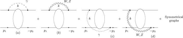
Figure 2: Softest boson contributions to IREE to $A_{j}$.

When the softest electroweak boson is a photon, the integration region over $k_{\perp}$ is $\mu^{2}\ll k_{\perp}^{2}\ll s$ and its contribution, $G^{\gamma}_{j}$, to the rhs of the IREE is:

$$G^{(\gamma)}_{j}=-\frac{1}{8\pi^{2}}b_{j}^{(\gamma)} \Big{(} \int_{\mu^{2}}^{s}\frac{dk_{\perp}^{2}}{k_{\perp}^{2}}\ln(s/k_{\perp}^{2})A^{(QED)}_{j}(s,k_{\perp}^{2})+\int_{\mu^{2}}^{M^{2}}\frac{dk_{\perp}^{2}}{k_{\perp}^{2}}\ln(s/k_{\perp}^{2}){A^{\prime}}_{j}(s,k_{\perp}^{2},M^{2})+$$

$$\int_{M^{2}}^{s}\frac{dk_{\perp}^{2}}{k_{\perp}^{2}}\ln(s/k_{\perp}^{2})A^{\prime}_{j}(s,k_{\perp}^{2},k_{\perp}^{2})\,\Big{)}~{},$$

where

$$b_{1}^{(\gamma)}=g^{2}\sin^{2}\theta_{W}\frac{(Y_{2}-Y_{1})^{2}}{4},~{}~{}~{}b_{2}^{(\gamma)}=g^{2}\sin^{2}\theta_{W}\Big{[}\frac{1}{6}+\frac{(Y_{2}-Y_{1})^{2}}{4}\Big{]}~{},$$ (23)

$$b_{3}^{(\gamma)}=g^{2}\sin^{2}\theta_{W}\frac{(Y_{2}+Y_{1})^{2}}{4},~{}~{}~{}b_{4}^{(\gamma)}=g^{2}\sin^{2}\theta_{W}\Big{[}\frac{1}{6}+\frac{(Y_{2}+Y_{1})^{2}}{4}\Big{]}~{}.$$

We have used the standard notations in Eq. (23): $g,~{}g^{\prime}$ are the Standard Model couplings, $Y_{1}~{}(Y_{2})$ is the hypercharge of the initial (final) fermions and $\theta_{W}$ is the Weinberg angle. The logarithmic factors in the integrands of Eq. (III) correspond to the integration in the longitudinal momentum space. The amplitude $A^{\prime}$ in the last integral of Eq. (III) does not depend on $\mu$ because $k_{\perp}^{2}>M^{2}$. Therefore it can be expressed in terms of $\tilde{A}_{j}(s,k_{\perp}^{2})$ and $\tilde{A}_{j}^{(QED)}(s,k_{\perp}^{2})$ :

$${A^{\prime}}_{j}(s,k_{\perp}^{2},k_{\perp}^{2})=\tilde{A}_{j}(s,k_{\perp}^{2})-\tilde{A}_{j}^{(QED)}(s,k_{\perp}^{2})~{}.$$ (24)

When the softest boson is either a $Z$ or a $W$, its DL contribution can be factorized in the region $M^{2}\ll k_{\perp}^{2}\ll s$. This yields:

$$G_{j}^{(WZ)}=-\frac{1}{8\pi^{2}}b_{j}^{(WZ)}\int_{M^{2}}^{s}\frac{dk_{\perp}^{2}}{k_{\perp}^{2}}\ln(s/k_{\perp}^{2})\tilde{A}_{j}(s/k_{\perp}^{2})~{},$$ (25)

with

$$b_{j}^{(WZ)}=b_{j}-b_{j}^{\gamma}~{}$$ (26)

and the factors $b_{j}$ can be taken from Ref. egt :

$$b_{1}=\frac{{g^{\prime}}^{2}(Y_{1}-Y_{2})^{2}}{4},~{}~{}b_{2}=\frac{8g^{2}+{g^{\prime}}^{2}(Y_{1}-Y_{2})^{2}}{4},$$ (27)

$$~{}~{}b_{3}=\frac{{g^{\prime}}^{2}(Y_{1}+Y_{2})^{2}}{4},~{}~{}b_{4}=\frac{8g^{2}+{g^{\prime}}^{2}(Y_{1}+Y_{2})^{2}}{4}~{}~{}.$$

In Eq. (25) we have used the fact that the $W$ and the $Z$ bosons cannot be the softest particles for the amplitudes $A^{(QED)}_{j}$ since the integrations over the softest transverse momenta in $A^{(QED)}_{j}$ can go down to $\mu$, by definition. The sum of Eqs. (III) and (25) , $G_{j}$ can be written in the more convenient way:

$$G_{j}(s,\mu^{2},M^{2})=G^{(\gamma)}_{j}(s,\mu^{2},M^{2})+G_{j}^{(WZ)}(s,M^{2})=G_{j}^{(QED)}(s,\mu^{2})-\tilde{G}^{(QED)}_{j}(s,M^{2})+\tilde{G}_{j}(s,M^{2})+{G^{\prime}}_{j}(s,\mu^{2},M^{2})~{},$$ (28)

where

$$G^{(QED)}_{j}=-\frac{1}{8\pi^{2}}b_{j}^{(\gamma)}\int_{\mu^{2}}^{s}\frac{dk_{\perp}^{2}}{k_{\perp}^{2}}\ln(s/k_{\perp}^{2})A^{(QED)}_{j}(s/k_{\perp}^{2})~{},\tilde{G}^{(QED)}_{j}=-\frac{1}{8\pi^{2}}b_{j}^{(\gamma)}\int_{M^{2}}^{s}\frac{dk_{\perp}^{2}}{k_{\perp}^{2}}\ln(s/k_{\perp}^{2})\tilde{A}^{(QED)}_{j}(s/k_{\perp}^{2})~{},$$ (29)

$$\tilde{G}_{j}=-\frac{1}{8\pi^{2}}b_{j}\int_{M^{2}}^{s}\frac{dk_{\perp}^{2}}{k_{\perp}^{2}}\ln(s/k_{\perp}^{2})\tilde{A}_{j}(s/k_{\perp}^{2})~{},{G^{\prime}}_{j}=-\frac{1}{8\pi^{2}}b_{j}^{(\gamma)}\int_{\mu^{2}}^{M^{2}}\frac{dk_{\perp}^{2}}{k_{\perp}^{2}}\ln(s/k_{\perp}^{2}){A^{\prime}}_{j}(s/k_{\perp}^{2},M^{2}/k_{\perp}^{2})~{}.$$

Eqs. (28, 29) account for DL contributions when the softest particle is an electroweak boson. However, the softest particle can also be a virtual fermion. In this case, DL contributions from the integration over the momentum $k$ of the softest fermion arise from the diagram shown in Fig. 3 where the amplitudes $A_{j}$ are factorized into two on-shell amplitudes in the $t$-channel. We denote this contribution by $Q_{j}(s,\mu^{2},M^{2})$.

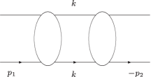
Figure 3: Softest fermion contribution.

The analytic expression for $Q_{j}$ is rather cumbersome. However it looks simpler when the Sudakov parameterization is introduced for the softest quark momentum $k$ (with $p_{1}$ and $p_{2}$ being the initial lepton momenta).

$$k=\alpha p_{2}+\beta p_{1}+k_{\perp}~{}.$$ (30)

After simplifying the spin structure, we obtain

$$Q_{j}(s,\mu^{2},M^{2})=c_{j}\int_{\mu^{2}}^{s}dk_{\perp}^{2}\int\frac{d\alpha}{\alpha}\frac{d\beta}{\beta}\frac{2k_{\perp}^{2}}{(s\alpha\beta-k_{\perp}^{2})^{2}}A_{j}(s\alpha,k_{\perp}^{2},M^{2})A_{j}(s\beta,k_{\perp}^{2},M^{2})~{},$$ (31)

where

$$c_{1}=c_{2}=-c_{3}=-c_{4}=\frac{1}{8\pi^{2}}~{}.$$ (32)

Similarly to Eq. (28), $Q_{j}$ of Eq. (31) can be divided into the following simple contributions:

$$Q_{j}=Q_{j}^{(QED)}-\tilde{Q}_{j}^{(QED)}+\tilde{Q}_{j}+{Q^{\prime}}_{j}~{},$$ (33)

where

$$Q_{j}^{(QED)}(s/\mu^{2})=c_{j}\int_{\mu^{2}}^{s}dk_{\perp}^{2}\int\frac{d\alpha}{\alpha}\frac{d\beta}{\beta}\frac{k_{\perp}^{2}}{(s\alpha\beta-k_{\perp}^{2})^{2}}A_{j}^{(QED)}(s\alpha/k_{\perp}^{2})A_{j}^{(QED)}(s\beta/k_{\perp}^{2})~{},$$ (34)

$$\tilde{Q}_{j}^{(QED)}(s/M^{2})=c_{j}\int_{M^{2}}^{s}dk_{\perp}^{2}\int\frac{d\alpha}{\alpha}\frac{d\beta}{\beta}\frac{k_{\perp}^{2}}{(s\alpha\beta-k_{\perp}^{2})^{2}}\tilde{A}_{j}^{(QED)}(s\alpha/k_{\perp}^{2})\tilde{A}_{j}^{(QED)}(s\beta/k_{\perp}^{2})~{},$$ (35)

$$\tilde{Q}_{j}(s/M^{2})=c_{j}\int_{M^{2}}^{s}dk_{\perp}^{2}\int\frac{d\alpha}{\alpha}\frac{d\beta}{\beta}\frac{k_{\perp}^{2}}{(s\alpha\beta-k_{\perp}^{2})^{2}}\tilde{A}_{j}(s\alpha/k_{\perp}^{2})\tilde{A}_{j}(s\beta/k_{\perp}^{2})~{},$$ (36)

and

$${Q^{\prime}}_{j}(s/M^{2},\eta)=c_{j}\int_{\mu^{2}}^{M^{2}}dk_{\perp}^{2}\int\frac{d\alpha}{\alpha}\frac{d\beta}{\beta}\frac{2k_{\perp}^{2}}{(s\alpha\beta-k_{\perp}^{2})^{2}}\Big{(}2A_{j}^{(QED)}(s\alpha/k_{\perp}^{2}){A^{\prime}}_{j}(s\beta/k_{\perp}^{2},M^{2}/k_{\perp}^{2})$$ (37)

$$+{A^{\prime}}_{j}(s\alpha/k_{\perp}^{2},M^{2}/k_{\perp}^{2}){A^{\prime}}_{j}(s\beta/k_{\perp}^{2},M^{2}/k_{\perp}^{2})\Big{)}~{}.$$

Now we are able to write the IREE for amplitudes $A_{j}$. The general form it given by:

$$A_{j}=B_{j}+G_{j}+Q_{j}~{}.$$ (38)

Then using Eqs. (28) and (33) we can rewrite it as

$${A^{\prime}}_{j}+A_{j}^{(QED)}=B_{j}^{(QED)}-\tilde{B}_{j}^{(QED)}+\tilde{B}_{j}+G_{j}^{(QED)}-\tilde{G}_{j}^{(QED)}+\tilde{G}_{j}+{G^{\prime}}_{j}+Q_{j}^{(QED)}-\tilde{Q}_{j}^{(QED)}+\tilde{Q}_{j}+{Q^{\prime}}_{j}~{}.$$ (39)

Let us notice that $A_{j}^{(QED)}(s/\mu^{2})$ obeys the equation

$$A_{j}^{(QED)}=B_{j}^{(QED)}+G_{j}^{(QED)}+Q_{j}^{(QED)}$$ (40)

and therefore $A_{j}^{(QED)}$ cancels out in Eq. (39). Also, the auxiliary amplitudes $\tilde{A}_{j}$ and $\tilde{A}_{j}^{(QED)}$, obey similar equations:

$$\tilde{A}_{j}^{(QED)}=\tilde{B}_{j}^{(QED)}+\tilde{G}_{j}^{(QED)}+\tilde{G}_{j}^{(QED)},~{}~{}\tilde{A}_{j}=\tilde{B}_{j}+\tilde{G}_{j}+\tilde{Q}_{j}~{}.$$ (41)

The solutions to Eqs. (40, 41) are known. With the notations that we have used they can be taken directly from Ref. egt . Hence, we are left with the only unknown amplitude ${A^{\prime}}_{j}$ in Eq. (39). Using Eqs. (40, 41), we arrive at the IREE for ${A^{\prime}}_{j}$, namely:

$${A^{\prime}}_{j}(s/M^{2},\eta)=\tilde{A}_{j}(s/M^{2})-\tilde{A}_{j}^{(QED)}(s/M^{2})+{G^{\prime}}_{j}(s/M^{2},\eta)+{Q^{\prime}}_{j}(s/M^{2},\eta)~{}.$$ (42)

In order to solve Eq. (42), it is more convenient to use the Sommerfeld-Watson transform. As long as one considers the positive signature amplitudes, this transform formally coincides with the Mellin transform. It is convenient to use different forms of this transform for the invariant amplitudes we consider:

$$A_{j}^{(QED)}(s/\mu^{2}) = \int_{-\imath\infty}^{\imath\infty}\frac{d\omega}{2\pi\imath}\,\Big{(}\frac{s}{\mu^{2}}\Big{)}^{\omega}f_{j}^{(0)}(\omega)~{},$$ (43)

$$\tilde{A}_{j}^{(QED)}(s/M^{2}) = \int_{-\imath\infty}^{\imath\infty}\frac{d\omega}{2\pi\imath}\,\Big{(}\frac{s}{M^{2}}\Big{)}^{\omega}f_{j}^{(0)}(\omega)~{},$$ (44)

$$\tilde{A}_{j}(s/M^{2}) = \int_{-\imath\infty}^{\imath\infty}\frac{d\omega}{2\pi\imath}\,\Big{(}\frac{s}{M^{2}}\Big{)}^{\omega}f_{j}(\omega)~{},$$ (45)

$${A^{\prime}}_{j}(s/M^{2},\eta) = \int_{-\imath\infty}^{\imath\infty}\frac{d\omega}{2\pi\imath}\,\Big{(}\frac{s}{M^{2}}\Big{)}^{\omega}F_{j}(\omega,\eta)~{}.$$ (46)

Combining Eqs. (43) to (46) with Eq. (42) we arrive at the following equation for the Mellin amplitude $F_{j}(\omega,\eta)$:

$$\int_{-\imath\infty}^{\imath\infty}\frac{d\omega}{2\pi\imath}\,\Big{(}\frac{s}{M^{2}}\Big{)}^{\omega}F_{j}(\omega,\eta) = \int_{-\imath\infty}^{\imath\infty}\frac{d\omega}{2\pi\imath}\,\Big{(}\frac{s}{M^{2}}\Big{)}^{\omega}[f_{j}(\omega)-f_{j}^{(0)}(\omega)]$$

$$-\int_{-\imath\infty}^{\imath\infty}\frac{d\omega}{2\pi\imath}\,\Big{(}\frac{s}{M^{2}}\Big{)}^{\omega}\frac{1}{8\pi^{2}}b_{j}^{(\gamma)}\int_{\mu^{2}}^{M^{2}}\frac{dk_{\perp}^{2}}{k_{\perp}^{2}}\ln(s/k_{\perp}^{2})F_{j}(\omega,\eta^{\prime})$$

$$+\int_{-\imath\infty}^{\imath\infty}\frac{d\omega}{2\pi\imath}\,\Big{(}\frac{s}{M^{2}}\Big{)}^{\omega}c_{j}\int_{\mu^{2}}^{M^{2}}\frac{dk_{\perp}^{2}}{k_{\perp}^{2}}\Big{(}2f_{j}^{(0)}(\omega)F_{j}(\omega,\eta^{\prime})+F_{j}^{2}(\omega,\eta^{\prime})\Big{)}\Big{]}~{},$$

where $\eta^{\prime}=\ln(M^{2}/k_{\perp}^{2})$. Differentiating Eq. (III) with respect to $\mu^{2}$ leads to the homogeneous partial differential equation for the on-shell amplitude $F_{j}(\omega,\eta)$:

$$\frac{\partial F_{j}}{\partial\eta}=-\frac{1}{8\pi^{2}}b_{j}^{(\gamma)}\Big{(}-\frac{\partial F_{j}}{\partial\omega}+\eta F_{j}\Big{)}+c_{j}\Big{(}2f_{j}^{(0)}(\omega)F_{j}+F_{j}^{2}\Big{)}~{},$$ (48)

where we have used the fact that $\ln(s/\mu^{2})$, in Eq. (III), can be rewritten as $\ln(s/M^{2})+\eta$ and that $\ln(s/M^{2})$ corresponds to $-\partial/\partial\omega$ .

IV Solutions to the evolution equations for collinear kinematics

Let us consider first the particular case when $b_{1}^{(\gamma)}=0$. It contributes to the forward leptonic, $e^{+}e^{-}\to\mu^{+}\mu^{-}$ annihilation and corresponds, in our notations, to the option

$$~{}~{}Y_{1}=Y_{2}=-1.$$ (49)

Let us notice that $A_{j}$ with $j=1$ contributes also to the forward $e^{+}e^{-}\to d\bar{d}$ annihilation, though here $Y_{1}=-1,Y_{2}=1/3$ and therefore $b_{1}^{(\gamma)}\neq 0$. In order to avoid confusion between these cases, we change our notations, denoting $\Phi_{1}\equiv F_{1},~{}\phi_{1}\equiv f_{1}$ and $\phi_{1}^{(0)}\equiv f_{1}^{(0)}$ when $Y_{1}=Y_{2}=-1$. We will also use notations $\Phi_{2,3,4}$ instead of $F_{2,3,4}$ when we discuss the annihilation into leptons. Then we denote $c\equiv c_{1}=1/(8\pi^{2})$. Therefore, the lepton amplitude $\Phi_{1}(\omega,\eta)$ for the particular case (49) obeys the Riccati equation

$$\frac{\partial\Phi_{1}}{\partial\eta}=c\Big{(}2\phi_{1}^{(0)}(\omega)\Phi_{1}+\Phi_{1}^{2}\Big{)}~{},$$ (50)

with the general solution

$$\Phi_{1}=\frac{e^{2c\phi_{1}^{(0)}\eta}}{C\phi_{1}^{(0)}-e^{2c\phi_{1}^{(0)}\eta}/2\phi_{1}^{(0)}}~{}.$$ (51)

In order to specify $C$, we use the matching (see Eq. (III))

$$\Phi_{1}=\phi_{1}(\omega)-\phi_{1}^{(0)}(\omega)~{},$$ (52)

when $\eta=0$, arriving immediately at

$$\Phi_{1}=\frac{2\phi_{1}^{(0)}(\phi_{1}-\phi_{1}^{(0)})e^{2c\phi_{1}^{(0)}\eta}}{\phi_{1}^{(0)}+\phi_{1}-(\phi_{1}-\phi_{1}^{(0)})e^{2c\phi_{1}^{(0)}\eta}}$$ (53)

and therefore to the following expression for the invariant amplitude $L_{1}\equiv A_{1}$ when $Y_{1}=Y_{2}=-1$:

$$L_{1}=\int_{-\imath\infty}^{\imath\infty}\frac{d\omega}{2\pi\imath}\,\Big{(}\frac{s}{\mu^{2}}\Big{)}^{\omega}\phi_{1}^{(0)}(\omega)+\int_{-\imath\infty}^{\imath\infty}\frac{d\omega}{2\pi\imath}\,\Big{(}\frac{s}{M^{2}}\Big{)}^{\omega}\frac{2\phi_{1}^{(0)}(\phi_{1}-\phi_{1}^{(0)})e^{2c\phi_{1}^{(0)}\eta}}{\phi_{1}^{(0)}+\phi_{1}-(\phi_{1}-\phi_{1}^{(0)})e^{2c\phi_{1}^{(0)}\eta}}~{}.$$ (54)

Obviously, when $\mu\to M$, Eqs. (54) converges to the same amplitude obtained with using only one cut-off. Indeed, substituting $\mu=M$ and $\eta=0$ leads to

$$L_{1}=\int_{-\imath\infty}^{\imath\infty}\frac{d\omega}{2\pi\imath}\,\Big{(}\frac{s}{M^{2}}\Big{)}^{\omega}\phi_{1}(\omega)~{}.$$ (55)

According to Eqs. (21, 43), the QED amplitude $\phi_{1}^{(0)}$ is easily expressed in terms of Mellin amplitude $\phi_{F}^{(0)}$ for the forward $e^{+}e^{-}\to\mu^{+}\mu^{-}$ annihilation:

$$\phi_{1}^{(0)}=2\phi_{F}^{(0)}~{}.$$ (56)

The expression for $\phi_{F}^{(0)}$ can be taken from Refs. ggfl ,flmm and egt :

$$\phi_{F}^{(0)}=4\pi^{2}\big{(}\omega-\sqrt{\omega^{2}-\chi^{2}_{0}}\big{)},$$ (57)

with

$$\chi^{2}_{0}=2\alpha/\pi.$$ (58)

On the other hand, the amplitudes $\phi_{j}$ were calculated in Ref. egt . In particular,

$$\phi_{1}=4\pi^{2}\big{(}\omega-\sqrt{\omega^{2}-\chi^{2}}\big{)}~{},$$ (59)

where $\chi^{2}$ is expressed through the electroweak couplings $g$ and $g^{\prime}$:

$$\chi^{2}=[3g^{2}+{g^{\prime}}^{2}]/(8\pi^{2})~{}.$$ (60)

Next, let us solve Eq. (48) for the general case of non-zero factor $b_{j}^{(\gamma)}$. Then, this equation describes the backward $e^{+}e^{-}$ annihilation into a lepton pair (e.g. $\mu^{+}\mu^{-}$) and also the forward and backward annihilation into quarks. Eq. (48) looks simpler when $\omega$, $\eta$ are replaced by new variables

$$x=\omega/\lambda_{j},~{}~{}~{}y=\lambda_{j}\eta~{},$$ (61)

with $\lambda_{j}=\sqrt{b_{j}^{(\gamma)}/(8\pi^{2})}$. Changing to the new variables, we arrive again at the Riccati equation:

$$\frac{\partial F_{j}}{\partial\tau}=\big{(}\sigma-\tau\big{)}F_{j}-2q_{j}f^{(0)}_{j}F_{j}-q_{j}F^{2}_{j}~{},$$ (62)

where $\sigma=(x+y)/2,~{}~{}\tau=(x-y)/2$ and $q_{j}=c_{j}/\lambda_{j}$.

The general solution to Eqs. (62) is

$$F_{j}=\frac{P_{j}(\sigma,\tau)}{C(\sigma)+q_{j}Q_{j}(\sigma,\tau)}~{},$$ (63)

where $C(\sigma)$ should be specified,

$$P_{j}(\sigma,\tau)=\exp\Big{(}\sigma\tau-\tau^{2}/2-2q_{j}\int_{\sigma}^{\sigma+\tau}d\zeta f_{j}^{(0)}(\zeta)\Big{)}$$ (64)

and

$$Q_{j}(\sigma,\tau)=\int_{\sigma}^{\sigma+\tau}d\zeta P_{j}(\sigma,\zeta)~{}.$$ (65)

The QED amplitudes $f^{(0)}_{j}$ can be obtained from the known expressions for the backward, $f^{(0)}_{B}$ and forward $f^{(0)}_{j}$ QED scattering amplitudes:

$$f^{(0)}_{B}(x)=(4\pi\alpha e_{q}/p_{B}^{(0)})d\ln(e^{x^{2}/4}D_{p_{B}^{(0)}}(x))/dx~{},$$ (66)

where $D_{p}$ are the Parabolic cylinder functions with $p_{B}^{(0)}=-2e_{q}/(1+e_{q})^{2}$ and $e_{q}=1$ for the annihilation into muons, $e_{q}=1/3~{}(2/3)$ for the annihilation into $d~{}(u)$- quarks. Similarly, the QED forward scattering amplitudes for the annihilation into quarks are

$$f^{(0)}_{F}(x)=(4\pi\alpha e_{q}/p_{F}^{(0)})d\ln(e^{x^{2}/4}D_{p_{F}^{(0)}}(x))/dx~{},$$ (67)

with $p_{B}^{(0)}=2e_{q}/(1-e_{q})^{2}$ . Let us stress that the forward amplitudes for the annihilation into leptons are given by Eq. (54). The amplitude $f^{(0)}_{F,B}$ was obtained first in Ref. ggfl for the backward scattering in QED. Obviously, the only difference between the formulae for $f_{j}(x)$ and $f^{(0)}_{j}(x)$ is in the different factors $a_{j}$, $p_{j}$ and $\lambda_{j}$. We can specify $C(\sigma)$, using the matching

$$F_{j}(\omega)=f_{j}(\omega)-f^{(0)}_{j}(\omega)~{},$$ (68)

when $\eta=0$. The invariant amplitudes $f_{j}$ were calculated in Ref. egt :

$$f_{j}(x)=\frac{a_{j}}{p_{j}}\frac{d\ln(e^{x^{2}/4}D_{p_{j}}(x))}{dx}=a_{j}\frac{D_{p_{j}-1}(x))}{D_{p_{j}}(x))}~{}.$$ (69)

Using Eq. (68) we are led to

$$F_{j}=\frac{\big{(}f_{j}(x+y)-f^{(0)}_{j}(x+y)\big{)}P(\sigma,\tau)}{P(\sigma,\sigma)-(f_{j}(x+y)-f^{(0)}_{j}(x+y))\big{(}Q(\sigma,\sigma)-Q(\sigma,\tau)\big{)}}~{}$$ (70)

and finally to

$$A_{j}(s/M^{2},\eta) = \int_{-\imath\infty}^{\imath\infty}\frac{d\omega}{2\pi\imath}\,\Big{(}\frac{s}{\mu^{2}}\Big{)}^{\omega}f_{j}^{(0)}(\omega)+$$

$$\int_{-\imath\infty}^{\imath\infty}\frac{d\omega}{2\pi\imath}\,\Big{(}\frac{s}{M^{2}}\Big{)}^{\omega}\frac{\big{(}f_{j}(x+y)-f^{(0)}_{j}(x+y)\big{)}P_{j}(\sigma,\tau)}{P_{j}(\sigma,\sigma)-(f_{j}(x+y)-f^{(0)}_{j}(x+y))\big{(}Q_{j}(\sigma,\sigma)-Q_{j}(\sigma,\tau)\big{)}}~{}.$$

It is easy to check that when $\mu=M$, $A_{j}(s/M^{2},\eta)$ coincides with the amplitude $\tilde{A}_{j}(s,M^{2})$ obtained in Ref. egt .

Eqs. (54, IV) describe all invariant amplitudes for $e^{+}e^{-}$ -annihilation into a quark or a lepton pair in the collinear kinematics (15, 16).

V Scattering amplitudes at large values of $t$ and $u$

In this section we calculate the scattering amplitudes $A$ when the restriction of Eqs. (15, 16) for the kinematical configurations (7, 8) are replaced by

$$s\gg M^{2}\geq-t\gg\mu^{2}$$ (72)

and

$$s\gg M^{2}\geq-u\gg\mu^{2}~{}.$$ (73)

In this kinematical regions it is more convenient to study the scattering amplitudes $A$ directly, rather than using the invariant amplitudes $A_{j}$. In order to unify the discussion for both kinematics (72, 73), let us introduce

$$\kappa=-t~{},$$ (74)

when (72) is considered and

$$\kappa=-u$$ (75)

for the other case (73). Using this notation, the same parameterization $A=A(s,\mu^{2},M^{2},\kappa)$ holds for both kinematics (72, 73). Let us discuss now the evolution equations for $A$. As in the previous case, it is convenient to consider separately the purely QED part, $A^{(QED)}$ and the mixed part, $A^{\prime}$:

$$A(s,\kappa,\mu^{2},M^{2})=A^{(QED)}(s,\kappa,\mu^{2})+A^{\prime}(s,\kappa,\mu^{2},M^{2}).$$ (76)

Generalizing Eq. (18), we can parameterize them as follows:

$$A^{(QED)}(s,\kappa,\mu^{2})=A^{(QED)}(s/\mu^{2},\kappa/\mu^{2}),~{}~{}~{}~{}~{}~{}~{}A^{\prime}(s,\kappa,\mu^{2},M^{2})=A^{\prime}(s/M^{2},s/\mu^{2},\kappa/\mu^{2},M^{2}/\mu^{2}).$$ (77)

In order to construct the IREE for $A^{(QED)}$ and $A^{\prime}$, we should consider again all options for the softest virtual particles. The Born terms for the configurations (72) and (73) do not depend on $\mu^{2}$ and vanish after differentiating on $\mu$. The same is true for the softest quark contributions. Indeed, the softest fermion pair yields DL contributions in the integration region $k_{\perp}^{2}\gg\kappa$, which is unrelated to $\mu$. Hence, we are left with the only option for the softest particle to be an electroweak boson. The factorization region for this kinematics is

$$\mu^{2}\ll k_{\perp}^{2}\ll\kappa~{}.$$ (78)

Obviously, only virtual photons can be factorized in this factorization region, which leads to a simple IREE:

$$\frac{\partial A^{(QED)}}{\partial\rho}+\frac{\partial A^{(QED)}}{\partial z}=-\lambda({b^{(\gamma)}\rho+h^{(\gamma)}z})A^{(QED)},~{}~{}~{}~{}\frac{\partial A^{\prime}}{\partial\rho}+\frac{\partial A^{\prime}}{\partial z}+\frac{\partial A^{\prime}}{\partial\eta^{\prime}}=-\lambda({b^{(\gamma)}\rho+h^{(\gamma)}z})A^{\prime}$$ (79)

where we have denoted $\rho=\ln(s/\mu^{2})$, $z=\ln(\kappa/\mu^{2})$, $\eta^{\prime}=\ln(\eta)=\ln(M^{2}/\mu^{2})$ and $\lambda=\alpha/2\pi$. The factors $b^{(\gamma)}$ and $h^{(\gamma)}$ are:

$$h^{(\gamma)}=e_{1}{e^{\prime}}_{1}+e_{2}{e^{\prime}}_{2},~{}~{}b^{(\gamma)}=e_{1}e_{2}+{e^{\prime}}_{1}{e^{\prime}}_{2}-e_{2}{e^{\prime}}_{1}-e_{1}{e^{\prime}}_{2}~{}$$ (80)

for the case (74), and

$$h^{(\gamma)}=-e_{2}{e^{\prime}}_{1}+e_{1}{e^{\prime}}_{2},~{}~{}b^{(\gamma)}=e_{1}e_{2}+{e^{\prime}}_{1}{e^{\prime}}_{2}+e_{2}{e^{\prime}}_{2}+e_{1}{e^{\prime}}_{1}~{}$$ (81)

for the other case (75).

The notations $e_{i},{e^{\prime}}_{i}$ in Eqs. (80, 81) stand for the absolute values of the electric charges. They correspond to the notations of the external particle momenta introduced in Fig. 1. The terms proportional to $h^{(\gamma)}$ in Eq. (79) correspond to the Feynman graphs where the softest photons propagate in the $\kappa$-channels. Let us notice that for any kinematics we consider it holds

$$b_{j}^{(\gamma)}+h_{j}^{(\gamma)}=(1/2)[e_{1}^{2}+e_{2}^{2}+{e^{\prime}}_{1}^{2}+{e^{\prime}}_{2}^{2}]$$ (82)

due to the electric charge conservation.

In order to solve Eq. (79), we use the matching with the amplitude $\hat{A}(s,\mu^{2},M^{2})$ for the same process, however in the collinear kinematics:

$$A^{(QED)}(s,\mu^{2},\kappa,M^{2})=\hat{A}^{(QED)}(s,\mu^{2}),~{}~{}A^{\prime}(s,\kappa,\mu^{2},M^{2})=\hat{A}^{\prime}(s,\mu^{2},M^{2})~{},$$ (83)

when $\kappa=\mu^{2}$. The solution to Eq. (79) is

$$A^{(QED)}=\psi^{(QED)}(\rho-z)e^{-\lambda b_{j}^{(\gamma)}\rho^{2}/2-\lambda h_{j}^{(\gamma)}z^{2}/2},~{}~{}A^{\prime}=\psi^{\prime}(\rho-z,\eta^{\prime}-z)e^{-\lambda b_{j}^{(\gamma)}\rho^{2}/2-\lambda h_{j}^{(\gamma)}z^{2}/2}.$$ (84)

Using the matching of Eq. (83) allows to specify $\psi$ and $\psi^{(QED)}$. After that we obtain:

$$A^{(QED)}=S^{\prime}\hat{A}^{(QED)}(s/\kappa),~{}~{}~{}~{}A^{\prime}=S^{\prime}\hat{A}^{\prime}(s/M^{2},M^{2}/\kappa)~{},$$ (85)

where

$$S^{\prime}=e^{-\lambda b_{j}^{(\gamma)}\rho z+\lambda(b_{j}^{(\gamma)}-h_{j}^{(\gamma)})z^{2}/2}~{}.$$ (86)

We did not change $s/M^{2}$ to $s/\kappa$ in Eq. (85) because $M^{2}\gg\kappa$. It is convenient to absorb the term $-\lambda b_{j}^{(\gamma)}\rho z$ into the amplitudes $\hat{A}^{(QED)}$ and $\hat{A}^{\prime}$. Introducing, instead of $\omega$, the new Mellin variable $l=\omega+\lambda b_{j}^{(\gamma)}z$ (see Ref. egt for details), we rewrite Eq. (85) as follows (for the sake of simplicity we keep the same notations for these new amplitudes $\hat{A}^{(QED)}$ and $\hat{A}^{\prime}$):

$$A^{(QED)}=S\big{(}\hat{A}^{(QED)}(s/\kappa)+\hat{A}^{\prime}(s,\kappa,\mu^{2},M^{2})\big{)}$$ (87)

with $S$ being the Sudakov form factor for the case under discussion. $S$ includes the softest, infrared divergent DL contributions. When the photon infrared cut-off $\mu$ is assumed to be greater than the masses of the involved fermions, this form factor is:

$$S=\exp\Big{(}-\frac{\lambda}{2}\big{(}b^{(\gamma)}+h^{(\gamma)}\big{)}\ln^{2}(\kappa/\mu^{2})\Big{)}~{}.$$ (88)

However, in the case of $e^{+}e^{-}$ annihilation into quarks (muons), if the cut-off $\mu$ is chosen to be very small, less than the electron mass, $m_{e}$ the exponent in Eq. (88) should be changed to :

$$S=\exp\Big{(}-\frac{\lambda}{2}\big{(}b^{(\gamma)}+h^{(\gamma)}\big{)}(\ln^{2}(\kappa/\mu^{2})-\ln^{2}(m^{2}_{e}/\mu^{2})-\ln^{2}(m^{2}/\mu^{2})\Big{)}~{},$$ (89)

where $m$ is the mass of the produced quark or lepton (cf. Ref. Greco:1980mh ).

If $m>\mu>m_{e}$, the last term in the exponent of Eq. (89) is absent. The kinematics with larger values of $\kappa$, e.g. $s\gg\kappa\gg M^{2}$, can be studied similarly, although it is more convenient to use the invariant amplitudes $\hat{A}_{j}$. The result is

$$\hat{A}_{j}=S_{j}\tilde{A}_{j}(s/\kappa)~{},$$ (90)

where

$$S_{j}=\exp\Big{[}-\frac{\lambda}{2}\Big{(}\big{(}b_{j}^{(\gamma)}+h_{j}^{(\gamma)}\big{)}(\ln^{2}(\kappa/\mu^{2})-\ln^{2}(m^{2}_{e}/\mu^{2})-\ln^{2}(m^{2}/\mu^{2})+\big{(}b_{j}-b_{j}^{(\gamma)}+h_{j}-h_{j}^{(\gamma)}\big{)}\ln^{2}(\kappa/M^{2})\Big{)}\Big{]}~{}$$ (91)

and $\tilde{A}(s/M^{2})$ is the scattering amplitude of the same process in the limit of collinear kinematics and using a single cut-off $M$. These amplitudes were defined in Sect. 2. The factors $h_{j}$ given below were calculated in Ref egt :

$$h_{1}=g^{2}(3+\tan^{2}\theta_{W}Y_{1}Y_{2})/2, h_{2}=g^{2}(-1+\tan^{2}\theta_{W}Y_{1}Y_{2})/2~{},$$ (92)

$$h_{3}=g^{2}(3-\tan^{2}\theta_{W}Y_{1}Y_{2})/2, h_{4}=g^{2}(-1-\tan^{2}\theta_{W}Y_{1}Y_{2})/2~{}.$$

The form factors $S$, $S_{j}$ include the soft DL contributions, with the cm energies of virtual particles ranging from $\mu^{2}$ to $\kappa$. Due to gauge invariance, the sums $b_{j}^{(\gamma)}+h_{j}^{(\gamma)}$ and $b_{j}+h_{j}$ do not depend on $j$ and $S_{j}$ is actually the same for every invariant amplitude contributing to $A^{ii^{\prime}}_{k^{\prime}k}$ in the forward (backward) kinematics (see Ref. egt ). Obviously, in the case of the hard kinematics where (see Eq. (6)) $s\sim-u\sim-t$, i.e. $s\sim\kappa$, ladder graphs do not yield DL contributions. The easiest way to see this, is to notice that the factor $(s/\kappa)^{\omega}$ in the the Mellin integrals (45) for amplitudes $\tilde{A}_{j}$ does not depend on $s$ in the hard kinematics, therefore all Mellin integrals do not depend on $s$. So, the only source of DL terms in this kinematics is given by the Sudakov form factor $S_{j}$ given by Eq. (91). Therefore, we easily arrive at the known result

$$A^{ii^{\prime}}_{k^{\prime}k}=B^{ii^{\prime}}_{k^{\prime}k}S_{j}~{}.$$ (93)

$B^{ii^{\prime}}_{k^{\prime}k}$ in Eq. (93) stands for the Born terms. The electroweak Sudakov form factor (91) with two infrared cut-offs was obtained in Ref. flmm .

VI Forward $e^{+}e^{-}$ annihilation into leptons

Eqs. (11, 12, 54) and (IV) give the explicit expressions for the scattering amplitudes of $e^{+}e^{-}$-annihilation into quarks and leptons in the collinear kinematics. These expressions resume the DL contributions to all orders in the electroweak couplings and operate with two infrared cut-offs. In order to estimate the impact of the two-cuts approach, we compare these results to the formulae for the same scattering amplitudes obtained in Ref. egt where one universal cut-off $M$ was used. We focus on the particular case of the scattering amplitudes for the forward $e^{+}e^{-}$ annihilation into leptons and restrict ourselves, for the sake of simplicity, to the collinear kinematics of Eq. (15). Other amplitudes, and other kinematics can be considered in a very similar way. Eqs. (12, 54) and (IV) show that the scattering amplitude $L_{F}^{(\mu)}$ of the forward $e^{+}e^{-}$ into $\mu^{-}\mu^{+}$ is

$$L_{F}^{(\mu)} = \int_{-\imath\infty}^{\imath\infty}\frac{d\omega}{2\pi\imath}\,\Big{(}\frac{s}{\mu^{2}}\Big{)}^{\omega}\phi_{F}^{(0)}(\omega)+\frac{1}{2}\int_{-\imath\infty}^{\imath\infty}\frac{d\omega}{2\pi\imath}\,\Big{(}\frac{s}{M^{2}}\Big{)}^{\omega}\frac{4\phi_{F}^{(0)}(\phi_{1}-2\phi_{F}^{(0)})e^{4c\phi_{F}^{(0)}\eta}}{2\phi_{F}^{(0)}+\phi_{1}-(\phi_{1}-2\phi_{F}^{(0)})e^{4c\phi_{F}^{(0)}\eta}}$$

$$+\frac{1}{2}\int_{-\imath\infty}^{\imath\infty}\frac{d\omega}{2\pi\imath}\,\Big{(}\frac{s}{M^{2}}\Big{)}^{\omega}\frac{\phi_{2}(x+y)P_{2}(\sigma,\tau)}{P_{2}(\sigma,\sigma)-\phi_{2}(x+y)\big{[}Q_{2}(\sigma,\sigma)-Q_{2}(\sigma,\tau)\big{]}}~{}.$$

The first integral in this equation accounts for purely QED double-logarithmic contributions and depends on the QED cut-off $\mu$ whereas the next integrals sum up mixed QED and weak double-logarithmic terms and depend on both $\mu$ and $M$. The first and the second integrals in Eq. (VI) grow with $s$ whilst the last integral rapidly falls when $s$ increases. The point is that this term actually is the amplitude for the backward annihilation into muon neutrinos. It is easy to check that the QED amplitudes $\phi_{F}^{(0)}$ vanish when $\mu=M$ and the total integrand contains only $[\phi_{1}(\omega)+\phi_{2}(\omega)]/2$. In contrast to Eq. (VI), purely QED contributions are absent in formulae for $e^{+}e^{-}$ annihilation into neutrinos. For example, the scattering amplitude $L_{F}^{(\nu)}$ of the forward $e^{+}e^{-}\to\nu_{\mu}\bar{\nu_{\mu}}$ -annihilation in the collinear kinematics is

$$L_{F}^{(\nu)}=\frac{1}{2}\int_{-\imath\infty}^{\imath\infty}\frac{d\omega}{2\pi\imath}\,\Big{(}\frac{s}{M^{2}}\Big{)}^{\omega} \Big{[} \frac{\phi_{3}(x+y)P_{3}(\sigma,\tau)}{P_{3}(\sigma,\sigma)-\phi_{3}(x+y)[Q_{3}(\sigma,\sigma)-Q_{3}(\sigma,\tau)]}+$$

$$\frac{\phi_{4}(x+y)P_{4}(\sigma,\tau)}{P_{4}(\sigma,\sigma)-\phi_{4}(x+y)[Q_{4}(\sigma,\sigma)-Q_{4}(\sigma,\tau)]}~{}\Big{]}~{}.$$

Similarly to Eq. (VI), the integrand in Eq. (VI) is equal to $[\phi_{3}(\omega)+\phi_{4}(\omega)]/2$ when $\mu=M$. Although formally Eqs. (VI, VI) correspond to the exclusive $e^{+}e^{-}$ annihilation into two leptons, actually these expressions also describe the inclusive processes when the emission of photons with cm energies $<\mu$ is accounted for.

Let us study the impact of our two-cut-offs approach on the scattering amplitude $L_{F}^{(\mu)}$ of Eq. (VI). As the last integral in Eq. (VI) rapidly falls with $s$, it is neglected in our estimates and we consider contributions of the first and the second integrals only. First we compare the one-loop and two-loop contributions. Such contributions can be easily obtained expanding the rhs of Eq. (VI) into a perturbative series. From Eqs. (57) and (59) one obtains that

$$\phi_{F}^{(0)} \approx 2\pi^{2}\Big{(}\frac{\chi_{0}^{2}}{\omega}+\frac{1}{4}\frac{\chi_{0}^{4}}{\omega^{3}}+\frac{1}{8}\frac{\chi_{0}^{6}}{\omega^{5}}+...\Big{)}~{},$$ (96)

$$\phi_{1} \approx 2\pi^{2}\Big{(}\frac{\chi^{2}}{\omega}+\frac{1}{4}\frac{\chi^{4}}{\omega^{3}}+\frac{1}{8}\frac{\chi^{6}}{\omega^{5}}+...\Big{)}~{},$$

with $\chi_{0}$, $\chi$ defined in Eqs. (58, 60). Substituting these series into the first and the second integrals of Eq. (VI) and performing the integrations over $\omega$, we arrive at

$$L^{(1)}=\gamma_{1}^{(1)}\ln^{2}(s/\mu^{2})+\gamma_{2}^{(1)}\ln(s/\mu^{2})\ln(s/M^{2})+\gamma_{3}^{(1)}\ln^{2}(s/M^{2})$$ (97)

for the first-loop contribution to $L_{F}^{(\mu)}$ and

$$L^{(2)} = \gamma_{1}^{(2)}\ln^{4}(s/\mu^{2})+\gamma_{2}^{(2)}\ln^{3}(s/\mu^{2})\ln(s/M^{2})+$$

$$\gamma_{3}^{(2)}\ln^{2}(s/\mu^{2})\ln^{2}(s/M^{2})+\gamma_{4}^{(2)}\ln(s/\mu^{2})\ln^{3}(s/M^{2})+\gamma_{5}^{(2)}\ln^{4}(s/M^{2})$$

for the second-loop contribution. The coefficients $\gamma_{i}^{(k)}$ are given below:

$$\gamma_{1}^{(1)}={\frac{{{\pi}^{2}}\,{{{{\chi}_{0}}}^{4}}}{4}},\,\gamma_{2}^{(1)}={\frac{{{\pi}^{2}}\,\left({{\chi}^{4}}-4\,{{{{\chi}_{0}}}^{4}}\right)}{4}},\,\gamma_{3}^{(1)}=-{\frac{{{\pi}^{2}}\,\left({{\chi}^{4}}-6\,{{{{\chi}_{0}}}^{4}}\right)}{8}},\,$$ (99)

$$\gamma_{1}^{(2)}={\frac{{{\pi}^{2}}\,{{{{\chi}_{0}}}^{6}}}{96}},\,\gamma_{2}^{(2)}=0,\,\gamma_{3}^{(2)}={\frac{{{\pi}^{2}}\,{{\chi}^{2}}\,\left({{\chi}^{4}}-4\,{{{{\chi}_{0}}}^{4}}\right)}{32}},\,$$

$$\gamma_{4}^{(2)}=-{\frac{{{\pi}^{2}}\,\left({{\chi}^{6}}-6\,{{\chi}^{2}}\,{{{{\chi}_{0}}}^{4}}+2\,{{{{\chi}_{0}}}^{6}}\right)}{24}},\,\gamma_{5}^{(2)}={\frac{{{\pi}^{2}}\,\left(3\,{{\chi}^{6}}-24\,{{\chi}^{2}}\,{{{{\chi}_{0}}}^{4}}+14\,{{{{\chi}_{0}}}^{6}}\right)}{192}}.$$

Let us compare the above results with those obtained with one universal cut-off $M$ only. We introduce the notation $\tilde{L}(s/M^{2})$ for amplitude $L_{F}^{(\mu)}$ when one cut-off $M$ is used. The ratio $R^{1}=L^{1}(s,\mu,M)/\tilde{L}^{(1)}(s,M)$ of the first loop contributions to the amplitudes $L_{F}^{(\mu)}$ and $\tilde{L}$ is

$$R^{(1)}=\frac{L^{(1)}}{\tilde{\gamma}^{1}\ln^{2}(s/M^{2})}~{}$$ (100)

where $\tilde{\gamma}^{1}=\pi^{2}\chi^{4}/8$. Similarly the ratio $R^{(2)}$ of the second-loop contributions is

$$R^{(2)}=\frac{L^{(2)}}{\tilde{\gamma}^{1}\ln^{4}(s/M^{2})}~{},$$ (101)

where $\tilde{\gamma}^{2}=\pi^{2}\chi^{6}/64$. Eqs. (100, 101) show explicitly that the difference between the one cut-off amplitude $\tilde{L}$ and the two cut-off amplitude $L_{F}^{(\mu)}$ grows with the order of the perturbative expansion, though rapidly decreasing with $s$.

Figure 4: Dependence of $R^{(1)}$ on $s$ for different values of $\mu$(GeV).

Figure 5: Dependence of $R^{(2)}$ on $s$ for different values of $\mu$(GeV).

We can expect therefore that a sizable difference between $L_{F}^{(\mu)}$ and $\tilde{L}$ when all orders of the perturbative series are resumed.

VII Asymptotics of the forward scattering amplitude for $e^{+}e^{-}$ annihilation into $\mu^{+}\mu^{-}$.

In order to estimate the effect of higher order DL contributions on the difference between the one-cut-off and two-cut-off amplitudes, it is convenient to compare their high-energy asymptotics. For the sake of simplicity, we present below such asymptotical estimates for the amplitude $L_{F}^{\mu}$ of the forward $e^{+}e^{-}$ annihilation into $\mu^{+}\mu^{-}$ in the collinear kinematics (15). Calculations for the other amplitudes (IV) can be done in a similar way. As well-known, the leading contribution to the asymptotic behavior is $L_{F}^{\mu}\sim s^{\omega_{0}}$, with ${\omega_{0}}$ being the rightmost singularity of the amplitude $L_{F}^{\mu}$. This amplitude contains the amplitudes $\phi_{1,2}^{(0)}$ and $\phi_{1,2}$ and therefore also their singularities. Eqs. (59, 57) show that the singularities of both $\phi_{1}$ and $\phi_{1}^{(0)}$ are the square root branching points. The rightmost singularity of $\phi_{1}^{(0)}$ is $\chi_{0}$ and the rightmost singularity of $\phi_{1}$ is $\chi$. They are defined in Eqs. (58, 60). Obviously,

$$\phi_{1}^{(0)}(\chi_{0})=4\pi^{2}\chi_{0},~{}\phi_{1}^{(0)}(\chi)=4\pi^{2}\big{(}\chi-\sqrt{\chi^{2}-\chi_{0}^{2}}\Big{)}\equiv 4\pi^{2}\big{(}\chi-\chi^{\prime}\big{)},~{}\phi_{1}(\chi)=4\pi^{2}\chi~{}.$$ (102)

Combining Eqs. (VI) and (102) and neglecting the last integral in Eq. (VI), we obtain the asymptotic formula for the forward leptonic invariant amplitude $A$:

$$L_{F}^{\mu}\sim 4\pi^{2}\Big{(}\frac{s}{\mu^{2}}\Big{)}^{\chi_{0}}\chi_{0}+4\pi^{2}\Big{(}\frac{s}{M^{2}}\Big{)}^{\chi}\frac{2(\chi-\chi^{\prime})(2\chi^{\prime}-\chi)e^{2\eta(\chi-\chi^{\prime})}}{3\chi-2\chi^{\prime}-(2\chi^{\prime}-\chi)e^{2\eta(\chi-\chi^{\prime})}}.$$ (103)

The first term in Eq. (103) represents the asymptotic contribution of the QED Feynman graphs, the second term the mixing of QED and weak DL contributions. On the other hand, when the one-cut-off approach is used, the new amplitude ${\tilde{L}}_{F}^{\mu}$ asymptotically behaves as:

$$\tilde{L}_{F}^{\mu}\sim 4\pi^{2}\frac{\chi}{2}\Big{(}\frac{s}{M^{2}}\Big{)}^{\chi}~{}.$$ (104)

Then defining $Z(s,\eta)$, as:

$$L_{F}^{\mu}=\tilde{L}_{F}^{\mu}\big{(}1+Z(s,\eta)\big{)}~{},$$ (105)

it is easy to see that

$$Z(s,\eta)\sim\Big{(}\frac{s}{M^{2}}\Big{)}^{-\chi+\chi_{0}}\frac{2\chi_{0}}{\chi}e^{\eta\chi_{0}}-1+\frac{4(\chi-\chi^{\prime})(2\chi^{\prime}-\chi)e^{2\eta(\chi-\chi^{\prime})}}{\chi[3\chi-2\chi^{\prime}-(2\chi^{\prime}-\chi)e^{2\eta(\chi-\chi^{\prime})}]}~{}.$$ (106)

As $\chi_{0}<\chi$, $Z(s)$ falls when $s$ grows. So, the one-cut-off and the two-cut-off approach lead to the same asymptotics, although at very high energies, say $\sqrt{s}\geq 10^{6}$ TeV. At lower energies, accounting for $Z$, the amplitude $L_{F}^{(\mu)}$ is increased by a factor of order 2. On the other hand, $Z$ strongly depends on the ratio $M/\mu$, which, of course, is related to the actual phenomenological conditions. To illustrate this dependence, we take $M=100$ GeV and choose different values for $\mu$, ranging from $0.1$ to $1$ GeV. Then in Fig. 6 we plot $Z(s,\mu)$ for $\mu=1$ GeV and $\mu=0.5$ GeV. This shows that the variation is approximately 1.5 at energies in the interval from $0.5$ to $5$ TeV.

Figure 6: Dependence of $Z$ on $s$ for different values of $\mu$ (GeV).

It is also interesting to estimate the difference between the purely QED asymptotics of $L_{F}^{\mu}$ (the first term in the rhs of Eq. (103)) and the full electroweak asymptotics. To this aim, we introduce $\Delta_{EW}$:

$$L_{F}^{(\mu)}=\big{(}L_{F}^{(\mu)}\big{)}^{(QED)}(1+\Delta_{EW})~{}.$$ (107)

From Eq. (103) we immediately get the following asymptotic behavior for $\Delta_{EW}$:

$$\Delta_{EW}\sim\Big{(}\frac{s}{M^{2}}\Big{)}^{\chi-\chi_{0}}~{}~{}\frac{2(\chi-\chi^{\prime})(2\chi^{\prime}-\chi)e^{2\eta(\chi-\chi^{\prime})}}{3\chi-2\chi^{\prime}-(2\chi^{\prime}-\chi)e^{2\eta(\chi-\chi^{\prime})}}$$ (108)

As $\chi>\chi_{0}$, $\Delta_{EW}$ grows with $s$, as shown in Fig. 7, Therefore the weak interactions contribution is approximately of the same size of the QED contribution, and their ratio rapidly increases as $\mu$ decreases.

Figure 7: Dependence of $\Delta_{EW}$ on $s$ for different values of $\mu$ (GeV).

VIII Summary and Outlook

Next future linear $e^{+}e^{-}$ colliders will be operating in a energy domain which is much higher than the electroweak bosons masses, so that the full knowledge of the scattering amplitudes for $e^{+}e^{-}$ annihilation into fermion pairs will be needed. In the present paper we have considered the high-energy non-radiative scattering amplitudes for $e^{+}e^{-}$ annihilation into leptons and quarks in the Regge kinematics (7) and (8). We have calculated these amplitudes in the DLA, using a cut-off $M$, with $M\geq M_{Z}\approx M_{W}$, for the transverse momenta of virtual weak bosons and an infrared cut-off $\mu$ for regulating DL contributions of virtual soft photons. We have obtained explicit expressions (53, IV) for these amplitudes in the collinear kinematics (15, 16) and Eqs. (87, 90) for the configuration where all Mandelstam variables are large. The basic structure of the expressions in the limit of collinear kinematics is quite clear. They consist of two terms: the first term presents the purely QED contribution, i.e. the one with virtual photon exchanges only, whereas the next term describe the combined effect of all electroweak boson exchanges. Obviously, in the limit when the cut-off $\mu\to M$, our expressions for the scattering amplitude converge to the much simpler expressions obtained in Ref egt with one universal cut-off for all electroweak bosons. In order to calculate the electroweak scattering amplitudes, we derived and solved infrared equations for the evolution of the amplitudes with respect to the cut-offs $M$ and $\mu$.

In order to illustrate the difference between the two methods, we have considered in more detail the scattering amplitude $L_{F}^{(\mu)}$ of the forward $e^{+}e^{-}$ annihilation into $\mu^{+}\mu^{-}$ and studied the ratios of the results obtained in the two approaches, first in one- and two-loop approximation and then to all orders to DLA. The ratios of the first- and second-loop DL results are plotted in Figs. 4 and 5. The total effect of higher-loop contributions is estimated comparing the asymptotic behaviors of the amplitudes. This is shown in Fig. 6. The effect of all electroweak DL corrections compared the QED ones is plotted in Fig. 7. It follows that accounting for all electroweak radiative corrections $L_{F}^{(\mu)}$ increases by up to factor of 2.5 at $\sqrt{s}\leq 1$ TeV, depending on the value of $M/\mu$. In formulae for the $2\to 2$ - electroweak cross sections, one can put $M=M_{W}\approx M_{Z}$ whereas the value of $\mu$ is quite arbitrary. However it vanishes, when these expressions are combined with cross sections of the radiative $2\to 2+X$ processes.

In the present paper we have considered the most complicated case of both the initial electron and the final quark or lepton being heft-handed (and their antiparticles right-handed). Studying other combinations of the helicities of the initial and final particles can be done quite similarly. We intend to use the results obtained in the present paper for further studying the forward-backward asymmetry at TeV energies, by including also the real radiative contributions. Basically, the QCD radiative corrections can give a big impact on the amplitudes of $e^{+}e^{-}$ - annihilation into hadrons. However, the perturbative QCD corrections cancel out of the expressions for the forward-backward asymmetry (see Ref. egt ) whereas the non-perturbative corrections describing hadronization of the produced $q\bar{q}$ - pairs can be accounted for in the same way as it was done in Ref. egt .

IX Acknowledgement

This work is supported by grants POCTI/FNU/49523/2002, SFRH/BD/6455/2001 and RSGSS-1124.2003.2

References

• (1) B.I. Ermolaev, M. Greco and S.I. Troyan. Phys.Rev. D 67(2003)014017.
• (2) V.S. Fadin, L.N. Lipatov, A.D. Martin, and M. Melles, Phys.Rev. D 61(2000)094002.
• (3) P. Ciafaloni and D. Comelli. Phys Lett B 476(2000)49.
• (4) M. Melles Phys. Lett. B 495(2000)81 .
• (5) M. Hori, H. Kawamura and J. Kodaira. Phys. Lett. B 491(2000)275.
• (6) W. Beenakker and A. Werthenbach. Nucl. Phys. B 630(2002)3.
• (7) A. Denner, M. Melles and S. Pozzorini. Nucl.Phys. B 662(2003)299.
• (8) J.H. Kuhn, A.A. Penin and V.A. Smirnov. Nucl.Phys.Proc.Suppl. 89(2000)94; Eur. Phys. J. C 17(2000)97.
• (9) S. Moch. Nucl.Phys.Proc.Suppl. 116:23-27,2003.
• (10) V.N. Gribov, V.G. Gorshkov, G.V. Frolov, L.N. Lipatov. Sov.J.Nucl.Phys. 6(1968)95; ibid 6(1968)262.
• (11) M. Greco, G. Pancheri-Srivastava and Y. Srivastava, Nucl. Phys. B 171(1980)118 [Erratum-ibid. B 197(1982)543].