Selected Theoretical Issues in $B$ Meson Physics:
CKM matrix and Semileptonic Decays

I.M.Narodetskii
Institute of Theoretical and Experimental Physics, Moscow

Abstract

These notes are a written version of a lecture given at the International Seminar Modern Trends and Classical Approach devoted to the 80^th anniversary of Prof. Karen Ter-Martirosyan, ITEP September 30 - October 1, 2002. The notes represent a non-technical review of our present knowledge on the phenomenology of weak decays of quarks, and their rôle in the determination of the parameters of the Standard Model. They are meant as an introduction to some of the latest results and applications in the field. Specifically, we focus on $CP$ violation in $B$-decays and the determination of the CKM matrix element $V_{cb}$ from semileptonic decays of $B$ mesons. We also briefly discuss phenomenological applications concerning the electron-energy spectra in semileptonic $B$ and $B_{c}$ decays.

1. Introduction

The goal of the $B$ physics is to precisely test the flavor structure of the Standard Model (SM) i.e. the Cabibbo-Kobayashi-Maskawa (CKM) [1] description of quark mixing and $CP$ violation. Flavor physics played an important role in the development of the SM. For a long time the only experimental evidence for $CP$ violation came from the Kaon sector: $|\epsilon_{K}|=(2.280\pm 0.013)\times 10^{-3}$ [12], $\epsilon_{K}/\epsilon^{\prime}_{K}=(1.66\pm 0.16)\times 10^{-3}$   . The smallness of $K^{0}-\bar{K}^{0}$ mixing led to the GIM compensation mechanism and a calculation of a $c$ quark mass before it has been discovered [3]. The existence of $CP$ violation in neutral kaon decay provoked the hypothesis of a third generation, four years before experimental discovery of the $\Upsilon$ particles, the first experimental detection of the $b$ quark. Surprising discovery of the large $B^{0}-\bar{B}^{0}$ mixing [4] was the first evidence for a very large top quark mass. The implications of this observation were important for the experimental program on CP violation. Two high luminosity B factories (SLAC/BaBar and KEKB/Belle) were commissioned with remarkable speed in late 1998. The experiments starting physics data taking 1999. In the summer of 2001, BaBar and Belle experiments announced the observation of the first statistically significant signals for CP violation in the $B$-sector [5], [6]:

$$\sin 2\beta=0.75\pm 0.09_{\rm{stat}}\pm 0.04_{\rm{syst}}\leavevmode\nobreak\ (\rm{BaBar}),\leavevmode\nobreak\ \leavevmode\nobreak\ \leavevmode\nobreak\ \sin 2\beta=0.99\pm 0.14_{\rm{stat}}\pm 0.06_{\rm{syst}}\leavevmode\nobreak\ (\rm{Belle}).$$ (1)

The discovery of CP violation in the $B$ system, as reported by the BaBar and Belle Collaborations, is a triumph for the Standard Model. There is now compelling evidence that the phase of the CKM matrix correctly explains the pattern of CP-violating effects in mixing and weak decays of Kaons, charm and beauty hadrons. Specifically, the CKM mechanism explains why CP violation is a small effect in $K$–$\bar{K}$ mixing ($\epsilon_{K}$) and $K\to\pi\pi$ decays ($\epsilon^{\prime}/\epsilon$), why CP-violating effects in tree level $D$ decays are below the sensitivity of present experiments, and why CP violation is small in $B$–$\bar{B}$ mixing ($\epsilon_{B}$) but large in the interference of mixing and decay in $B\to J/\psi\,K$ ($\sin 2\beta_{J/\psi K}$).

This paper provides a review of the selected topics of the $B$ meson decay phenomenology. Section 2 includes a brief recapitulation of information on weak quark transitions as described by the CKM matrix. In Section 3 we discuss $B^{0}-\bar{B}^{0}$ mixing, various types of the CP-violation, specifically description of CP asymmetries in $B$ decays to CP eigenstates, and $\sin 2\beta$ measurements. In section 4, the determination of the $V_{cb}$ matrix element from exclusive and inclusive semileptonic decays of the $B$-meson is reviewed. Some phenomenological applications are considered in Section 5. We do not attempt to give complete references to all related literatures. By now there are excellent lectures and minireviews that cover the subjects in great deals [2], [7]-[10]. We refer to these for more details and for more complete references to the original literature relevant to Sections 2 and 3.

2. CP Violation in the $B$ meson decays

The SM provides us with a parameterization of CP violation but does not explain its origin. In fact, CP violation may occur in three sectors of the SM: i) in the quark sector via the phase of the CKM matrix, ii) in the lepton sector via the phases of the neutrino mixing matrix, and iii) in the strong interactions via the parameter $\theta_{\rm QCD}$.

The non observation of CP violation in the strong interactions is a mystery (the ‘‘strong CP puzzle’’), whose explanation requires physics beyond the SM (such as a Peccei–Quinn symmetry, axions, etc.). Recently the possibility of CP violation in the neutrino sector has been explored experimentally which is the subject of many reviews (see e.g. [11] and references therein). CP violation in the quark sector has been studied in some detail and is the subject of this Section.

2.1. CKM matrix

The interactions between the quarks and gauge bosons in the SM are illustrated in Fig. 1, where the vertices (a), (b, c) and (d) refer to weak, electromagnetic and strong interactions, respectively. The vertex for the charged current interaction, in which quark flavor $i$ changes to $j$, is depicted in Fig 1(a) and has the Feynman rule

$$i\frac{g_{2}}{2\sqrt{2}}V_{ij}\gamma_{\mu}(1-\gamma_{5}),$$ (2)

where $g_{2}$ is the coupling constant of the $SU(2)_{L}$ gauge group and $V_{ij}$ is the $ij$ element of the CKM matrix. Eq. (2) illustrates the $V{-}A$ structure of the charged-current interactions.

Assuming the SM with 3 generations, the network of transition amplitudes between the charge $-1/3$ quarks $d,s,b$ and the charge $2/3$ quarks $u,c,t$ is described by a unitary 3$\times$3 matrix $V_{\mathrm{CKM}}$ (the CKM matrix) whose effects can be seen as a mixing between the $d,s,b$ quarks:

$$\left(\matrix{d^{\,\prime}\cr s^{\,\prime}\cr b^{\,\prime}\cr}\right)=\left(\matrix{V_{ud}&V_{us}&V_{ub}\cr V_{cd}&V_{cs}&V_{cb}\cr V_{td}&V_{ts}&V_{tb}\cr}\right)\left(\matrix{d\cr s\cr b\cr}\right).$$ (3)

The general parameterization of $V_{CKM}$ in terms of four parameters $\theta_{ij}$ ($ij=12,\,13,\,23$) and $\delta_{13}$, recommended by the Particle Data Group [12], is

$$\left(\begin{array}[]{ccc}c_{12}c_{13}&s_{12}c_{13}&s_{13}e^{-i\delta_{13}}\\ -s_{12}c_{23}-c_{12}s_{23}s_{13}e^{i\delta_{13}}&c_{12}c_{23}-s_{12}s_{23}s_{13}e^{i\delta_{13}}&s_{23}c_{13}\\ s_{12}s_{23}-c_{12}c_{23}s_{13}e^{i\delta_{13}}&-c_{12}s_{23}-s_{12}c_{23}s_{13}e^{i\delta_{13}}&c_{23}c_{13}\end{array}\right),$$ (4)

where $c_{ij}=\cos\theta_{ij}$ and $s_{ij}=\sin\theta_{ij}$. $\delta_{13}$ is the CP-violating phase parameter.

With only two families, e.g., in a world without beauty (or $t$ quarks), $V_{CKM}$ can always be reduced to a real form. In case of three families one can introduce the phase-convention-invariant form

$${\rm Im}\leavevmode\nobreak\ V_{ij}V_{kl}V_{il}^{*}V_{kj}^{*}=J\sum\limits_{m,n=1}^{3}\varepsilon_{ikm}\varepsilon_{jln},$$ (5)

where $J$ is the Jarlskog invariant [13]:

$$J=c_{12}c_{23}c_{13}^{2}s_{12}s_{23}s_{13}\sin\delta_{13}.$$ (6)

CP violation is proportional to $J$ and is not zero if $\delta_{13}\neq 0$.

Рис. 1: Quark interactions with gauge bosons. The indices $i$ and $j$ correspond to the different flavors ($i=u,c,t\leavevmode\nobreak\ j=d,s,b$).

2.2. Current experimental knowledge of the CKM matrix

Before continuing we briefly review our current experimental knowledge of each of the CKM magnitudes. The weak mixing parameters $V_{ud},V_{us}$ and $V_{cs}$ are the best known entries of the CKM matrix, but their improvement would be very valuable as it can lead to a better check of the unitarity of the CKM matrix. We first consider the submatrix describing mixing among the first two generations. The results are collected in Table 1.

$|V_{ij}|$	Method	Ref. [12]
$|V_{ud}|$	nuclear $\beta$ decay	$0.9734\pm 0.0008$
$|V_{us}|$	$K\to\pi\ell\bar{\nu}_{\ell}$	$0.2196\pm 0.0023$
$|V_{cs}|$	$D\to K\ell^{+}\nu_{\ell}$	$0.996\pm 0.013$
$|V_{cs}|$	$W^{+}\to c\bar{s}$	$1.00\pm 0.13$
$|V_{cd}|$	$\nu_{\mu}+d\to c+\mu^{-}$	$0.224\pm 0.016$

Таблица 1: The $V_{CKM}$ submatrix describing mixing among the first two generations. The experimental results are taken from the Particle Data Book [12].

Рис. 2: Subprocesses from which the $V_{ud}$, $V_{us}$, $V_{cd}$, and $V_{cs}$ elements of the CKM matrix are determined

The parameter $|V_{ud}|$ is measured by studying the rates for nuclear super-allowed and neutron $\beta$ decays. The corresponding quark diagram is shown in Fig. 2a. Here the isospin symmetry of the strong interactions is used to control the nonperturbative dynamics, since the operator $\bar{d}\gamma^{\mu}(1-\gamma^{5})u$ is a partially conserved current associated with a generator of chiral $SU(2)_{L}\times SU(2)_{R}$. The present data yield the value of $|V_{ud}|$ with accuracy of $0.1\%$.

The parameter $|V_{us}|$ is essentially derived from $K\to\pi\ell\bar{\nu}_{\ell}$ decay (see Fig. 2b) while the hyperon $\Lambda\to p\ell\bar{\nu}_{\ell}$ decay plays an ancillary role. Here chiral $SU(3)L\times SU(3)_{R}$ symmetry must be used in the hadronic matrix elements, since a strange quark is involved. Because the $m_{s}$ corrections are larger, $|V_{us}|$ is only known to $1\%$.

The CKM elements involving the charm quark are not so well measured. One can extract $|V_{cd}|$ from deep inelastic neutrino scattering on nucleons, using the process $\nu_{\mu}+d\to c+\mu^{-}$ (see Fig. 2c). This inclusive process may be computed perturbatively in QCD, leading to a result with accuracy at the level of $10\%$. One way to extract $|V_{cs}|$ is to study the decay $D\to K\ell^{+}\nu_{\ell}$ (see Fig. 2d). In this case there is no symmetry by which one can control the matrix element $\langle K|\bar{s}\gamma^{\mu}(1-\gamma^{5})c|D\rangle$, since flavor $SU(4)$ is badly broken. One is forced to resort to models for these matrix elements. The error estimate in reported value should probably be taken to be substantially larger. An alternative is to measure $V_{cs}$ from inclusive processes at higher energies. For example, one can study the branching fraction for $W^{+}\to c\bar{s}$, which can be computed using perturbative QCD. The result quoted in Table 1 is consistent with the model-dependent measurement. In this case the error is largely experimental, and is unpolluted by hadronic physics.

The elements of $V_{ij}$ involving the third generation are, for the most part, harder to measure accurately. The branching ratio for $t\to b\ell^{+}\nu$ can be analyzed perturbatively, but the experimental data are not very good. Measurements of the $b$-fraction in top quark decays by CDF and D0 result in the rather loose restriction on $|V_{tb}|$

$$|V_{tb}|=(0.99\pm 0.15)\times(|V_{td}|^{2}+|V_{ts}|^{2}+|V_{tb}|^{2}).$$ (7)

There are as yet no direct extractions of $|V_{td}|$ or $|V_{ts}|$. One can use the experimental data for the ratio ${\cal B}(B\to X_{s}\gamma)/{\cal B}(B\to X_{c}\ell\nu_{\ell})$ and the theoretical prediction for ${\cal B}(B\rightarrow X_{s}\gamma)$ in order to directly determine the combination $|V_{tb}V_{ts}^{*}|/|V_{cb}|$. In this way averaging the CLEO [14] and ALEPH data [15], one obtains (for details see [16])

$$\frac{|V_{ts}^{*}V_{tb}|}{|V_{cb}|}=0.93\pm 0.10,$$ (8)

where all the errors were added in quadrature. Using $|V_{tb}|$ from (7) and $|V_{cb}|=(40.6\pm 1.1)\times 10^{-3}$ extracted from semileptonic $B$ decays (see Section 3), one obtains

$$|V_{ts}|=0.038\pm 0.007.$$ (9)

This is probably the most direct determination of this CKM matrix element. With an improved measurement of ${\cal B}(B\to X_{s}\gamma)$ and $V_{tb}$, one expects to reduce the present error on $|V_{ts}|$ by a factor of 2 or even more.

This leaves us with the matrix elements $V_{ub}$ and $V_{cb}$, for which we need an understanding of $B$ meson decay. This issue will be discussed in Section 3.

2.3. The Wolfenstein parameterization

The parametrization (4) is general, but awkward to use. For most practical purposes it is sufficient to use a simpler, but approximate Wolfenstein parametterization [17], which, following the observed hierarchy between the CKM matrix elements, expands the CKM matrix in terms of the four parameters

$$s_{12}=\lambda,\leavevmode\nobreak\ \leavevmode\nobreak\ \leavevmode\nobreak\ s_{23}=A\lambda^{2},\leavevmode\nobreak\ \leavevmode\nobreak\ \leavevmode\nobreak\ s_{13}e^{-i\delta}=A\lambda^{3}(\rho-i\eta),$$ (10)

with $\lambda$ being the expansion parameter. In terms of these parameters one finds with accuracy up to ${\cal O}(\lambda^{6})$ [18]

$$V_{ud}=1-\frac{1}{2}\lambda^{2}-\frac{1}{8}\lambda^{4},\leavevmode\nobreak\ \leavevmode\nobreak\ \leavevmode\nobreak\ V_{us}=\lambda+{\cal O}(\lambda^{7}),$$ (11)

$$V_{cd}=-\lambda+\frac{1}{2}A^{2}\lambda^{5}[1-2(\rho+i\eta)],\leavevmode\nobreak\ \leavevmode\nobreak\ V_{cs}=1-\frac{1}{2}\lambda^{2}-\frac{1}{8}\lambda^{4}(1+4A^{2}),$$ (12)

$$\leavevmode\nobreak\ \leavevmode\nobreak\ \leavevmode\nobreak\ V_{cb}=A\lambda^{2}+{\cal O}(\lambda^{8}),\leavevmode\nobreak\ \leavevmode\nobreak\ V_{ub}=A\lambda^{3}(\rho-i\eta),\leavevmode\nobreak\ \leavevmode\nobreak\ \leavevmode\nobreak\$$ (13)

$$V_{ts}=-A\lambda^{2}+\frac{1}{2}A\lambda^{4}[1-2(\rho+i\eta)],\leavevmode\nobreak\ \leavevmode\nobreak\ V_{td}=A\lambda^{3}(1-\bar{\rho}-i\bar{\eta}),\leavevmode\nobreak\ V_{tb}=1-\frac{1}{2}A^{2}\lambda^{4},\qquad$$ (14)

The barred quantities in (14) are

$$\bar{\rho}=\rho(1-\frac{\lambda^{2}}{2}),\leavevmode\nobreak\ \leavevmode\nobreak\ \leavevmode\nobreak\ \bar{\eta}=\eta(1-\frac{\lambda^{2}}{2}).$$ (15)

In the Wolfenstein parameterization, the CKM matrix is written with accuracy up to ${\cal O}(\lambda^{4})$

$$V_{\mathrm{CKM}}=\left(\begin{array}[]{ccc}1-\frac{\lambda^{2}}{2}&\lambda&A\lambda^{3}(\rho-i\eta)\\ -\lambda&1-\frac{\lambda^{2}}{2}\rule{0.0pt}{14.0pt}&A\lambda^{2}\\ A\lambda^{3}(1-\rho-i\eta)&-A\lambda^{2}\rule{0.0pt}{14.0pt}&1\end{array}\right).$$ (16)

This parameterization corresponds to a particular choice of phase convention which eliminates as many phases as possible and puts the one remaining complex phase in the matrix elements $V_{ub}$ and $V_{td}$.

The parameters $\lambda$ is known with good precision:

$$\lambda=\sin\theta_{12}=0.2237\pm 0.0033.$$ (17)

The rate of the allowed $b\to c$ decay leads to a determination of the combination $A\lambda^{2}$ :

$$A\lambda^{2}=V_{cb}=(41.0\pm 1.6)\times 10^{-3}\,.$$ (18)

The problem of determining $\rho$ and $\eta$ is best seen in the light of the unitarity relation.

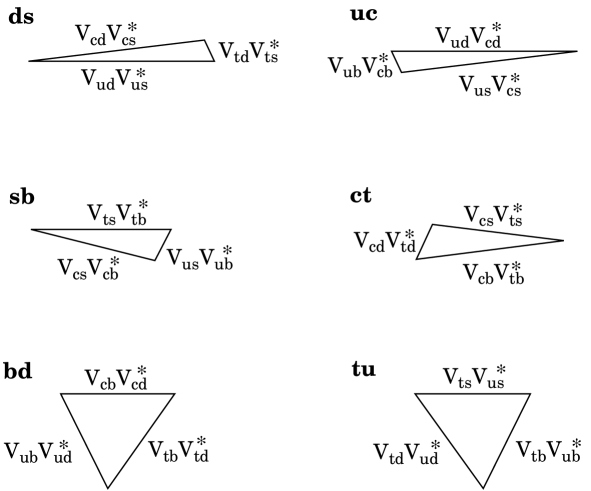
Рис. 3: Six unitarity triangles

2.4. The unitarity triangle

The unitarity of the CKM matrix implies various relations between its elements:

$$\sum\limits_{k}V_{ij}V_{kj}^{*}=\delta_{ij}$$ (19)

The unitarity triangles are geometrical representations in the complex plane of the six equations (19) with $i\neq k$. It is a trivial fact that any relationship of the form of a sum of three complex numbers equal to zero can be drawn as a closed triangle, see fig. 3.

All the unitarity triangles have the same area, $J/2$. However, while the triangles have the same area, they are of very different shapes: e.g. ds triangle has two sides of order $\lambda$ and one of order $\lambda^{4}$, while sb triangle has larger sides of order $\lambda^{2}$ and the small side of order $\lambda^{5}$ giving an angle of order $\lambda^{2}$. It would be very difficult to measure the area using such triangles. This leaves us with the bd triangle corresponding to the relation

$$V_{ud}^{*}V_{ub}+V_{cd}^{*}V_{cb}+V_{td}^{*}V_{tb}=0,$$ (20)

in which all sides are of order $\lambda^{3}$. The relation (20) is phenomenologically especially interesting as it involves simultaneously the elements $V_{ub}$, $V_{cb}$, and $V_{td}$, which are under extensive discussion at present. To an excellent accuracy $V_{cd}V_{cb}^{*}$ is

$$|V_{cd}V_{cb}^{*}|=A\lambda^{3}+{\cal O}(\lambda^{7})$$ (21)

Rescale all terms in (20) by $A\lambda^{3}$ and put the vector $V_{cd}V_{cb}^{*}$ on the real axis. The coordinates of the remaining vertex correspond to the $\rho$ and $\eta$ parameters or, in an improved version [18], to $\bar{\rho}=(1-\lambda^{2}/2)\rho$ and $\bar{\eta}=(1-\lambda^{2}/2)\eta$. The corresponding triangle is shown in Fig. 6.

The angles $\alpha$, $\beta$, and $\gamma$ (according to the BaBar collaboration, also known as, respectively, $\phi_{2}$, $\phi_{1}$, and $\phi_{3}$ according to the Belle collaboration) are defined as follows:

$$\alpha=arg\left(-\frac{V_{td}V_{tb}^{*}}{V_{ud}V_{ub}^{*}}\right),\leavevmode\nobreak\ \leavevmode\nobreak\ \beta=arg\left(-\frac{V_{cd}V_{cb}^{*}}{V_{td}V_{tb}^{*}}\right),\leavevmode\nobreak\ \leavevmode\nobreak\ \gamma=arg\left(-\frac{V_{ud}V_{ub}^{*}}{V_{cd}V_{cb}^{*}}\right).$$ (22)

The angles $\beta$ and $\gamma=\delta_{\rm CKM}$ of the unitarity triangle are related directly to the complex phases of the CKM-elements $V_{td}$ and $V_{ub}$, respectively, through

$$V_{td}=|V_{td}|e^{-i\beta},\quad V_{ub}=|V_{ub}|e^{-i\gamma}.$$ (23)

The lengths $R_{u}$ and $R_{t}$ are

$$R_{u}=|\rho+i\eta|=\left|\frac{V_{ud}V_{ub}^{*}}{V_{cd}V_{cb}^{*}}\right|,\leavevmode\nobreak\ \leavevmode\nobreak\ R_{t}=|1-\rho-i\eta|=\left|\frac{V_{td}V_{tb}^{*}}{V_{ud}V_{ub}^{*}}\right|.$$ (24)

Since the area of the unitarity triangle is $\eta/2$, a non-flat triangle implies $CP$ violation.

Within the SM the measurements of four CP conserving decays sensitive to $|V_{us}|$, $|V_{ub}|$, $|V_{cb}|$ and $|V_{td}|$ can tell us whether CP violation ($\bar{\eta}\not=0$) is predicted in the SM. This fact is often used to determine the angles of the unitarity triangle by measurements of $CP$ conserving quantities. The length of one side, $|\rho+i\eta|$, is extracted from a determination of $V_{ub}$, e.g from the rates of the forbidden $b\rightarrow u$ semileptonic transitions. CP-violating $K^{0}$–$\bar{K}^{0}$ mixing is dominated by $\bar{s}d\to\bar{d}s$ with virtual $t\bar{t}$ and $W^{+}W^{-}$ intermediate states. It constrains Im $(V_{td}^{2})\sim\bar{\eta}(1-\bar{\rho})$, giving a hyperbolic band in the $(\bar{\rho},\bar{\eta})$ plane. The important constraint comes from $B^{0}-\bar{B}{}^{0}$ mixing, which is mediated by the operator $\bar{b}\gamma^{\mu}(1-\gamma^{5})d\,\bar{b}\gamma^{\mu}(1-\gamma^{5})d$. In the SM, this operator is generated by the loop diagram for $\bar{b}d\to\bar{d}b$ (see Fig. 5), with a coefficient proportional to $|V_{td}{}^{*}V_{tb}|^{2}$. The phenomenological parameter $\Delta m_{d}$ is precisely measured, see subsection 3.1.. However, as in the case of $K^{0}-\bar{K}{}^{0}$ mixing, relating this number to fundamental quantities requires hadronic matrix elements which are difficult to compute.

The above mentioned determinations (schematically shown in Fig. 6) point to a non-flat triangle, i.e. to the presence of a certain amount of $CP$ violation.

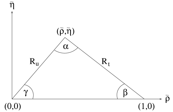
Рис. 4: Unitarity triangle corresponding to Eq. (20)

Рис. 5: SM box diagrams including $B^{0}-{\bar{B}}^{0}$ mixing.

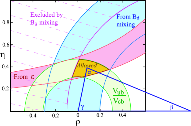
Рис. 6: Schematic determination of the unitarity triangle.

Several global analyses of the unitarity triangle have been performed, combining measurements of $|V_{cb}|$ and $|V_{ub}|$ in semileptonic $B$ decays, $|V_{td}|$ in $B$–$\bar{B}$ mixing, and the CP-violating phase of $V_{td}^{2}$ in $K$–$\bar{K}$ mixing and $B\to J/\psi\,K$ decays, see e.g. Refs. [20], [21]. The values obtained at 95% confidence level are

$$\bar{\rho}=0.178\pm 0.046,\leavevmode\nobreak\ \leavevmode\nobreak\ \bar{\eta}=0.341\pm 0.028.$$ (25)

The corresponding results for the angles of the unitarity triangle are

$$\sin 2\beta=0.705^{+0.042}_{-0.032},\leavevmode\nobreak\ \leavevmode\nobreak\ \leavevmode\nobreak\ \sin 2\alpha=-0.19\pm 0.25,\leavevmode\nobreak\ \leavevmode\nobreak\ \leavevmode\nobreak\ \gamma=(61.5\pm 7.0)^{\circ}.$$ (26)

These studies have established the existence of a CP-violating phase in the top sector of the CKM matrix, i.e., the fact that $\mbox{Im}(V_{td}^{2})\propto\bar{\eta}\neq 0$.

3. Express review of the phenomenology of CP violation

3.1. Time evolution and mixing

We first list the necessary formulae to describe $B^{0}-{\bar{B}}^{0}$ mixing. The formulae are general and apply to both $B_{d}^{0}$ and $B_{s}^{0}$ mesons although with different values of parameters. In the following, we use the standard convention that $B^{0}$ (${\bar{B}}^{0}$) contains $\bar{b}$ antidiquark ($b$ quark).

Once $CP$ is not a symmetry of the theory one must allow a more general form for the two mass eigenstates of neutral but flavored mesons. These two states are usually defined as $B_{H}$ and $B_{L}$ where the $H$ and $L$ stand for heavier and less heavy mesons. The light and heavy mass eigenstates can be written as linear combinations of $B^{0}$ and $\bar{B}^{0}$:

$$|B_{H}\rangle = p|{B^{0}}\rangle+q|{\bar{B}^{0}}\rangle,$$

$$|B_{L}\rangle = p|{B^{0}}\rangle-q|{\bar{B}^{0}}\rangle,$$ (27)

with

$$|q|^{2}+|p|^{2}=1.$$ (28)

The phase convention used here is $CP\leavevmode\nobreak\ |B^{0}>=|\bar{B}^{0}>$ that makes the phase of $q$ a meaningful quantity. The mass difference $\Delta m_{B}$ and the width difference $\Delta\Gamma_{B}$ are defined as follows:

$$\Delta m_{B}\equiv M_{H}-M_{L},\ \ \ \Delta\Gamma_{B}\equiv\Gamma_{H}-\Gamma_{L}.$$ (29)

The average mass and width are given by

$$m_{B}\equiv{M_{H}+M_{L}\over 2},\ \ \ \Gamma_{B}\equiv{\Gamma_{H}+\Gamma_{L}\over 2}.$$ (30)

The time evolution of the mass eigenstates is simple:

$$|B_{H}(t)\rangle = e^{-iM_{H}t}e^{-\Gamma_{H}t/2}|B_{H}(0)\rangle,$$

$$|B_{L}(t)\rangle = e^{-iM_{L}t}e^{-\Gamma_{L}t/2}|B_{L}(0)\rangle.$$ (31)

In the presence of flavor mixing the time evolution of $B^{0}$ and $\bar{B}^{0}$ is more complicated. An initially produced $B^{0}$ or ${\bar{B}}^{0}$ evolves in time into a superposition of $B^{0}$ and ${\bar{B}}^{0}$. Let $B^{0}(t)$ denotes the state vector of a $B$ meson which is tagged as $B^{0}$ at time $t=0$, i.e. $|B^{0}(t=0)>=B^{0}$. Likewise ${\bar{B}}^{0}(t)$ represent a $B$ meson initially tagged as ${\bar{B}}^{0}$. The time evolution of these states is governed by a Schrödinger-like equation

$$i{d\over dt}\pmatrix{B^{0}(t)\cr\bar{B}^{0}(t)\cr}=\left(M-{i\over 2}\Gamma\right)\pmatrix{B^{0}(t)\cr\bar{B}^{0}(t)\cr},$$ (32)

where the mass matrix $M$ and decay matrix $\Gamma$ are time independent, hermitian $2\times 2$ matrices written in the basis of the two flavor eigenstates. Both M and $\Gamma$ are complex with $M_{21}=M_{12}^{*}$, $\Gamma_{21}=\Gamma_{12}^{*}$ (hermicity), $M_{11}=M_{22}^{*}$, $\Gamma_{11}=\Gamma_{22}^{*}$ (CPT). $M_{12}$ is the dispersive part of the transition amplitude from $B^{0}$ to $\bar{B}^{0}$, while $\Gamma_{12}$ is the absorptive part of that amplitude. The off-diagonal terms in (32) are induced by $|\Delta B|=2$ transitions, so that the mass eigenstates of the neutral $B$ mesons that are defined as eigenvectors of $M-i\Gamma/2$ are different from the flavor eigenstates $B^{0}$ and ${\bar{B}}^{0}$. Solving the eigenvalue equation

$$\left(M-{i\over 2}\Gamma\right)\pmatrix{p\cr q\cr}=\lambda\pmatrix{p\cr q\cr},$$ (33)

we obtain

$$\lambda_{\pm}=M_{11}-\frac{i}{2}\Gamma_{11}\pm\sqrt{(M_{12}-\frac{i}{2}\Gamma_{12})(M_{12}^{*}-\frac{i}{2}\Gamma_{12}^{*})},$$ (34)

where $\lambda_{+}=\lambda_{H}$ and $\lambda_{-}=\lambda_{L}$. The off-diagonal (or mixing) elements are calculated from Feynman Diagrams that can convert one flavor eigenstate to the other. In the Standard Model these are dominated by the one loop box diagrams, shown in Fig. 5.

To find the time evolution of $B^{0}(t)$ and ${\bar{B}}^{0}(t)$ we invert Eqs. (3.1.) to express $B^{0}$ and ${\bar{B}}^{0}$ in terms of the mass eigenstates $B_{L}$ and $B_{H}$ and use their time evolution, Eqs. (3.1.). Then the evolution of the eigenstates (3.1.) of well-defined masses $M_{\pm}={\rm Re}(\lambda_{\pm})$ and decay widths $\Gamma_{\pm}=-2{\rm Im}(\lambda_{\pm})$ is given by the phases $\exp(-i\lambda_{\pm}t)$ where

$$\lambda_{\pm}=M_{\pm}-i\frac{1}{2}\Gamma_{\pm}t.$$ (35)

Using Eq. (34) one obtains

$$(\Delta m_{B})^{2}-{1\over 4}(\Delta\Gamma_{B})^{2}=(4|M_{12}|^{2}-|\Gamma_{12}|^{2}),\leavevmode\nobreak\ \leavevmode\nobreak\ \leavevmode\nobreak\ \Delta m_{B}\Delta\Gamma_{B}=4{\rm Re}(M_{12}\Gamma_{12}^{*}),$$ (36)

and

$${q\over p}=\sqrt{\frac{M_{12}^{*}-\frac{i}{2}\Gamma_{12}^{*}}{M_{12}-\frac{i}{2}\Gamma_{12}}}.$$ (37)

The time evolution of a pure $|B{{}^{0}}\rangle$ or $|\overline{B}{{}^{0}}\rangle$ state at $t=0$ is thus given by

$$|B{{}^{0}}(t)\rangle = g_{+}(t)\,|B{{}^{0}}\rangle+\frac{q}{p}\,g_{-}(t)\,|\overline{B}{{}^{0}}\rangle\,,$$ (38)

$$|\overline{B}{{}^{0}}(t)\rangle = g_{+}(t)\,|\overline{B}{{}^{0}}\rangle+\frac{p}{q}g_{-}(t)\,|B{{}^{0}}\rangle\,,$$ (39)

where

$$g_{\pm}(t)=\frac{1}{2}\left(e^{-i\lambda_{+}t}\pm e^{-i\lambda_{-}t}\right)\,.$$ (40)

The flavor states remain unchanged or oscillate into each other with time-dependent probabilities proportional to

$$\left|g_{\pm}(t)\right|^{2}=\frac{e^{-\Gamma_{B}t}}{2}\left[\cosh\!\left(\frac{\Delta\Gamma_{B}}{2}\,t\right)\pm\cos(\Delta m\,t)\right].$$ (41)

One can expect that $\Delta\Gamma_{B}/\Gamma_{B}\ll 1$ and $|\Gamma_{12}/M_{12}|\ll 1$ for $B^{0}-\bar{B}^{0}$ mixing (this is not the case for $K^{0}-\bar{K}^{0}$ mixing). The reason is that, on the one hand, it is experimentally known that $\Delta m_{B}/\Gamma_{B}\approx 0.7$. On the other hand, the difference in widths is produced by decay channels common to $B^{0}$ and $\bar{B}^{0}$. The branching ratios for such channels are at or below the level of $10^{-3}$. Since various channels contribute with differing signs, one expects that their sum does not exceed the individual level. Hence, we can safely assume that

$$\frac{\Delta\Gamma_{B}}{\Gamma_{B}}\sim\left|\frac{\Gamma_{12}}{M_{12}}\right|={\cal O}(10^{-2}).$$ (42)

To leading order in $|\Gamma_{12}/M_{12}|$, Eqs. (36) and (37) can be written as

$$\Delta m_{B}=2|M_{12}|,\leavevmode\nobreak\ \leavevmode\nobreak\ \leavevmode\nobreak\ \Delta\Gamma_{B}=2{\rm Re}\frac{M_{12}\Gamma_{12}^{*}}{|M_{12}|},$$ (43)

and

$$\frac{q}{p}=-\frac{M_{12}^{*}}{|M_{12}|}.$$ (44)

Note that the two mass eigenstates do not have to be orthogonal, in fact in general they will not be so, unless $|q/p|=1$.

3.2. The box diagram

The mass difference $\Delta m_{B}$ is is a measure of the oscillation frequency to change from $B^{0}$ to $\bar{B}^{0}$ and vise versa. Because the long distance contributions for $B^{0}-\bar{B}^{0}$ mixing are small (in contrast with the situation for $\Delta m_{K}$) $\Delta m_{B}$ and $\Delta m_{B}$ are very well approximated by the relevant box diagram. Since $m_{u,c}\ll m_{t}$ the only non-negligible contributions to $M_{12}$ and $\Gamma_{12}$ are from box diagrams involving two top quarks, the charm and mixed top-charm contributions are entirely negligible.

The dispersive ($M_{12}$) and absorptive ($\Gamma_{12}$) parts of top-mediated box diagrams are given by

$$M_{12}=-\frac{G_{F}^{2}m_{W}^{2}\eta_{B}m_{B}B_{B}f_{B}^{2}}{12\pi^{2}}\,S_{0}(\frac{m_{t}^{2}}{m_{W}^{2}})\,(V_{td}^{*}V_{tb})^{2},$$ (45)

$$\Gamma_{12}=\frac{G_{F}^{2}m_{b}^{2}\eta^{\prime}_{B}m_{B}B_{B}f_{B}^{2}}{8\pi}\,(V_{td}^{*}V_{tb})^{2},$$ (46)

where $m_{W}$ is the $W$ boson mass and $m_{i}$ is the mass of quark $i$. The factor $f_{B}$ is the vacuum-to-one-meson matrix element of the axial current, which arises in the naive approximation obtained by splitting the matrix element into two-quark terms and inserting the vacuum state between them. This is known as the vacuum-insertion approximation. The quantity $B_{B}$ is simply the correction factor between that approximate answer and the true answer. It can be estimated in various model calculations. The QCD corrections $\eta_{B}$ and $\eta^{\prime}_{B}$ are of order unity ($\eta_{B}=0.55\pm 0.01$). The known function $S_{0}(x_{t})$ can be approximated very well with

$$S_{0}(x_{t})=0.784\,x_{t}^{0.76}$$ (47)

For more details and further references see [19].

New physics usually takes place at a high energy scale and is relevant to the short distance part only. Therefore, the SM estimate in Eqs. (45) and (46) remains valid model independently. Combining (45) and (46), we obtain that

$$\left|\frac{\Gamma_{12}}{M_{12}}\right|\approx\frac{3\pi m_{b}^{2}}{2m_{W}^{2}S(x_{t})}\approx 5\times 10^{-3},$$ (48)

for $m_{b}=4.25$ GeV, $m_{W}=80$ GeV and $m_{t}=174$ GeV, which confirms our previous order of magnitude estimate. $2\phi_{B}=\arg(V_{td^{*}}V_{tb})^{2}$ is a CP violating phase. The phase of $\Gamma_{12}$ is given by

$$\arg\Gamma_{12}=2\phi_{B},$$ (49)

where $\phi_{B}$ is a CP violating phase:

$$2\phi_{b}=\arg(V_{td}^{*}V_{tb})^{2}=2\beta,$$ (50)

the phase of $M_{12}$ is

$$\arg M_{12}=2\beta+\pi.$$ (51)

The leading correction to this result is proportional to $(m_{c}/m_{b})^{2}$, more precisely, the phase difference between $M_{12}$ and $\Gamma_{12}$ is

$$\arg M_{12}-\arg\Gamma_{12}=\pi+\frac{8}{3}\left(\frac{m_{c}}{m_{b}}\right)^{2}\times\frac{\eta}{(1-\rho)^{2}+\eta^{2}},$$ (52)

i.e. i.e. $M_{12}$ and $\Gamma_{12}$ are almost antiparallel. For the $B$ system this leads to

$$\left(\frac{q}{p}\right)_{B}=e^{-2i\phi_{B}}.$$ (53)

At leading order in $\lambda$ and next-to-leading order in QCD, one finds

$$\Delta m_{B}=1.30\frac{G_{F}^{2}M_{W}^{2}}{6\pi^{2}}\cdot m_{B}\cdot f_{B}^{2}B_{B}\cdot A^{2}\lambda^{6}\cdot[(1-\rho)^{2}+\eta^{2}].$$ (54)

After surprising discovery of large $B^{0}-{\bar{B}}^{0}$ mixing by the Argus collaboration many $B^{0}-\bar{B}^{0}$ oscillations experiments were performed by the different experimental groups (for the complete list of references see [22]). Although a variety of techniques have been used, the individual $\Delta m_{B}$ results obtained at high-energy colliders have remarkably similar precision. Their average is compatible with the recent and more precise measurements from asymmetric $B$ factories. Before being combined, the measurements are adjusted on the basis of a common set of input values, including the $b$-hadron lifetimes and fractions. Combining all published measurements PDG 2002 quotes the value of

$$\Delta m_{B}={\rm 0.489\pm 0.005(stat)\pm 0.007(syst)}\leavevmode\nobreak\ \hbox{ps}^{-1}.$$ (55)

3.3. CP violating effects

.For the $B$ mesons it is useful to make a classification of CP-violating effects that is more transparent than the division into indirect and direct CP violation usually considered for the Kaon sector. In the SM, there are several possible ways of $CP$ violation. The first, seen for example in $K$ decays, occurs if $|q/p|\neq 1$. It is very clear in this case that no choice of phase conventions can make the two mass eigenstates be $CP$ eigenstates. This is generally called $CP$-violation in the mixing. A second possibility is $CP$ violation in the decay, or direct $CP$ violation, which requires that two $CP$-conjugate processes to have differing absolute values for their amplitudes. The third option is $CP$ violation in the interference between decays with and without mixing. We shall consider these cases step by step. A detailed presentation can be found e.g. in Ref. [8]

3.3.1 CP Violation in Mixing

This type of CP violation results from the mass eigenstates being different from the CP eigenstates, and requires a relative phase between $M_{12}$ and $\Gamma_{12}$, i.e. $|q/p|\neq 1$. CP violation in mixing has been observed in the neutral $K$ system (${\rm Re}\leavevmode\nobreak\ \varepsilon_{K}\neq 0$). For the neutral $B$ system, this effect can be best isolated by measuring the asymmetry in semileptonic decays:

$$A_{\rm SL}={\Gamma(\bar{B}^{0}(t)\to\ell^{+}\nu X)-\Gamma(B^{0}(t)\to\ell^{-}\nu X)\over\Gamma(\bar{B}^{0}(t)\to\ell^{+}\nu X)+\Gamma(B^{0}(t)\to\ell^{-}\nu X)}.$$ (56)

The final states in (56) contain ‘‘wrong charge’’ leptons and can be only reached in the presence of $B^{0}-{\bar{B}}^{0}$ mixing. As the phases in the $B^{0}-{\bar{B}}^{0}$ and ${\bar{B}}^{0}-B^{0}$ transitions differ from each other, a non-vanishing CP asymmetry follows. Specifically, for the time-integrated CP asymmetry one obtains

$$A_{\rm SL}={\rm Im}\leavevmode\nobreak\ \frac{\Gamma_{12}}{M_{12}}\approx-1.4\times 10^{-3}{\eta\over(1-\rho)^{2}+\eta^{2}}.$$ (57)

The suppression by a factor of ${\cal O}(10)$ of $a_{\rm SL}$ compared to $|\Gamma_{12}/M_{12}|$ comes from the fact that the leading contribution to $\Gamma_{12}$ has the same phase as $M_{12}$. Consequently, $A_{\rm SL}={\cal O}(m_{c}^{2}/m_{t}^{2})$. The CKM factor does not give any further significant suppression,

$${\rm Im}\frac{V_{cb}V_{cd}^{*}}{V_{tb}V_{td}^{*}}={\cal O}(1).$$ (58)

In contrast, for the $B_{s}$ system, where the same expressions holds except that $V_{cd}/V_{td}$ is replaced by $V_{cs}/V_{ts}$, there is an additional CKM suppression from

$${\rm Im}\frac{V_{cb}V_{cs}^{*}}{V_{tb}V_{ts}^{*}}={\cal O}(\lambda^{2}).$$ (59)

To estimate $A_{\rm SL}$ in a given model, one needs to calculate $M_{12}$ and $\Gamma_{12}$. This involves some hadronic uncertainties, in particular in the hadronization models for $\Gamma_{12}$.

The asymmetry $A_{SL}$ has been searched for in several experiments, with sensitivity at the level of $10^{-2}$ giving a world average of

$$A_{\rm SL}=(0.2\pm 1.4)\times 10^{-2}.$$ (60)

3.3.2 CP violation in decay

We define the decay amplitudes $A_{f}$ and $\bar{A}_{f}$ according to

$$A_{f}=\langle f|{\cal H}_{d}|B^{0}\rangle,\ \ \ \bar{A}_{f}=\langle f|{\cal H}_{d}|\bar{B}^{0}\rangle,$$ (61)

where ${\cal H}_{d}$ is the decay Hamiltonian.

CP relates $A_{f}$ and $\bar{A}_{\bar{f}}$. There are two types of phases that may appear in $A_{f}$ and $\bar{A}_{\bar{f}}$. Complex parameters in any Lagrangian term that contributes to the amplitude will appear in complex conjugate form in the CP-conjugate amplitude. Thus their phases appear in $A_{f}$ and $\bar{A}_{\bar{f}}$ with opposite signs. In the SM, these phases occur only in the mixing matrices , hence these are often called ‘‘weak phases’’. The weak phase of any single term in $A_{f}$ is convention dependent. However the difference between the weak phases in two different terms in $A_{f}$ is convention independent because the phase rotations of the initial and final states are the same for every term. A second type of phase can appear in scattering or decay amplitudes even when the Lagrangian is real. Such phases do not violate CP and they appear in $A_{f}$ and $\bar{A}_{\bar{f}}$ with the same sign. Their origin is the possible contributions from coupled channels. Usually the dominant re scattering is due to strong interactions and hence the designation ‘‘strong phases’’ for the phase shifts so induced. Again only the relative strong phases of different terms in a scattering amplitude have physical content, an overall phase rotation of the entire amplitude has no physical consequences. Thus it is useful to write each contribution to $A$ in three parts: its magnitude $A_{i}$; its weak phase term $e^{i\phi_{i}}$; and its strong phase term $e^{i\delta_{i}}$. Then, if several amplitudes contribute to $B\to f$, we have

$$\left|{\bar{A}_{\bar{f}}\over A_{f}}\right|=\left|{\sum_{i}A_{i}e^{i(\delta_{i}-\phi_{i})}\over\sum_{i}A_{i}e^{i(\delta_{i}+\phi_{i})}}\right|.$$ (62)

3.3.3 CP violation in the interference of decays with and without mixing

One can learn CKM phases from decays of neutral $B$ mesons to CP eigenstates $f_{CP}$. As a result of $B^{0}-\bar{B}^{0}$ mixing, a state which is $B^{0}$ at proper time $t=0$ will evolve into one, denoted $B^{0}(t)$, which is a mixture of $B^{0}$ and $\bar{B}^{0}$. Thus there will be one pathway the final state $f_{CP}$ from $B^{0}$ throughout the amplitude $A_{f_{CP}}$ and another from $\bar{B}^{0}$ through the amplitude $\bar{A}_{f_{CP}}$, which acquires an additional phase $2\beta$ trough the mixing. The CP invariance is violated when the time-dependent decay rate of $B^{0}\to f_{CP}$ and that of the CP conjugated decay $\bar{B}^{0}\to f_{CP}$ are different:

$$\Gamma_{B^{0}\to f_{CP}}(t)\neq\Gamma_{B^{0}\to f_{CP}}(t)$$ (63)

for any $t$.

The interference of the amplitudes $A_{f_{CP}}$ and $\bar{A}_{f_{CP}}$ can differ in the decays $B^{0}(t)$ and $\bar{B}^{0}(t)$ leading to a time dependent asymmetry. To calculate this asymmetry it is convenient to introduce a complex quantity $\lambda_{f}$ defined by

$$\lambda_{CP}=\left(\frac{q}{p}\right)_{B}\frac{\bar{A}_{f_{CP}}}{A_{f_{CP}}}=e^{-2i\beta}\frac{\bar{A}_{f_{CP}}}{A_{f_{CP}}}.$$ (64)

In the case $\Delta\Gamma_{B}\ll\Gamma$ one obtains for time dependent rates

$$\left\{\begin{array}[]{c}\Gamma[B^{0}(t)\to f]\\ \Gamma[\bar{B}^{0}(t)\to f]\end{array}\right\}\sim e^{-\Gamma t}[1\mp{\cal A}_{CP}\cos\Delta m_{B}t\mp{\cal S}_{CP}\sin\Delta m_{B}t]\leavevmode\nobreak\ \leavevmode\nobreak\ \leavevmode\nobreak\ ,$$ (65)

where

$${\cal A}_{CP}\equiv\frac{|\lambda_{CP}|^{2}-1}{|\lambda_{CP}|^{2}+1}\leavevmode\nobreak\ \leavevmode\nobreak\ ,\leavevmode\nobreak\ \leavevmode\nobreak\ \leavevmode\nobreak\ {\cal S}_{CP}\equiv\frac{2{\rm Im}\lambda_{CP}}{|\lambda_{CP}|^{2}+1}\leavevmode\nobreak\ \leavevmode\nobreak\ ,$$ (66)

where $A\,(\bar{A})$ denotes the $B^{0}\,(\bar{B}^{0})\to f_{\rm CP}$ decay amplitude. Note that ${\cal S}_{f}^{2}+{\cal A}_{f}^{2}\leq 1$.

The weak phase $\phi_{f}$ is the phase of $A_{f}$. Therefore

$$\frac{\bar{A}_{f}}{A_{f}}=e^{-2i\phi_{f}}.$$ (67)

Eqs. (53) and (67) together imply that for a final CP eigenstate,

$$\lambda_{f_{\rm CP}}=\eta_{f_{\rm CP}}e^{-2i(\phi_{B}+\phi_{f})},$$ (68)

where $\eta_{f_{\rm CP}}=\pm 1$ is the CP eigenvalue of the final state.

To illustrate the phase structure of decay amplitudes, consider the process in which the $\bar{b}$-quark decays through $\bar{b}\to{\it q}\bar{\it q}{\it d}$ decay, where $q$ is an up-quark ($u$ or $c$), ${\it d}$ is the corresponding down quark. The decay Hamiltonian is of the form

$$H_{d}\propto e^{+i\phi_{f}}[\bar{\it q}\gamma^{\mu}(1-\gamma_{5}){\bar{\it d}}][\bar{b}\gamma_{\mu}(1-\gamma_{5}){\it q}]+e^{-i\phi_{f}}[\bar{\it q}\gamma^{\mu}(1-\gamma_{5})b][\bar{\it d}\gamma_{\mu}(1-\gamma_{5}){\it u}].$$ (69)

In this case

$$\frac{\bar{A}_{f}}{A_{f}}=\frac{V_{{\it q}b}V_{{\it qd}}^{*}}{V_{{\it q}b}^{*}V_{\it qd}}.$$ (70)

We now consider two specific examples.

3.4. $B\to J/\psi K_{S}$. $\sin 2\beta$ measurements

The parameter $\sin 2\beta$ is directly accessible through a study of $CP$ violation in the ‘‘golden decay mode’’ of $B^{0}$ mesons

$$B^{0}\leavevmode\nobreak\ {\rm or}\leavevmode\nobreak\ \bar{B}^{0}\rightarrow J/\psi K_{S}.$$ (71)

The ‘‘golden’’ character of $B^{0}\rightarrow J/\psi K_{S}$ derives from the fact that the final state is a $CP$ eigenstate, and that this decay mode is dominated by a $CP$ conserving tree diagram. Any $CP$ violation observed in this mode must, to an excellent approximation, be attributed to $B^{0}-\bar{B}^{0}$ mixing. The transitions $B^{0}-\bar{B}^{0}$ are described, in the lowest order, by a single box diagram involving two $W$ bosons and two $up$-type quarks. The phase of the box diagram was seen to be $\exp(2\,i\,\beta)$. Therefore measurement of $CP$ violation effects in this decay mode can be directly interpreted as a measurement of the $\beta$ angle in the unitarity triangle.

As it was discussed in the preceding subsections, in decays of neutral $B$ mesons into a CP eigenstate $f_{\rm CP}$, an observable CP asymmetry can arise from the interference of the amplitudes for decays with an without $B$–$\bar{B}$ mixing, i.e., from the fact that the amplitudes for $B^{0}\to f_{\rm CP}$ and $B^{0}\to\bar{B}^{0}\to f_{\rm CP}$ must be added coherently. For the time dependent asymmetry one obtains from Eqs. (65), (66)

$$A_{\rm CP}(t) = \frac{\Gamma(\bar{B}^{0}(t)\!\to\!f_{\rm CP})-\Gamma(B^{0}(t)\!\to\!f_{\rm CP})}{\Gamma(\bar{B}^{0}(t)\!\to\!f_{\rm CP})+\Gamma(B^{0}(t)\!\to\!f_{\rm CP})}=$$ (72)

$$\frac{2\mbox{Im}(\lambda_{CP})}{1+|\lambda_{C}P|^{2}}\sin(\Delta m_{B}t)-\frac{1-|\lambda_{CP}|^{2}}{1+|\lambda_{CP}|^{2}}\cos(\Delta m_{B}t),$$

where $\phi_{B}$ is the introduced above $B$–$\bar{B}$ mixing phase (which in the SM equals $-2\beta$).

Рис. 7: Tree and penguin topologies in $B\to J/\psi\,K$ decays.

The decay is mediated by the quark transition $\bar{b}\to\bar{c}c\bar{s}$. In the SM, the this decay can proceed via tree level diagram or via penguin diagrams with intermediate $u$, $c$ and $t$ quarks, as shown in Figure 7. The tree diagram has a CKM factor $V_{cb}^{*}V_{cs}$. An amplitude P of penguin diagram has three terms, corresponding to the three different up-type quarks inside the loop and can be written in the following schematic form

$$P=V_{tb}^{*}V_{ts}f(m_{t})+V_{cb}^{*}V_{cs}f(m_{c})+V_{ub}^{*}V_{us}f(m_{u}),$$ (73)

where the $f(m_{q})$ is some function of the quark mass. We use the unitarity relationship to rewrite the three terms in (73) in terms of two independent CKM factors:

$$P=V_{cb}^{*}V_{cs}[f(m_{c})-f(m_{t})]+V_{ub}^{*}V_{us}[f(m_{u})-f(m_{t})].$$ (74)

The first of these is the same as that for the tree term, so for the present discussion it can be considered as part of the ‘‘tree amplitude’’. The second term is suppressed by two factors. First, ignoring CKM factors, the penguin graph contribution is expected to be suppressed compared to the tree graph, because it is a loop graph and has an additional hard gluon. Second, it is CKM suppressed by an additional factor of

$$\left|\frac{V_{ub}^{*}V_{us}}{V_{cb}^{*}V_{cs}}\right|\sim\lambda^{2}.$$ (75)

The ‘‘penguin pollution’’ to the weak phase is of order

$$\phi_{A}\sim\lambda^{2}\left|\frac{P}{T}\right|\sim 1\%,$$ (76)

where $|P/T|\sim 0.2$ is the tree-to-penguin ratio.

Thus we have an amplitude that effectively has only a single CKM coefficient and hence one overall weak phase, which means there is no decay-type (direct) $CP$ violation. Indeed, we need at least two terms with different weak phases to get such an effect. This then ensures

$$\frac{\bar{A}_{J/\psi K_{S}}}{A_{J/\psi K_{S}}}=\left(\frac{V_{cb}V_{cs}^{*}}{V_{cb}^{*}V_{cs}}\right)\left(\frac{V_{cs}V_{cd}^{*}}{V_{cs}^{*}V_{cd}}\right).$$ (77)

The last factor is $(q/p)_{K}$ in $K^{0}-\bar{K}^{0}$ mixing. This is crucial because in the absence of $K^{0}-\bar{K}^{0}$ mixing there could be no interference between ${\bar{B}}^{0}\to J/\psi{\bar{K}}^{0}$ and $B^{0}\to J/\psi K^{0}$. Then one finds

$$\hat{\lambda}_{J/\psi K_{S}}=-\left(\frac{V_{tb}^{*}V_{td}}{V_{tb}V_{td^{*}}}\right)\left(\frac{V_{cb}V_{cs}^{*}}{V_{cb}^{*}V_{cs}}\right)\left(\frac{V_{cs}V_{cd}^{*}}{V_{cs}^{*}V_{cd}}\right)=-\exp(-2i\beta),$$ (78)

where the first factor is the SM value for the $(q/p)_{B}$ in $B^{0}-\bar{B}^{0}$ mixing. Recall that for the $B$ meson we expect $|q/p|_{B}=1$ to a good approximation. Thus $A_{J/\psi K_{S}}$ measures Im$\leavevmode\nobreak\ \lambda_{J/\psi K_{S}}=\sin 2\beta$:

$$A_{CP}(t)\simeq\sin 2\beta\sin(\Delta m_{B}t).$$ (79)

The results (1) obtained by Belle experiment and by Babar experiment are in reasonable agreement among themselves. Combining Belle and BaBar results with earlier measurements by CDF at Fermilab $(0.79^{+0.41}_{-0.44})$, ALEPH and OPAL at CERN $(0.84^{+0.82}_{-1.04}\pm 0.16)$ gives the ‘‘world average’’

$$\sin 2\beta=0.734\pm 0.054\leavevmode\nobreak\ .$$ (80)

3.5. $B\to\pi^{+}\pi^{-}$. $\sin 2\alpha$ measurements

To measure the angle $\alpha$, the most promising and straightforward approach involves the use of the decay mode $B^{0}\to\pi^{+}\pi^{-}$ which is an example of the final CP eigenstate. The interference in this mode between direct decay and the decay via mixing leads to a CP violating asymmetry as in the charmonium mode $B^{0}\to J/\psi K_{S}.$

However there are several additional complications. The decay amplitude for $B^{0}\to\pi^{+}\pi^{-}$ contains a contribution from a tree diagram ($\bar{b}\to\bar{u}ud$) as well as Cabbibo suppressed penguin diagram which has the flavor structure $\bar{b}\to\bar{d}$ with the final $\bar{d}d$ pair fragmenting into $\pi^{+}\pi^{-}$. The magnitude of the tree amplitude is $|T|$; its weak phase is Arg($V^{*}_{ub})=\gamma$; by convention its strong phase is 0. The amplitude of the penguin amplitude is $|P|$. The dominant $t$ contribution in the loop diagram for $\bar{b}\to\bar{d}$ can be integrated out and the unitarity relation $V_{td}V^{*}_{tb}=-V_{cd}V^{*}_{cb}-V_{ud}V^{*}_{ub}$ used. The $V_{ud}V^{*}_{ub}$ contribution can be absorbed into a redefinition of the tree amplitude. By definition, its strong phase is $\delta$. However the remaining penguin contributions are not negligible (as in the previous case $B^{0}\to J/\psi K_{S}$) and has a weak phase that is different from the phase of the tree amplitude, which is zero in the usual parameterization. Therefore the time dependent asymmetry, proportional to $\sin\Delta m_{B}$, which is measured is not equal to $\sin 2\alpha$ but instead will have a large unknown correction. The presence of the extra contribution also induces an additional time dependent term proportional to $\cos\Delta m_{B}t$.

The time-dependent asymmetries $S_{\pi\pi}$ and $A_{\pi\pi}$ specify both $\alpha$ and $\delta$, if one has an independent estimate of $|P/T|$. One may obtain $|P|$ from $B^{+}\to K^{0}\pi^{+}$ using flavor SU(3) [23] and $|T|$ from $B\to\pi l\nu$ using factorization [24]. An alternative method [25] uses the measured ratio of the $B^{+}\to K^{0}\pi^{+}$ and $B^{0}\to\pi^{+}\pi^{-}$ branching ratios to constrain $|P/T|$. The update value of $|P/T|$ is $0.28\pm 0.06$ [26].

Таблица 2: Values of $S_{\pi\pi}$ and $A_{\pi\pi}$ quoted by BaBar and Belle. The errors for average $S_{\pi\pi}$ and $A_{\pi\pi}$ are taken from [26]

	BaBar [27]	Belle [28]	Average
$S_{\pi\pi}$	$0.02\pm 0.34\pm 0.05$	$-1.23\pm 0.41^{+0.08}_{-0.07}$	$-0.49\pm 0.61$
$A_{\pi\pi}$	$0.30\pm 0.25\pm 0.04$	$0.77\pm 0.27\pm 0.08$	$\leavevmode\nobreak\ \leavevmode\nobreak\ 0.51\pm 0.23$

The experimental situation regarding the time dependent asymmetries is not yet settled. As shown in Table 2, BaBar and Belle obtain different asymmetries, especially $S_{\pi\pi}$. At present values of $\alpha\leavevmode\nobreak\ >90^{\circ}$ are favorated, but with large uncertainty. It is not yet settled whether ${\cal A}_{\pi\pi}\neq 0$, corresponding to ‘‘direct’’ CP violation.

3.6. Conclusions

The significance of the $\sin 2\beta$ measurements is that for the first time a large CP asymmetry has been observed, proving that CP is not an approximate symmetry of Nature. Rather, the CKM phase is, very likely, the dominant source of CP violation in low-energy flavor-changing processes. This opens a new era, in which the model is expected to be scrutinized through a variety of other $B$ and $B_{s}$ decay asymmetries. Impressive progress has already been made in search for asymmetries in several hadronic $B$ decays, including $B^{0}\to\pi^{+}\pi^{-}$, $B^{0,\pm}\to K\pi$ and $B^{\pm}\to DK^{\pm}$. Current measurements are approaching the level of tightening bounds on the CP-violating phase $\gamma$. These and forthcoming measurements of $B_{s}$ decays will enable a cross-check of the CKM model.

4. $V_{cb}$ determination

As discussed in Section 2, $|V_{cb}|$ sets the overall scale for the lengths of the sides, and $|V_{ub}|$ determines the length of one side. Precise determinations of both are needed to complement the measurement of the angles of the unitarity triangle. In this section we shall discuss exclusive semileptonic decays of $B$-mesons, in which the $b$-quark decays into a $c$-quark, and from which one can determine the $|V_{cb}|$ elements of the CKM-matrix. In principle, $|V_{cb}|$ can be studied in any weak decay mediated by the W boson. Semileptonic decays offer the advantage that the leptonic current is calculable and QCD complications only arise in the hadronic current. Unlike hadronic decays, there are no final state interactions. One still needs some understanding of the strong interaction. Some approaches offer detailed predictions for the QCD dynamics in heavy quark decays. These predictions allow measurement of $|V_{cb}|$ with reasonable precision.

4.1. $\rm B\to D^{\star}\ell\nu$ and $\rm B\to D\ell\nu$ decays

The exclusive $|V_{cb}|$ determination is obtained studying the $\rm B\to D^{\star}\ell\nu$ and $\rm B\to D\ell\nu$ decays. These decays have been studied in experiments performed at the $\Upsilon(4S)$ center of mass energy (CLEO [29] , Belle [30]) and at the $Z^{0}$ center of mass energy at LEP (ALEPH [31], DELPHI [32], and OPAL [33]).

4.1.1 Kinematics

The hadronic form factors for semileptonic decays are defined as the Lorentz–invariant functions arising in the covariant decomposition of matrix elements of the vector and axial currents. It is conventional to parameterize these matrix elements by a set of scalar form factors. The most appropriate to the heavy-quark limit is the set of form factors $h_{i}(w)$, which are defined separately for the vector and axial currents:

$$\langle D(v^{\prime})|\,\bar{c}\gamma^{\mu}b\,|B(v)\rangle=h_{+}(w)(v+v^{\prime})^{\mu}+h_{-}(w)(v-v^{\prime})^{\mu},$$ (81)

$$\langle D(v^{\prime})|\,\bar{c}\gamma^{\mu}\gamma^{5}b\,|B(v)\rangle=0,$$ (82)

$$\langle D^{*}(v^{\prime},\epsilon)|\,\bar{c}\gamma^{\mu}b\,|B(v)\rangle=h_{V}(w)i\varepsilon^{\mu\nu\alpha\beta}\epsilon_{\nu}^{*}v^{\prime}_{\alpha}v_{\beta},$$ (83)

$$\langle D(v^{\prime})|\,\bar{c}\gamma^{\mu}\gamma^{5}b\,|B(v)\rangle=h_{A_{1}}(w)(w+1)\epsilon^{*\mu}-\epsilon^{*}\cdot v[h_{A_{2}}(w)v^{\mu}+h_{A_{3}}(w)v^{\prime\mu}]\,$$ (84)

where meson states are denoted as $|P(v)>$ for a pseudoscalar state and $|V(v,\varepsilon>)$ for a vector state, where $v$ is the 4-velocity of a state and $\varepsilon$ is the polarization vector, $w=v\cdot v^{\prime}$ is the velocity transfer which is linearly related to $q^{2}$, the invariant mass of the $W$. Other linear combinations of form factors are also used in the literature, see e.g. [34]

In the case of heavy–to–heavy transitions, in the limit in which the active quarks have infinite mass, all the form factors are given in terms of a single function ${\cal F}(w)$, the Isgur–Wise form factor [35]:

$$h_{+}(w)=h_{V}(w)=h_{A_{1}}(w)=h_{A_{3}}(w)={\cal F}(w),$$

$$h_{-}(w)=h_{A_{2}}(w)=0.$$ (85)

In the realistic case of finite quark masses these relations are modified: each form factor depends separately on the dynamics of the process.

4.1.2 The decay $\rm B\to D^{*}\ell\nu$ in Heavy Quark Effective Theory

Heavy Quark Effective Theory (HQET), see e.g. [36], predicts that the differential partial decay width for $B\rightarrow D^{\star}\ell\nu$, $d\Gamma/dw$, is related to $V_{cb}$ through:

$$\frac{d\Gamma}{dw}(B\rightarrow D^{\star}\ell\nu)=\frac{G_{F}^{2}|V_{cb}|^{2}}{48\pi^{3}}{\cal K}(w){\cal F}_{D^{*}}^{2}(w),$$ (86)

where ${\cal K}(w)$ is a known phase space factor:

$${\cal K}(w)=(m_{B}{-}m_{D^{*}})^{2}m_{D^{*}}^{3}\sqrt{w^{2}{-}1}\,(w{+}1)^{2}\left[1+\frac{4w}{w{+}1}\frac{m_{B}^{2}-2wm_{B}m_{D^{*}}+m_{D^{*}}^{2}}{(m_{B}-m_{D^{*}})^{2}}\right].$$ (87)

The function ${\cal F}_{D^{*}}(w)$ is the form factor for the $B$ to $D^{*}$ transition, i.e., the Isgur-Weise function combined with perturbative and power corrections. The precision with which $V_{cb}$ can be extracted is limited by the theoretical uncertainties in the evaluation of these corrections.

In the infinite quark mass limit in the kinematical point where $D^{*}$ is at rest in the $B$ rest frame the wave function overlap is 1, i.e., ${\cal F}_{D^{*}}=1$. There are several different corrections to the infinite mass value ${\cal F}_{D^{*}}(1)=1$:

$${\cal F}_{D^{*}}(1)=\eta_{QED}\eta_{A}\left[1+\delta_{1/m_{Q}^{2}}+...\right],\leavevmode\nobreak\ \leavevmode\nobreak\ \leavevmode\nobreak\ Q=c,b$$ (88)

The correction ${\cal O}(1/m_{Q})$ vanishes by virtue of Luke’s theorem [37]. $QED$ corrections $\eta_{QED}\approx 1.007$ up to leading logarithms. $QCD$ radiative corrections to two loops give $\eta_{A}=0.960\pm 0.007$. Different estimates of the $1/m_{Q}^{2}$ corrections yield

$$1+\delta_{1/m_{Q}^{2}}=\ 0.91\pm 0.04$$ (89)

The analytical expression of ${\cal F}_{D^{*}}(w)$ is not known a-priori, and this introduces an additional uncertainty in the determination of ${\cal F}_{D^{*}}(1)|V_{cb}|$. In an experiment one measures the decay rate as function of $w$ and extrapolates to $w=1$. As the kinematically allowed range of $w$ is small ($w\in[1.0,1.5]$), the form factor is approximated as a Taylor expansion around $w=1$.

$${\cal F}_{D^{*}}(w)={\cal F}_{D^{*}}(1)(1+(w-1)\rho^{2}+c(w-1)^{2}).$$ (90)

Fig. 8 shows the latest CLEO measurement [29] of ${\cal F}_{D^{*}}|V_{cb}|$ as a function of $w$. The results of the fits of the latest experiments are given in Tabl. 3. Averaging the data one gets

$${\cal F}_{D^{*}}(1)|V_{cb}|=(38.3\pm 1.0)\times 10^{-3}.$$ (91)

This gives the most updated value quoted from [10]

$$|V_{cb}|=(42.1\pm 1.1_{exp}\pm 1.9_{theo})\times 10^{-3}.$$ (92)

Experiment	$|V_{cb}|\times 10^{3}$	$\rho^{2}$
CLEO [29]	43.3$\pm$ 1.3$\pm$ 1.8	1.61$\pm$ 0.09$\pm$ 0.21
Belle [30]	36.0$\pm$ 1.9$\pm$ 1.8	1.45$\pm$ 0.16$\pm$ 0.20
ALEPH [31]	33.8$\pm$ 2.1$\pm$ 1.6	0.74$\pm$ 0.25$\pm$ 0.41
DELPHI [32]	36.1$\pm$ 1.4$\pm$ 2.5	1.42$\pm$ 0.14$\pm$ 0.37
OPAL [33]	38.5$\pm$ 0.9$\pm$ 1.8	1.35$\pm$ 0.12$\pm$ 0.31

Таблица 3: Various experimental results for $|V_{cb}|$. For details see [10]. $\rho^{2}$ is the slope of the form factor at zero recoil as defined in (90).

4.2. $B\to D\ell\nu$

The decay $B\to D\ell\nu$ can be analyzed in the same way as $B\to D^{*}\ell\nu$ decay. The differential decay width for $B\to D\ell\nu$ decay is

$${d\Gamma\over dw}={G_{F}^{2}|V_{cb}|^{2}\over 48\pi^{3}}(M_{B}+M_{D})^{2}M_{D}^{3}(w^{2}-1)^{3/2}{\cal F}_{D}^{2}(w)$$ (93)

where different form factor ${\cal F}_{D}(w)$ is assumed. The precision with which $|V_{cb}|$ can be determined is not as good as for $B\to D^{*}\ell\nu$ because of smaller branching fraction, larger backgrounds and an additional kinematic suppression factor $w^{2}-1$ (compare Eqs. (86) and (93)). Nonetheless it provides complementary information and provides a test of HQET predictions for the relationships between the form factors for semileptonic decays $B\to D$ and $B\to D^{*}$.

Theoretical predictions for ${\cal F}_{D}(1)$ are: $1.03\pm 0.07$ (quark model [38]) and $0.98\pm 0.7$ (QCD sum rules [39]). A quenched lattice calculation gives ${\cal F}(1)=1.058^{+0.020}_{-0.017}$ [40]. Using ${\cal F}_{D}(1)=1.0\pm 0.07$ PDG 2002 quotes the value

$$|V_{cb}|=(41.3\pm 4.0_{exp}\pm 2.9_{theo})\times 10^{-3},$$ (94)

consistent with (92).

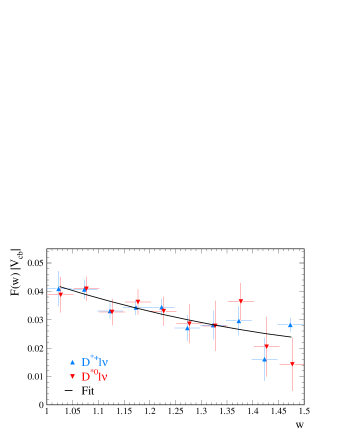
Рис. 8: Overlay of ${\cal F}_{D^{*}}(w)|V_{cb}|$ where the points are $B\to D^{*}\ell\nu$ data

4.3. Inclusive semileptonic decays

Alternatively, $|V_{cb}|$ can be extracted from measuring of electron energy spectra in inclusive semileptonic $B\to X_{c}\ell\nu$ decay . Inclusive measurements are employed to avoid the need for form factors, relying on HQET for the necessary quark level input.

The measurement [41] employs the method introduced by ARGUS [42] and later used by CLEO [43], in which $B\bar{B}$ events are tagged by the presence of a high momentum lepton. As a tag, electrons are chosed with center-of-mass frame momentum $1.4GeV/c\leavevmode\nobreak\ <p^{*}<\leavevmode\nobreak\ 2.3GeV/c$. A second electron in the event is taken as the signal lepton for which the condition $p^{*}>p_{min}$ is required to avoid large backgrounds at lower momenta. Signal electrons are mostly from primary B decays if they are accompanied by a tag electron of opposite charge (unlike-sign). Those with a tag of the same charge (like-sign) originate predominantly from secondary decays of charm particles produced in the decay of the other B meson. Inversion of this charge correlation due to $B^{0}\bar{B}^{0}$ mixing is treated explicitly, and unlike-sign pairs with both electrons originating from the same B meson are isolated kinematically. With a small model-dependence on the estimated fraction of primary electrons below $p^{*}=0.6$ GeV/c, the semileptonic B branching fraction is inferred from the background corrected ratio of unlike-sign electron pairs to tag electrons.

The $B\to X_{c}e\nu$ electron spectrum measurement [43] shown in Fig. 9 is an observed spectrum above 0.6 GeV. In events with a high momentum lepton tag and an additional electron, the primary electrons ($b\to c\ell^{-}X$) are separated from secondary electrons from charm decays ($b\to cX;c\to\ell^{+}Y$ ) using angular and charge correlations.

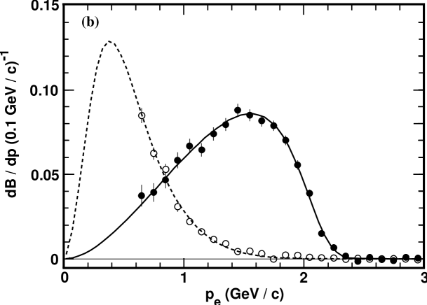
Рис. 9: Electron momentum spectrum from $B\to X_{e}\nu$ (solid circles) and $b\to c\to Ye\nu$ (open circles) [43]. The curves show the best fit to the ISGW model with 23% $B\to D^{**}\ell\nu$.

For beauty hadrons with $m_{b}\gg\Lambda_{QCD}$ or $\bar{\Lambda}$, a QCD related scale of order 400 MeV (see below), one can use an operator product expansion (OPE) [44] combined with HQET. The spectator model decay rate is the leading term in a OPE expansion controlled by the parameter $\bar{\Lambda}/m_{b}$. Non-perturbative corrections to the leading approximation arise only to order $1/m_{b}^{2}$. The key issue in this approach is the ability to separate non-perturbative corrections, which can be expressed as a series in powers of $1/m_{b}$, and perturbative corrections, expressed in powers of $\alpha_{s}$. Quark-hadron duality is an important ab initio assumption in these calculations [45]. An unknown correction may be associated with this assumption. Arguments supporting a possible sizeable source of errors related to the assumption of quark-hadron duality have been proposed [46]. This issue needs to be resolved with further measurements.

The OPE result for inclusive decay width $\Gamma_{SL}$ reads

$$\Gamma_{SL} = \frac{G_{F}^{2}m_{b}^{5}}{192\pi^{3}}\cdot\left(1-a_{1}\frac{\alpha_{s}}{\pi}-a_{2}(\frac{\alpha_{s}}{\pi})^{2}+...\right)$$ (95)

$$\times\left((1+\frac{\lambda_{1}}{2m_{b}^{2}})f(\rho)+\frac{\lambda_{2}}{2m_{b}^{2}}g(\rho)\leavevmode\nobreak\ +\leavevmode\nobreak\ ...\right),$$

where $a_{1}=1.54,\leavevmode\nobreak\ a_{2}=1.43\beta_{0}$ ($\beta_{0}$ being the $\beta$ function) are coefficients of the perturbative expansion, $m_{b}(\mu)$ and $m_{c}(\mu)$ are short scale quark masses (in particular, $\rm m_{b}(\mu\sim 1\leavevmode\nobreak\ \rm GeV)=4.58\pm 0.09\ GeV$), $f(\rho)$ and $g(\rho)$ are known parton phase space factors,

$$f(\rho)=1-8\rho+8\rho^{3}-\rho^{4}-12\rho^{2}\log\leavevmode\nobreak\ \rho,$$ (96)

$$g(\rho)=-9+24\rho-72\rho^{2}+72\rho^{3}-15\rho^{4}-36\rho^{2}\log\leavevmode\nobreak\ \rho,$$ (97)

with $\rho=m_{c}^{2}/m_{b}^{2}$.

The parameters $\lambda_{1}$ and $\lambda_{2}$ are matrix elements of the HQET expansion, which have the following intuitive interpretations: $\lambda_{1}$ is proportional to the kinetic energy of the $b$-quark in the $B$ meson and $\lambda_{2}$ is the energy of the hyperfine interaction of the $b$-quark spin and the light degrees of freedom in the meson. The third HQET parameter, $\bar{\Lambda}$, representing the energy of the light degrees of freedom is introduced to relate the $b$-quark and $B$ meson masses, through the expression:

$$m_{b}={\bar{m}_{B}}-{\bar{\Lambda}}+\frac{{\lambda}_{1}}{2m_{b}},$$ (98)

where ${\bar{m}_{B}}$ is the spin-averaged mass of $B$ and $B^{*}$ (${\bar{m}_{B}}=5.313$ GeV$/c^{2}$). A similar relationship holds between the $c$-quark mass $m_{c}$ and the spin-averaged charm meson mass (${\bar{m}_{D}}=1.975$ GeV$/c^{2}$).

The parameter $\lambda_{2}$ can be extracted from the $\rm B^{*}-B$ mass splitting and found to be

$$\lambda_{2}=0.128\pm 0.010\leavevmode\nobreak\ {\rm GeV}^{2},$$ (99)

whereas the other parameters need more elaborate measurements. The aim of the new inclusive studies is to determine $\lambda_{1}$ and $\bar{\Lambda}$ from experiment and thereby decrease the theoretical uncertainty which comes when extracting $|V_{cb}|$ from $\Gamma_{SL}$.

The first stage of this experimental program has been completed recently. The CLEO collaboration has measured the shape of the photon spectrum in $\rm b\rightarrow s\gamma$ inclusive decays [48]. Its first moment (sensitive to $\bar{\Lambda}$), giving the average energy of the $\gamma$ emitted in this transition, is related to the $b$ quark mass. This corresponds to the measurement of the parameter

$$\overline{\Lambda}=+0.35\pm 0.07\pm 0.10\leavevmode\nobreak\ \leavevmode\nobreak\ GeV$$ (100)

For semileptonic decays $B\to X_{c}\ell\nu$, two methods to determine $\bar{\Lambda}$ and $\lambda_{1}$ are known. The first method measures the first and second hadronic mass moments while the second method uses the measured shape of the lepton ($\ell=e,\mu$) energy spectrum to determine $\bar{\Lambda}$ and $\lambda_{1}$, trough its energy moments, which are also predicted by HQET. The truncated moments with a lepton momentum cut $p_{\ell}=1.5$ GeV

$${\mbox{R}}_{0}=\frac{\int_{1.7}(d\Gamma_{SL}/dE)dE_{l}}{\int_{1.5}(d\Gamma_{SL}/dE)dE},$$ (101)

and

$${\mbox{R}}_{1}=\frac{\int_{1.5}E_{l}(d\Gamma_{SL}/dE)dE}{\int_{1.5}(d{\Gamma_{SL}}/dE)dE}.$$ (102)

are employed to decrease sensitivity of the measurement to the secondary leptons from the cascade decays $b\to c/d\ell\nu$. The theoretical expressions for these moments [49] are evaluated by integrating over the lepton energy in the decay $b\rightarrow c\ell\bar{\nu}$ for the dominant $\Gamma_{c}$ component. Constraints on $\bar{\Lambda}$ and $\lambda_{1}$ obtained from the CLEO measurements of $R_{1}$ and $R_{2}$ are shown in Fig. 10. They correspond to

$$\bar{\lambda}=0.39\pm 0.03_{stat}\pm 0.06_{syst}\pm 0.12_{theo},\leavevmode\nobreak\ \leavevmode\nobreak\ \leavevmode\nobreak\ \lambda_{1}=-0.25\pm 0.02_{stat}\pm 0.05_{syst}\pm 0.14_{theo}.$$ (103)

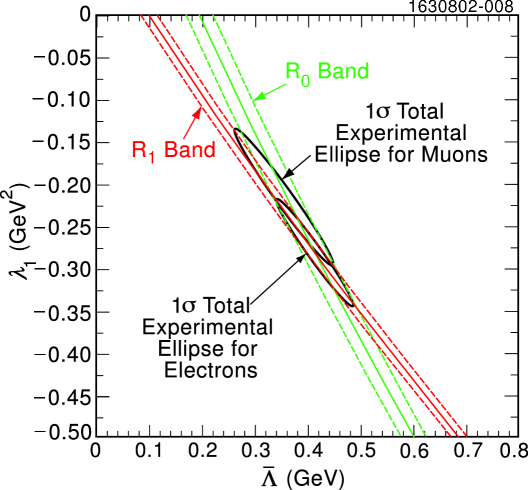
Рис. 10: Constrains on the HQET parameters $\lambda_{1}$ and $\bar{\Lambda}$ from measurements of the moments R₀ and R₁. The contours represent $\Delta\chi^{2}=1$ for the combined statistical and systematic errors on the measured values.

Using the expression of the full semileptonic decay width given in Eq. (95) and the experimental value $\Gamma_{SL}^{exp}=(0.43\pm 0.01){\times}10^{-10}$ MeV [10], one can extract $|{\mbox{V}}_{cb}|$:

$$|{\mbox{V}}_{cb}|=(40.8\pm 0.5|_{\Gamma_{SL}}\pm 0.4|_{\lambda_{1},\bar{\Lambda}}\pm 0.9|_{th})\times 10^{-3},$$ (104)

where the first uncertainty is from the experimental value of the semileptonic width, the second uncertainty is from the HQET parameters (${\lambda}_{1}$ and $\bar{\Lambda}$), and the third uncertainty is the theoretical one. Non-quantified uncertainties are associated with a possible quark-hadron duality violation.

4.4. $|V_{ub}|$

The methods which are currently available for probing $V_{ub}$ are unfortunately plagued by dependence on phenomenological models whose uncertainties are difficult to quantify reliably. As a result, despite many experimental efforts present constraints on this parameter are unacceptably weak. The analyses which have been used fall into two classes, inclusive decays of the form $B\to X_{u}l\nu$, and exclusive transitions such as $B\to(\pi,\rho)l\nu$.

The inclusive decay rate has the advantage that it can be predicted in the form of a systematic expansion in powers of $1/m_{b}$. Experimentally measurements of $b\to u\ell\nu$ which are sensitive to $|V_{ub}|$ are difficult due to the overwhelming background from the Cabibbo favored $b\to c\ell\nu$ decays. At present, this background can be suppressed only by confining oneself to kinematic regions in which only charmless final states can contribute, such as $E>2.2\,$GeV or $M(X)<1.9\,$GeV. Unfortunately, the OPE techniques which allow one to calculate reliably the total inclusive rate breaks down when the phase space is restricted in this way. Phenomenological models must then be used to reconstruct the rate in the unobserved kinematic regions, and the model independence of the analysis is lost.

The inclusive analysis includes a wide kinematic range to avoid losing signal statistics but then pays the price of quark-hadron duality and a fine-tuned modeling of charm backgrounds. Combining the observed yield of lrptons in the end-point momentum interval 2.2-2.6 GeV/c with the recent data on $B\to X_{s}\gamma$ and using HQET CLEO [47] report the value of

$$|V_{ub}|=(4.08\pm 0.34\pm 0.44\pm 0.16\pm 0.24)\times 10^{-3},$$ (105)

where the first two uncertainties are experimental and the last two are from the theory.

Exclusive transitions are easier to study experimentally. On the other hand theoretical predictions of exclusive decay channels are polluted by the ignorance of the physics of quark hadronization. CLEO restricts itself to exclusive final states ($B\to\pi l\nu$, $\rho l\nu$) using $\nu$-reconstruction, in which there is a more favorable signal-to-noise but a considerable uncertainty in the form-factors. The CLEO exclusive result

$$|V_{ub}|=(3.25\pm 0.30\pm 0.55)\times 10^{-3},$$ (106)

in which the first error is experimental and the second is theoretical, is consistent with that obtained from inclusive measurements.

4.5. Conclusions

At present our knowledge of $\lambda_{1}$ and $\bar{\Lambda}$ limits the precision we can achieve on from inclusive semileptonic $B$ decays. The aim of the new inclusive analyses is to determine $\lambda_{1}$ and $\bar{\Lambda}$ from experiment and thereby decrease the theoretical uncertainty which comes when extracting $|V_{cb}|$ from $\Gamma_{SL}$. Each analysis alone provides two constraints, allowing a measurement of $\bar{\Lambda}$ and $\lambda_{1}$. Combining the two analyses over-constrains the theory parameters thus allowing a test of the theoretical framework and experimental understanding of $b$-quark decays.

While experimental errors have reached $1-2\%$ level, the dominant uncertainties remain of theoretical origin. High precision tests of HQET, checks on possible violations of quark-hadron duality in semileptonic decays. Experimental determination of $m_{b}$, $m_{b}-m_{c}$ and $\lambda_{1}$ are needed to complete this challenging experimental program.

5. A bit of phenomenology. Electron spectra in semileptonic $B$ and $B_{c}$ decays.

Electron energy spectrum in inclusive $B\to X_{c}\ell\nu$ decays can be also treated using OPE. The result (away from the endpoint of the spectrum) is that the inclusive differential decay width $d\Gamma/dE$ may be expanded in $\Lambda/m_{b}$. The leading term (zeroth order in $\Lambda/m_{b}$) is the free quark decay spectrum, the subleading term vanishes, and the subsubleading term involves parameters from the heavy quark theory, but should be rather small, as it is of order $(\bar{\Lambda}/m_{b})^{2}$.

However, the calculation of the lepton energy spectrum in OPE shows the appearance of singular distributions $\delta^{(n)}(E-m_{b}/2)$ near the end point where $E=m_{b}/2$. The non adequacy of the approach is also evident from the fact that although $m_{b}/2$ is the largest lepton energy available for a free quark decay, the physical endpoint corresponds to $E=m_{B}/2$. In this windows bound state effects, due to the Fermi motion of the heavy quark, become important and the $1/m_{b}$ expansion has to be replaced by an expansion in twist. To describe this region one has to introduce a so–called ‘‘shape function’’ [51], [52] which in principle introduces a hadronic uncertainty. This is quite analogous to what happens for the structure function in deep–inelastic scattering in the region where the Bjorken variable $x_{B}\to 1$. A model independent determination of the shape function is not available at the present time, therefore a certain model dependence in this region seems to be unavoidable, unless lattice data become reasonably precise.

Two phenomenological approaches had been applied to describe strong interaction effects in the inclusive weak decays: the parton ACM model [53] amended to include the motion of the heavy quark inside the decaying hadron, and the ‘‘exclusive model’’ based on the summation of different channels, one by one [54].

The various light–front (LF) approaches to consideration of the inclusive semileptonic transitions were suggested in Refs. [55]–[58]. In Refs. [55], [56] the Infinite Momentum Frame prescription $p_{b}=xp_{B}$, and, correspondingly, the floating $b$ quark mass $m_{b}^{2}(\xi)=x^{2}m_{B}^{2}$ have been used. The transverse $b$ quark momenta were consequently neglected. In Ref. [58] the $b$–quark was considered as an on–mass–shell particle with the definite mass $m_{b}$ and the effects arising from the $b$–quark transverse motion in the $\bar{B}$–meson were included. The corresponding ansätz of Ref. [58] reduces to a specific choice of the primordial LF distribution function $|\psi(\xi,p^{2}_{\bot})|^{2}$, which represents the probability to find the $b$ quark carrying a LF fraction $\xi$ and a transverse momentum squared $p^{2}_{\bot}=|{\bf p}_{\bot}|^{2}$. As a result, a new parton–like formula for the inclusive semileptonic $b\to c,u$ width has been derived [58], which is similar to the one obtained by Bjorken et al. [59] but in case of infinitely heavy $b$ and $c$ quarks.

5.1. ACM model

The ACM model was originally developed to consider in detail the endpoint of the lepton spectrum in order to estimate a systematic error in modeling the full spectrum. It incorporates some of the corrections related to the fact that the decaying $b$ quark is not free, but in a bound state. It was explicitly constructed to avoid mention of a $b$ quark mass. The model is extensively used in the analysis of the lepton energy spectrum in semi-leptonic decays. It reproduces very well numerically the shape of the semi-leptonic spectra at least in its regular part.

The model treats the $B$ meson with the mass $m_{B}$ as consisting of the heavy $b$ quark plus a spectator with fixed mass $m_{sp}$; the latter usually represents a fit parameter. The spectator quark has a momentum distribution $\Phi({\bf p}^{2})$ (${\bf p}$ is its three-dimensional momentum). The momentum distribution is usually taken to be Gaussian: normalized so that

$$\int\Phi({\bf p}^{2})p^{2}dp=1.$$ (107)

The decay spectrum is determined by the kinematics constrains on the $b$ quark. The energy-momentum conservation in the $B$ meson vertex implies that the $b$ quark energy is

$$E_{b}=m_{B}-\sqrt{{\bf p}^{2}+m_{sp}^{2}},$$ (108)

thus the $b$ quark cannot possess a definite mass. Instead, one obtains a ‘‘floating’’ $b$ quark mass

$$(m_{b}^{f})^{2}=m_{B}^{2}+m_{sp}^{2}-2m_{B}\sqrt{{\bf p}^{2}+m_{sp}^{2}},$$ (109)

which depends on $|{\bf p}|^{2}$. The lepton spectrum is first obtained from the spectrum $d\Gamma_{b}^{(0)}(m_{f},E)/dE$ of the $b$ quark of invariant mass $m_{b}^{f}$ (in the $b$ quark rest frame)

$${d\Gamma_{b}^{(0)}(m_{b},E)\over dE}={G_{F}^{2}m_{b}^{4}\over 48\pi^{3}}{x^{2}(x_{max}-x)^{2}\over(1-x)^{3}}\left[(1-x)(3-2x)+(1-x_{max})(3-x)\right]$$ (110)

with $x={2E_{e}/m_{b}}$, $x_{max}=1-\rho$, and $\rho={m_{c}^{2}/m_{b}^{2}}$, then boosting back to the rest frame of the $B$ meson and averaging over the weight function $\Phi({\bf p}^{2})$ .

$${d\Gamma_{B}\over dE}=\int\limits_{0}^{p_{max}}dpp^{2}\Phi({\bf p}^{2}){(m_{b}^{f})^{2}\over 2pE_{b}}\int_{E_{-}}^{E_{+}}{dE^{\prime}\over E^{\prime}}{d\Gamma^{(0)}_{b}(m_{f},E^{\prime})\over dE^{\prime}}\leavevmode\nobreak\ .$$ (111)

The perturbative corrections are neglected for the moment. In Eq. (111)

$$p_{max}=\frac{m_{B}}{2}-\frac{m_{c}^{2}}{2m_{B}-4E}\leavevmode\nobreak\ ,\leavevmode\nobreak\ \leavevmode\nobreak\ \leavevmode\nobreak\ E_{\pm}=\frac{Em_{b}^{f}}{E_{b}\mp|{\bf p}|}\leavevmode\nobreak\ .$$ (112)

In fact the upper limit of integration in (111) is not $E^{+}$ but ${\it min}(E_{+},E_{max})$, where

$$E_{max}=\frac{m_{B}-m_{sp}}{2}\left(1-\frac{m_{c}^{2}}{(m_{B}-m_{sp})^{2}}\right).$$ (113)

These expressions conclude the kinematical analysis in the ACM model.

5.2. B-meson on the Light-Front

The elegance and simplicity of the Light-Front (LF) approach results from the analogy uf relativistic field theories quantized in the LF to non-relativistic quantum mechanics. In fact this correspondence runs deep and there is exact isomorphism between the Galilean subgroup of the Poincaré group and the symmetry group of two dimensional quantum mechanics. LF theory also provides a support for the intuitive quark-parton picture of bound states in QCD. The purpose of this subsection is to illustrate the attractive feature of the Lf approach in the simplest fashion by working out a concrete example of inclusive semileptonic $B$ decays [58]. Other applications can be found in [34],[60].

Similar to the ACM model the LF quark model treats the beauty meson as consisting of the heavy $b$ quark plus a spectator quark. Both quarks have fixed masses, $m_{b}$ and $m_{sp}$, though. This is at variance with the ACM model, that has been introduced in order to avoid the notion of the heavy quark mass at all. The calculation of the distribution over lepton energy in the LF approach does not requires any boosting procedure but is based on the standard Lorentz–invariant kinematical analysis.

There are three independent kinematical variables in the inclusive phenomenology: the lepton energy $E_{\ell},q^{2}$, where $q=p_{\ell}+p_{\nu_{\ell}}$, and the invariant mass $M^{2}_{X}=(p_{B}-q)^{2}$ of a hadronic state. Introducing the dimensionless variables $y=2E_{\ell}/m_{B}$, $t=q^{2}/m^{2}_{B}$, and $s=M^{2}_{X}/m^{2}_{B}$, the differential decay rate for semileptonic $B$ decay can be written as

$$\frac{d\Gamma_{SL}}{dy} = \frac{G_{F}^{2}m_{B}^{5}}{64\pi^{3}}|V_{cb}|^{2}\int\limits^{t_{max}}_{0}dt\int\limits^{s_{max}}_{s_{0}}ds$$

$$\times\left\{tW_{1}+\frac{1}{2}[y(1+t-s)-y^{2}-t]W_{2}+t[\frac{1+t-s}{2}-y]W_{3}+\ldots\right\},$$

where the structure functions $W_{i}=W_{i}(s,t)$ appear in the decomposition of the hadronic tensor $W_{\alpha\beta}$ in Lorentz covariants. The ellipsis in (5.2.) denote the terms proportional to the lepton mass squared. The kinematical limits of integration can be found from equation

$$\frac{s}{1-y}+\frac{t}{y}\leq 1$$ (115)

They are given by $0\leq y\leq(1-\rho)$, where $\rho=m_{c}^{2}/m_{b}^{2}$, $s_{max}=1+t-(y+t/y)$, and $t_{max}=y[1-\rho/(1-y)]$.

In a parton model LF inclusive semileptonic $B_{c}\to X_{Q^{\prime}}\ell\nu_{\ell}$ decay is treated in a direct analogy to deep-inelastic scattering. An approach is based on the hypothesis of quark–hadron duality. This hypothesis assumes that the inclusive decay probability for which no reference to a particular hadronic state is needed equals to one into the free quarks. The basic ingredient is the expression for the hadronic tensor $W_{\alpha\beta}$ which is given through the optical theorem by the imaginary part of the quark box diagram describing the forward scattering amplitude:

$$W_{\alpha\beta}=\int L^{(cb)}_{\alpha\beta}(p_{c},p_{b})\delta[(p_{b}-q)^{2}-m_{c}^{2}]\frac{|\psi(\xi,p^{2}_{\bot})|^{2}}{\xi}\theta(\varepsilon_{c})d\xi d^{2}p_{\bot},$$ (116)

where a quark tensor $L^{(cb)}_{\alpha\beta}(p_{c},p_{b})$ is defined as

$$L^{cb}_{\alpha\beta}(p_{c},p_{b})=\frac{1}{4}\sum_{spins}\bar{u}_{c}O_{\alpha}u_{b}\cdot\bar{u}_{b}O^{+}_{\beta}u_{c}=2(p_{c\alpha}p_{b\beta}+p_{c\beta}p_{b\alpha}-g_{\alpha\beta}(p_{c}p_{b})+i\epsilon_{\alpha\beta\gamma\delta}p^{c\gamma}p^{b\delta})$$ (117)

and the factor $1/\xi$ in Eq. (116) comes from the normalization of the $B$ meson vertex [60].

Eq. (116) amounts to averaging the perturbative decay distribution over motion of heavy quark governed by the distribution function $|\psi(\xi,p^{2}_{\bot})|^{2}$. In this respect the approach is similar to the parton model in deep inelastic scattering, although it is not really a parton model in its standard definition. The normalization condition reads

$$\pi\int\limits_{0}^{1}d\xi\int dp^{2}_{\bot}|\psi(\xi,p^{2}_{\bot})|^{2}=1.$$ (118)

The function $\theta(\varepsilon_{c})$ where $\varepsilon_{c}$ is the $c$–quark energy is inserted in Eq. (116) for consistency with the use of valence LF wave function to calculate the $b$–quark distribution in the $B$–meson.

Recall that the endpoint for the quark decay spectrum is

$$y_{max}^{b}=(m_{b}/m_{B})(1-m_{c}^{2}/m_{b}^{2}),$$ (119)

whereas the physical endpoint is

$$y_{max}=1-m^{2}_{D}/m_{B}^{2}.$$ (120)

where $m_{D}$ is the $D$ meson mass. The endpoint for the LF electron spectrum is in fact not $y_{max}$ but

$$y_{max}^{LF}=1-m^{2}_{c}/m_{B}^{2}.$$ (121)

This is the direct consequence of the $p^{2}_{\bot}$ integration in Eq. (129) [58]. Note that $y_{max}^{LF}$ coincides with $y_{max}^{ACM}$ with accuracy $\sim m_{sp}/m_{B}$. For $m_{c}\sim 1.5$ GeV the difference between $y_{max}^{LF}$ and $y_{max}$ is of the order $10^{-2}$.

5.3. The distribution function of the $b$ quark

An explicit representation for the $B$-meson Fock expansion in QCD is not known. A priory, there is no connection between equal–time (ET) wave function $w({\bf k}^{2})$ of a constituent quark model and LF wave function $\psi(x,p^{2}_{\bot})$. The former depends on the center–of–mass momentum squared $k^{2}=|{\bf k}|^{2}$, while the latter depends on the LF variables $\xi$ and $p_{\bot}^{2}$. However, there is a simple operational connection between ET and LF wave functions [61]. This is model dependent enterprise but has its close equivalent in studies of electron spectra using the ACM model. The idea is to find a mapping between the variables of the wave functions that will turn a normalized solution $w({\bf k}^{2})$ of the ET equation of motion into a normalized solution $\psi(\xi,p^{2}_{\bot})$ of the different looking LF equation of motion. That will allows us to convert the ET wave function, and all the labor behind it, into a usable LF wave function. This procedure amounts to a series of reasonable (but naive) guesses about what the solution of a relativistic theory involving confining interactions might look like.

Specifically, one converts from ET to LF momenta by leaving the transverse momenta unchanged, ${\bf k}_{\bot}={\bf p}_{\bot}$ and letting

$$p_{iz}=\frac{1}{2}(p_{i}^{+}-p_{i}^{-})=\frac{1}{2}(p_{i}^{+}-\frac{p^{2}_{i{\bot}}+m^{2}_{i}}{p_{i}^{+}})$$ (122)

for both the $b$–quark $(i=b)$ and the quark–spectator $(i=sp)$. Here $p_{i}^{\pm}=p_{i0}\pm p_{iz}$ with $\sum p_{i}^{+}=p_{B}^{+}=m_{B}$ (in the B meson rest frame).

In what follows we identify $\Phi({\bf k}^{2})=|w({\bf k}^{2})|^{2}$ with the Gaussian distribution

$$\Phi({\bf k}^{2})={4\over\sqrt{\pi}p_{F}^{3}}\exp\left(-\frac{{\bf k}^{2}}{p_{F}^{2}}\right).$$ (123)

The simple calculation yields

$$|\psi(\xi,p^{2}_{\bot})|^{2}=\frac{4}{\sqrt{\pi}p^{3}_{f}}\exp\left(-\frac{p^{2}_{\bot}+p^{2}_{z}}{p^{2}_{f}}\right)\left|\frac{\partial p_{z}}{\partial\xi}\right|,$$ (124)

where

$$p^{2}_{z}(\xi,p^{2}_{\bot})=\frac{1}{2}\left((1-\xi)m_{B}-\frac{p^{2}_{\bot}+m^{2}_{{\rm sp}}}{(1-\xi)m_{B}}\right),\leavevmode\nobreak\ \leavevmode\nobreak\ \leavevmode\nobreak\ \xi=\xi_{{\rm sp}},$$ (125)

and

$$\left|\frac{\partial p_{z}}{\partial\xi}\right|=\frac{1}{2}\left(m_{B}+\frac{p^{2}_{\bot}+m^{2}_{{\rm sp}}}{(1-\xi)^{2}m_{B}}\right).$$ (126)

The calculation of the structure functions $W_{i}(t,s)$ in the LF parton approximation (116) is straightforward. The result is

$$W_{i}(t,s)=\int w_{i}(s,t,\xi)\delta[(p_{b}-q)^{2}-m_{c}^{2}]\frac{|\psi(\xi,p^{2}_{\bot})|^{2}}{\xi}\theta(\varepsilon_{c})d\xi d^{2}p_{\bot},$$ (127)

where the structure functions $w_{i}(s,t,\xi)$ are defined in the same way as $W_{i}(s,t)$ in (5.2.) but for the free quark decay. Explicit expressions for $W_{i}(s,t)$ can be obtained using Eq. (117), they are given in Ref. [58]. Eq. (127) differs from the corresponding expressions of Refs. [55] and [56] by the non–trivial dependence on $p^{2}_{\bot}$ which enters both $|\psi(\xi,p^{2}_{\bot})|^{2}$ and argument of the $\delta$–function. For further details see [58].

5.4. The choice of $m_{b}$

An important technical issue that appear in the problem is the definition of the quark mass $m_{b}$. The semileptonic decay rate is proportional to $m_{b}^{5}$, thus any uncertainty in the definition of heavy quark mass transfers into a huge uncertainty in the predicted rate. The problem is to find a definition consistent with that of HQET.

In the ACM model, it is known [62], [63] that once the semileptonic width $\Gamma_{{\rm ACM}}$ is expressed in terms $m_{b}^{ACM}\leavevmode\nobreak\ =\leavevmode\nobreak\ <m_{b}^{f}>$ (that is nothing but the floating mass $m_{b}^{f}({\bf p}^{2})$ of Eq. (109) averaged over the distribution $\Phi({\bf p}^{2}$) ), the correction to first order in $1/m_{b}$ both to the inclusive semileptonic width and to the regular part of the lepton spectrum can be absorbed into the definition of the quark mass, in full agreement with the general HQET statement of the absence of the $1/m_{b}$ correction in total width.

The choice of $m_{b}$ in the LF approach was first addressed in the context of the LF model for $b\to s\gamma$ transitions [64]. It was shown that the LF model can be made agree with HQET provided $m_{b}^{LF}$ is defined from the requirement of the vanishing of the first moment of the distribution function. This condition coincides with that used in HQET to define the pole mass of the $b$–quark. In this way one avoids an otherwise large (and model dependent) correction of order $1/m_{b}$ but at expense of introducing the shift in the constituent quark mass which largely compensates the bound state effects. It has been also demonstrated that the values of $m_{b}^{LF}$ found by this procedure agree well with the average values $<m_{b}^{f}>$ in the ACM model. Accepting the identification $m_{b}^{LF}=m_{b}^{ACM}$, the similar agreement but for the semileptonic $b\to c$ decays has been found in Ref. [65].

5.5. Electron energy spectra. LF model vs ACM model

In Table 4 for various values of $p_{F}$, the values of the total semileptonic width for the free quark with the mass $m_{b}=<m_{b}^{f}>$ and the $B$ meson semileptonic widths, calculated using the LF and ACM approaches, respectively, are given. In the last two columns, shown are the fractional deviation $\delta=\Delta\Gamma_{SL}/\Gamma_{SL}^{b}$ (in per cent) between the semileptonic widths determined in the LF and ACM models and that of the free quark. The agreement between the LF and ACM approaches for integrated rates is excellent for small $p_{F}$. This agreement is seen to be breaking down at $p_{F}\geq 0.4$ GeV, but even for $p_{F}\sim 0.5$ GeV the difference between the ACM and LF inclusive widths is still small and is of the order of a per cent level.

$p_{F}$	$<m_{b}^{f}>$	$\Gamma_{SL}^{b}$	$\Gamma_{SL}^{ACM}$	$\Gamma_{SL}^{LF}$	$\delta^{ACM}$	$\delta^{LF}$
0.1	5.089	0.1007	0.1005	0.1005	0.2	0.2
0.2	5.004	0.0906	0.0902	0.0901	0.4	0.5
0.3	4.905	0.0799	0.0792	0.0789	0.9	1.2
0.4	4.800	0.0696	0.0688	0.0682	1.1	2.0
0.5	4.692	0.0602	0.0592	0.0584	1.7	3.0

Таблица 4: Comparison of the LF and ACM results for the semileptonic integrated rates. In all cases $m_{sp}=0.15$ GeV and $m_{c}=1.5$ GeV and the radiative corrections are neglected. A momentum distribution of the b-quark is taken in the standard Gaussian form (123) with the Fermi momentum $p_{F}$. $|V_{cb}|=0.04$.

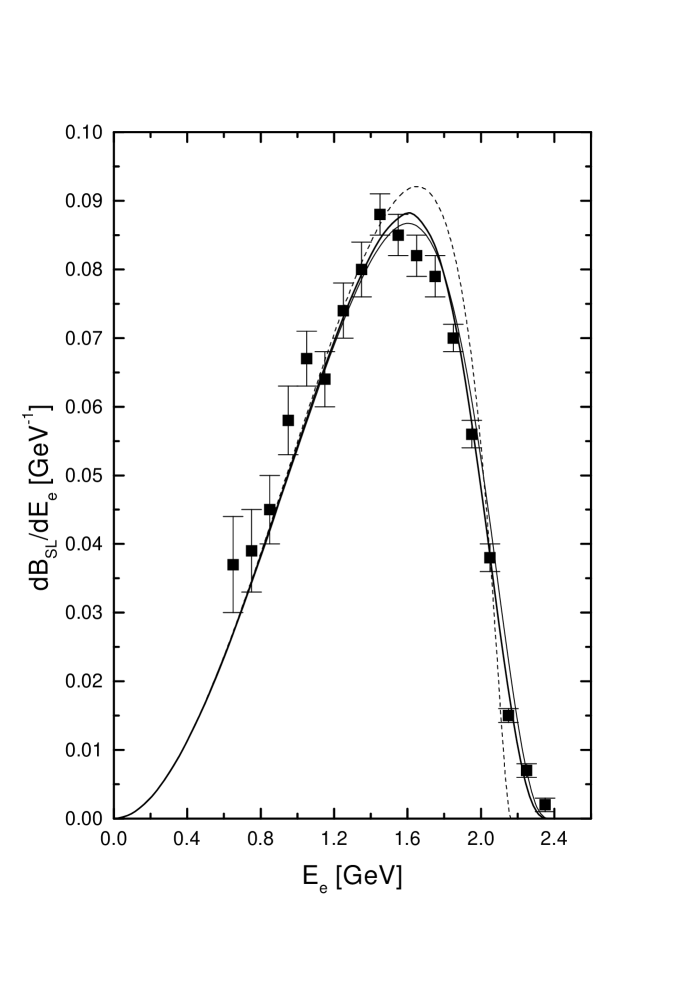
Рис. 11: The predicted electron energy spectrum compared with the CLEO data [43]. The calculation uses $p_{f}=0.4$ GeV, $m_{b}=4.8$ GeV, $m_{c}=1.5$ GeV, and $\alpha_{s}=0.25$ for the perturbative corrections. Thick solid line is the LF result, thin solid line is the ACM result, dashed line refers to the free quark decay. The spectra normalized to $10.16\%$, $10.23\%$, and $10.36\%$, respectively. $|V_{cb}|=0.042$.

Fig. 11 shows the three theoretical curves for electron spectrum in inclusive $B\to X_{c}\ell\nu_{\ell}$ decays are presented for the LF, ACM and free quark models. This is a direct calculation of the spectrum and not a $\chi^{2}$ fit. A more detailed fit can impose constrains on the distribution function and the mass of the charm quark. Such the fit should also account for detector resolution. The overall normalization of the electron energy spectra is

$$BR_{LF}=10.16\%,\leavevmode\nobreak\ \leavevmode\nobreak\ \leavevmode\nobreak\ BR_{ACM}=10.23\%\leavevmode\nobreak\ \leavevmode\nobreak\ \leavevmode\nobreak\ BR_{free}=10.37\%,$$ (128)

in agreement with the experimental finding [43] $BR_{SL}=(10.49\pm 0.17\pm 0.43)\%$.

The calculations implicitly include the ${\it O}(\alpha_{s})$ perturbative corrections arising from gluon Bremsstrahllung and one–loop effects which modify an electron energy spectra at the partonic level (see e.g. [66] and references therein). It is customary to define a correction function $G(x)$ to the electron spectrum $d\Gamma_{b}^{(0)}$ calculated in the tree approximation for the free quark decay through

$$\frac{d\Gamma_{b}}{dx}=\frac{d\Gamma^{(0)}_{b}}{dx}\left(1-\frac{2\alpha_{s}}{3\pi}G(x)\right),$$ (129)

where $x=2E/m_{b}$. The function $G(x)$ contains the logarithmic singularities $\sim\ln^{2}(1-x)$ which for $m_{c}=0$ appear at the quark-level endpoints $x_{max}=1$. This singular behaviour at the end point is clearly a signal of the inadequacy of the perturbative expansion in this region. The problem is solved by taking into account the bound state effects [55]. Since the radiative corrections must be convoluted with the distribution function the endpoints of the perturbative spectra are extended from the quark level to the hadron level and the logarithmic singularities are eliminated.

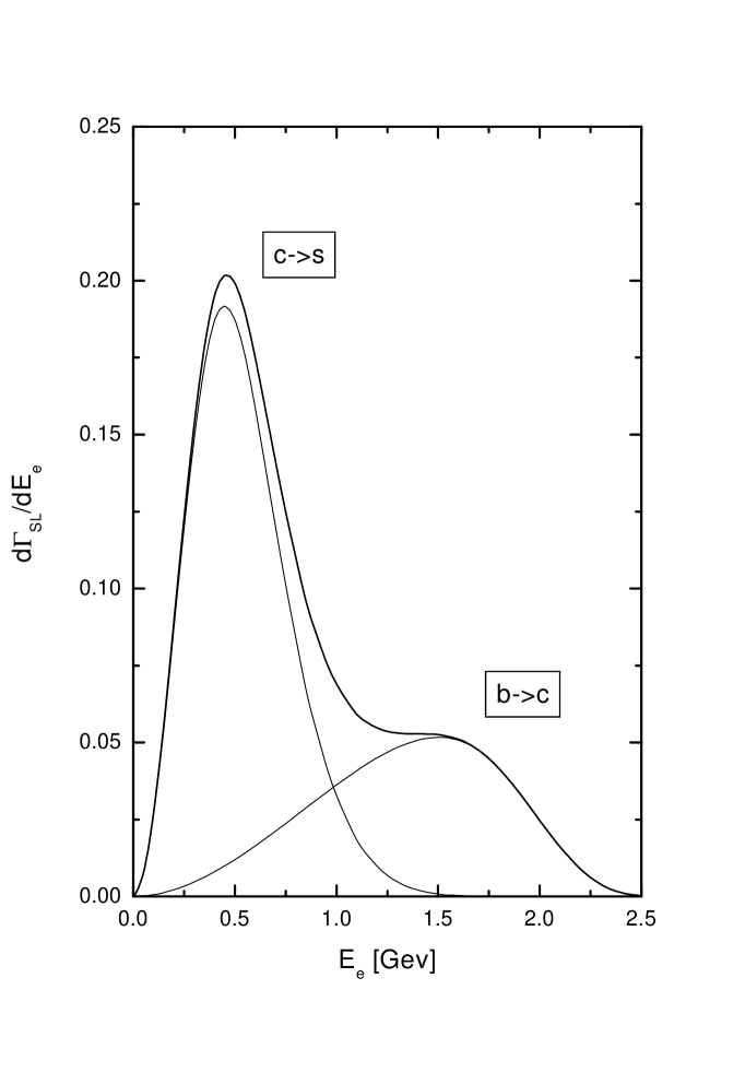
Рис. 12: The predicted electron energy spectrum in semileptonic $B_{c}$ decays. The calculation uses $p_{F}=0.92$ GeV, $m_{b}=5.0$ GeV, $m_{c}=1.5$ GeV, and $\alpha_{s}=0.25$ for the perturbative corrections.

5.6. $B_{c}$ decays

The semileptonic decay of $B_{c}$ consists of two contributions, $\Gamma_{SL}=\Gamma_{SL}^{b}+\Gamma_{SL}^{c}$. which are, respectively. $b\to\bar{c}W^{+}$ with $c$-quark as spectator and $\bar{c}\to\bar{s}W^{-}$ with $b$ quark as spectator. Since these processes lead to different the final states, their amplitudes do not interfere. In the simplest view, $b$ and $\bar{c}$ are free, and the total semileptonic width is just the sum of the $b$ and $\bar{c}$ semileptonic widths, with $c$-decay dominating. Approximating this by $\Gamma_{SL}(B_{c})=\Gamma_{SL}(B)+\Gamma_{SL}(D)$ yields $\Gamma_{SL}(B_{c})\sim 0.22$ ps^-1. This estimate is modified by strong interaction effects.

Fig. 12 shows the lepton energy spectrum in the decay $B_{c}\to Xe\nu_{e}$. This calculation refers to the case $m_{b}=5$ GeV, $m_{c}=1.5$ GeV as chosen in Ref. [68]. The free quark semileptonic widts are $\Gamma_{SL}^{c,free}=0.218$ ps^-1, and $\Gamma_{SL}^{b,free}=0.090$, ps^-1. The Fermi momentum $p_{F}$ is chosen as $p_{F}=0.92$ GeV corresponding to the Isgur-Scora Model. Like the OPE formalism the LF approach leads to a reduction of the free quark decay rates caused by binding, $\Gamma_{SL}^{b,bound}=0.090$, ps^-1 $\Gamma_{SL}(B_{c})=0.18$ ps^-1, but the bound state corrections for $c\to s$ semileptonic rate are substantially larger than those reported in [68]. The result of Ref. [68] would correspond to a very soft $B_{c}$ wave function with $p_{F}\sim 0.5$ GeV, which is seemed to be excluded by existing constituent quark models.

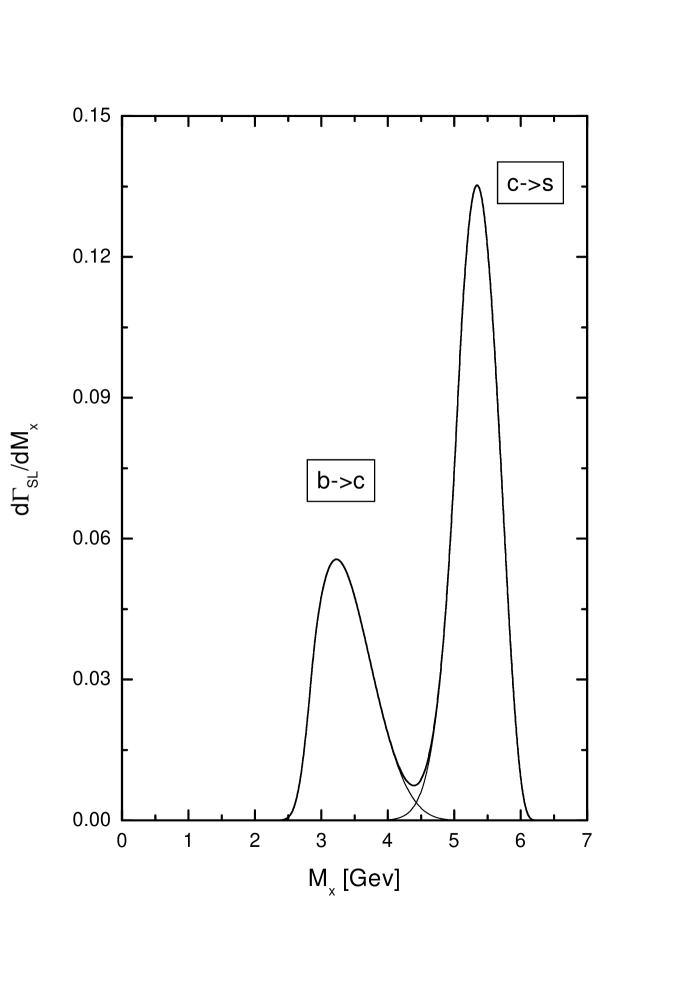
Рис. 13: The predicted hadronic mass distribution spectrum in semileptonic $B_{c}$ decays. The calculation uses $p_{F}=0.92$ GeV, $m_{b}=5.0$ GeV, $m_{c}=1.5$ GeV

Finally, we note that the theoretical results for the electron spectrum can be translated into predictions for the hadronic mass spectrum. In Fig. 13 we show the invariant mass distribution of the hadrons recoiling against $\ell\nu$. The LF predictions for hadronic mass spectra must be understood in the cense of quark–hadron duality. The true hadronic mass spectrum may have resonance structure that looks rather different from inclusive predictions. Inclusive calculations predict a continuum which is given by the inclusive spectrum and is dual to a large number of overlapping resonances.

References

- [1] Cabibbo N, Phys. Rev. Lett. 10, 531 (1963); Kobayashi M. and Maskawa T., Prog. Theo. Phys. 49, 652 (1973)
- [2] Buras A., CP violation in B and K decays, Lectures given at the 41 Schladming School in Theoretical Physics, Schladming, February 22-28, 2003, arXiv: hep-ph/0307293
- [3] Glashow S,, Iliopoulos J., Maiani L., Phys. Rev. D2, 1285 (1970)
- [4] Albrecht, H,. et al., Argus collaboration, Phys. Lett., B192, 245 (1997)
- [5] Aubert B. et al. [BaBar Collaboration], Improved measurement of the CP-violating asymmetry amplitude sin2beta, arXiv: hep-ex/0203007
- [6] Abe K. et al. [Belle Colaboration], Phys. Rev. D66 032007 (2002)
- [7] Quinn E., B physics and CP violation, Lectures given at Particle Physics School, ICTP, Trieste, July 2001, arXiv: hep-ph/0111177
- [8] Nir Y., CP violation: A New Era, Lectures given at the 55th Scottish University Summer School in Physics, St.Andrews, Scottland, August 7-20, 2001, arXiv: hep-ph/0109090
- [9] Neubert M., arXiv: hep-ph/0110304; Nir Y., arXiv: hep-ph/0208080
- [10] Artuso M. and Barberio E., ref. [12] [arXiv: hep-ph/0205163]
- [11] Altarelli G., Feruglio F., to be published in Proceedings of the X International Workshop on Neutrino Telescopes, March 11-14 2003, Venezia, Italy, arXiv: hep-ph/0306265
- [12] Hagiwara K. et al., (Particle Data Group), Phys. Rev. D 66, 010001 (2002)
- [13] Jarlskog C., Phys. Rev. Lett. 55, 1039 (1985)
- [14] Ahmed S. et al. [CLEO Collaboration], arXiv: hep-ex/9908022.
- [15] Barate R. et al. [ALEPH Collaboration], Phys. Lett. B429, 169 (1998).
- [16] Greub C. and Hurth T., Nucl. Phys. (Proc. Suppl.) B74, 247 (1999) [arXiv: hep-ph/9809468].
- [17] Wolfenstein L., Phys. Rev. Lett. 51, 1945 (1983).
- [18] Buras A.J., Lautenbacher M.E. and Ostermaier G., Phys. Rev. D50, 3433 (1994) [arXiv: hep-ph/9403384]
- [19] Buras A.J. and Fleishner R, in ‘‘Heavy Flavors II,’’ eds. Buras A.J. and Linder M., World Scientific, Singapore 1998
- [20] Höcker A., Lacker H., Laplace S., and Le Diberder F., ‘‘A new approach to a global fit of the CKM matrix,’’ Eur. Phys. J. C 21, 225 (2001)
- [21] Vysotsky M., arXiv: hep-ph/0307218
- [22] Schneider O., ref. [12] [arXiv :hep-ph/0206171]
- [23] Gronau M and Rosner J.L., Phys. Rev. D53, 2516 (1996); Phys. Rev. Lett., 76 1200 (1996).
- [24] Luo Z.and Rosner J.L., Phys. Rev. D65 054027 (2002).
- [25] Charles J., Phys. Rev, D59, 054007 (1999).
- [26] Rosner J.L., arXiv: hep-ph/0305315
- [27] BaBar collaboration, Aubert. B. et al., Phys. Rev. Lett. 89, 281802(2002).
- [28] Belle collaboration, Abe, K. et al, Phys. Rev., D68, 012001 (2003).
- [29] Briere R.A. et al., CLEO Collaboration, Phys.Rev.Lett. 89 081803 (2002), arXiv: hep-ex/0203032.
- [30] Abe K. et al. (Belle collaboration), Phys. Lett, B526, 247 (2002) [arXiv: hep-ex/0111060].
- [31] Buskulic D.et al. (ALEPH collaboration), Phys. Lett. B335, 373 (1997)
- [32] Abreu P. et al. (DELPHI collaboration), Phys. Lett. B 510, 55 (2001).
- [33] Abbiendi G. et al. (OPAL collaboration), Phys. Lett. B 482, 15 (2000)
- [34] Demchuk N.B., Kulikov P.Yu, Narodetskii I.M., O’Donnell P.J., Phys. Atom. Nucl. 60 1292 (1997); Yad. Fiz. 60, 1429 (1997)
- [35] Isgur N. and Wise M.B., Phys. Lett. B232, 113 (1989); Phys. Lett. B237, 527 (1990).
- [36] Neubert M. and Wise M.B., Heavy-Quark Physics, Cambridge University Press, Cambridge 2000
- [37] Luke M., Phys. Lett. B 252, 447 (1990)
- [38] Scora D. and Isgur N., Phys. Rev. D52, 2783 (1995).
- [39] Ligeti Z., Nir Y. and Neubert M., Phys. Rev. D49, 1302 (1994).
- [40] Hashimoto S. et al., Phys. Rev. D61, 014502 (1999)
- [41] Aubert B. et al. CLEO collaboration, Phys.Rev. D67, 031101 (2002) [arXiv: hep-ex/0208018]
- [42] Albrecht H. et al. ARGUS collaboration, Phys. Lett. B318, 377 (1993)
- [43] Barish B. et al., CLEO collaboration, Phys. Rev. Lett. 76, 1570 (1995)
- [44] Bigi I., Shifman M., and Uraltsev N.G., Annu. Rev. Nuc. Part. Sci., 47, 591 (1997).
- [45] Bigi I. and Uraltsev N.G., Int.J.Mod.Phys. A16, 5201 (2001)
- [46] Isgur N., Phys. Lett. B448, 111 (1999)
- [47] Bomheim A.et al.) (CLEO collaboration), Phys. Rev. Lett. 88, 231803-1 (2002)
- [48] Chen S. et al., CLEO collaboration, Phys.Rev.Lett. 87 251807 (2001) [arXiv: hep-ex/0108032]
- [49] Gremm M. and Kapustin A., Phys. Rev. D55, 6924 (1997) [arXiv: hep-ph/9603448].
- [50] Briere R.A. et al., CLEO collaboration, arXiv: hep-ex/0209024
- [51] Bigi I. et al., Int. J. Mod. Phys. A9, 2467 (1994)
- [52] Neubert M., Phys. Rev. D49, 3392, 4623 (1994)
- [53] Altarelli G., Cabibbo N., Corbo G., Maiani L., and Martinelli G., Nucl. Phys. B202, 512 (1982)
- [54] Isgur N. et al., Phys. Rev. D39, 799 (1989).
- [55] Jin C.H., Palmer M.F., and Paschos E.A., Phys. Lett. B329, 364 (1994)
- [56] Morgunov V.L., Ter-Martirosyan K.A., Phys. Atom. Nucl. 59, 1221 (1996)
- [57] Grach I.L., Narodetskii I.M., Simula S., and Ter-Martirosyan K.A., Nucl. Phys. B592, 227 (1997)
- [58] Kotkovsky S., Narodetskii I.M., Simula S., and Ter-Martirosyan K.A., Phys. Rev. D60, 114024 (1999)
- [59] Bjorken J., Dunietz I., and Taron M., Nucl. Phys. A371, 111 (1992)
- [60] Demchuck N.B., Grach I.L., Narodetskii I.M., and Simula S., Phys. At. Nucl. 59, 2152 (1996)
- [61] Coester F., Prog. Part. Nucl. Phys. 29, 1 (1992)
- [62] Randall L. and Sundrum R., Phys. Lett. B312, 148 (1993)
- [63] Bigi I., Shifman M., Uraltsev N.G., Vainstein A., Phys. Lett. B328, 431 (1994)
- [64] Keum Y.-Y., Kulikov P.Yu, Narodetskii I.M., Song H.S., Phys. Lett. B471, 72 (1999)
- [65] Grach I.L., Kulikov P.Yu, Narodetskii I.M., JETP Letters, 73, 317 (2001)
- [66] Jezabek M. and Kühn J.H., Nucl. Phys. B320, 20 (1989)
- [67] Datta A., Kulikov P.Yu., Narodetskii I.M. and O’Donnell P.J., in preparation
- [68] Beneke M, Buchalla G., Phys. Rev. D53, 4991 (1996)