The R-Parity Violating Minimal Supergravity Model111Preprint number : TUM-522/03, LAPTH-997/TH, BONN-TH-2003-04
Abstract
We present the minimal supersymmetric standard model with general broken R-parity, focusing on minimal supergravity (mSUGRA). We discuss the origins of lepton number violation in supersymmetry. We have computed the full set of coupled one-loop renormalization group equations for the gauge couplings, the superpotential parameters and for all the soft supersymmetry breaking parameters. We provide analytic formulæ for the scalar potential minimization conditions which may be iterated to arbitrary precision. We compute the low-energy spectrum of the superparticles and the neutrinos as a function of the small set of parameters at the unification scale in the general basis. Specializing to mSUGRA, we use the neutrino masses to set new bounds on the R-parity violating couplings. These bounds are up-to five orders of magnitude stricter than the previously existing ones. In addition, new bounds on the R-parity violating couplings are also derived demanding a non-tachyonic sneutrino spectrum. We investigate the nature of the lightest supersymmetric particle and find extensive regions in parameter space, where it is not the neutralino. This leads to a novel set of supersymmetric signatures, which we classify.
I Introduction
The most widely studied supersymmetric scenario is the minimal supersymmetric standard model (MSSM) with conserved R-parity Nilles:1983ge ; Kane ; Martin:1997ns . The unification of the three Standard Model gauge couplings, , at the scale Amaldi:1991cn , is a strong indication that supersymmetry (SUSY) is embedded in a unified model. In the simplest such model Nilles:1983ge , SUSY breaking occurs in a hidden sector (decoupled from the Standard Model gauge interactions), and is communicated to our visible sector via gravity foot1 . The scale of SUSY breaking in the visible sector is thus the Planck scale, .
The large number of parameters in the MSSM is restricted by making well-motivated simplifying assumptions at the unification scale. In the special case of the minimal supergravity model (mSUGRA), there are five parameters beyond those of the Standard Model:
| (1) |
These are the universal scalar mass, , gaugino mass, , and trilinear scalar coupling, , respectively, as well as the ratio of the Higgs vacuum expectation values (vev’s), , and the sign of the bi-linear Higgs mixing parameter, . Given these 5 parameters at the unification scale, we can predict the full mass spectrum as well as the couplings of the particles at the weak scale via the supersymmetric renormalization group equations (RGEs). This is the most widely used model for extensive phenomenological and experimental tests of supersymmetry. It is the purpose of this paper to create an analogous model in the case of supersymmetry with broken R-parity (): the R-parity violating minimal supergravity model (-mSUGRA).
The mSUGRA model with universal boundary conditions was first extended to include bi-linear by Hempfling Hempfling:1995wj , focusing on the neutrino sector. A further detailed analysis in this framework was performed by Hirsch et al. Hirsch:2000ef . de Carlos and White were the first to go beyond bi-linear and consider the full set of -couplings deCarlos:1996du ; CW . However, they restricted themselves to the third generation Higgs-Yukawa couplings and used an approximate method to minimize the scalar potential. We detail below how we go beyond this work.
We shall consider the chiral superfield particle content
| (2) |
Here is a generation index, and are and gauge indices, respectively. In supersymmetry, the lepton doublet superfields and the Higgs doublet superfield coupling to the down-like quarks, , have the same gauge and Lorentz quantum numbers (This is an essential feature in our discussion below.). When appropriate we shall combine them into the chiral superfields . The gauge quantum numbers of the chiral superfields and the vector superfields are given in Table 1.
| Chiral Superfields | Components | |||||||||||||
|
|
||||||||||||||
|
|
||||||||||||||
|
|
||||||||||||||
| Vector Superfields | Components | |||||||||||||
I.1 R-Parity Violation
R-parity is defined as the discrete multiplicative symmetry Fayet
| (3) |
where is the spin, the baryon number and the lepton number of the particle. All Standard Model particles including the two scalar Higgs doublets have , their superpartners have . When allowing for R-parity violation, the full renormalizable superpotential is given by Weinberg81
| (4) | |||||
Here YE,D,U are matrices of Yukawa couplings; are Yukawa couplings and are mass-dimension one parameters. and are the totally anti-symmetric tensors, with . The terms proportional to and violate R-parity explicitly and it is their effect that we investigate in detail in this paper. The terms proportional to violate baryon-number, whereas the terms proportional to and violate lepton number. Baryon- and lepton-number violation can not be simultaneously present in the theory, otherwise the proton will decay rapidly Dreiner:1997uz ; Smirnov:1995ey . We discuss in detail in Sect. II how this can be guaranteed.
When extending mSUGRA to allow for R-parity violation, the particle content remains the same but we have additional interactions in the superpotential, Eq. (4), as well as the soft-breaking scalar potential (c.f. Eq. (49)). Thus within the -mSUGRA the RGEs must be modified. The running of the gauge couplings is only affected at the two-loop level and the effects have been discussed in Ref. add . Ref. add also contains the two-loop RGEs for the superpotential parameters. Here we restrict ourselves to the one-loop RGEs. In order to fix the notation, we present the RGEs for the superpotential couplings as well as the gauge couplings in Appendix A. Due to the flavour indices the RGEs for the soft supersymmetry breaking terms are highly coupled to each other. In Appendix B, we discuss a very elegant method developed by Jack and Jones jones to derive the full set of RGEs for the soft-supersymmetry breaking terms and apply it to the case of the -mSUGRA. As we discuss, Jack and Jones’ method is more easily implemented in a numerical computation. We also independently calculate the -functions of the theory by using the formulae from Ref. mv . The resulting RGEs for the soft-supersymmetry breaking terms are given explicitly in Appendix C. We have checked that our results for the -functions in Appendices C and D are in full agreement. Furthermore, where relevant, they agree with previous (subsets of) results which have been computed by the standard method deCarlos:1996du ; Barger:1995qe .
Given the RGEs, we can compute the full model at the weak scale, including the mass spectrum and the couplings of all the particles as a function of our unified scale () boundary conditions. In our numerical results for the -mSUGRA, we extend the parameters given in Eq. (1) by only one -coupling. We thus have
| (5) |
as our free parameters at . indicates that only one -coupling is non-zero at . We note that through the coupled RGEs many couplings can be non-zero at and this is taken into account in the numerical implementation of our RGEs.
Due to existing experimental bounds on the Allanach:1999ic ; Bhattacharyya:1996nj , the couplings are typically small and we thus expect the deviations from mSUGRA due to to be small. However, besides the RGEs discussed above there are four important aspects where there are significant changes and which we dicuss in detail in this paper: (i) the origin of lepton number violation, (ii) minimizing the scalar potential, (iii) neutrino masses, and (iv) the nature of the lightest supersymmetric particle (LSP).
-
(i)
Since the discovery of neutrino oscillations, we know that lepton flavour is violated. If the observed neutrinos have Majorana masses, then lepton number is violated as well. In the -MSSM, lepton number is naturally violated in the superpotential by the Yukawa couplings as well as the mass terms . In Sect. II, we discuss the origin of these terms in high energy unified theories and argue that they are just as well motivated as in the R-parity conserving case. For this we reanalyze the seminal work on and discrete gauge symmetries by Ibanez and Ross Ibanez:1991pr . We find a slightly different set of allowed operators, but the conclusions remain the same.
We argue that within supergravity, with gravity mediated supersymmetry breaking, it is natural to have both and at the unification scale, . This has not been taken into account in previous -RGE studies. (Here is the to corresponding soft supersymmetry breaking bi-linear term, c.f. Eq. (49).) This reduces the number of parameters we must consider to the set given in Eq. (5). At the weak-scale however, in general , but these are then derived quantities.
-
(ii)
Since the lepton doublet superfields have the same gauge and Lorentz quantum numbers as the down-like Higgs doublet , we effectively have a five Higgs doublet model for which we must minimize the scalar potential. Within our RGE framework, this must be done in a consistent approach while maintaining the value of given at the weak scale and also obtaining the correct radiative electroweak symmetry breaking REWSB . In Ref. Hirsch:2000ef (bi-linear R-parity violation), points were tested to see if they minimize the potential for the case (in their notation) . We have directly minimized the potential and do not make the latter additional assumption. Instead, we determine via electroweak radiative breaking. If we obtain a point with radiative breaking of colour or electric charge we disregard it. We also go beyond the numerical approximations made in Ref. deCarlos:1996du to obtain the full result. The technical details of the iterative procedure are given in Sect. IV.
-
(iii)
Due to the coupled -RGEs, a non-zero or together with will generate non-zero ’s at the weak scale Dreiner:1995hu ; deCarlos:1996du ; Nardi:1996iy . The ’s lead to mixing between the neutrinos and neutralinos resulting in one non-zero neutrino mass at tree-level Hall:1983id ; Ellis:gi ; Banks:1995by . Thus one or more non-vanishing at will result in one massive neutrino at the weak-scale via the RGEs and the . Requiring this neutrino to be less than the cosmological bound on the sum of the neutrino masses determined by the WMAP collaboration wmap using their data combined with the 2dFGRS data 2dFGRS
(6) thus gives a bound on the at . These bounds are determined in Sect. VII.1 and are very strict for the specific mSUGRA point SPS1a, but are fairly sensitive to the precise choice of parameters at . The bounds are summarized in Table 3. In Refs. deCarlos:1996du ; Nardi:1996iy , it was argued that such bounds exist, however no explicit bounds were determined and the full flavour effects were also not considered. Here we present for the first time a complete analysis of the corresponding bounds. In a future publication we will address the possibility of solving the atmospheric and solar neutrino problems within our framework.
-
(iv)
In the MSSM and mSUGRA the LSP is stable due to conserved R-parity. It can thus have a significant cosmological relic density Lee:1977ua ; Goldberg:1983nd ; Ellis:1983ew . Observational bounds require the LSP to be charge and colour neutral Ellis:1983ew with a strong preference for the lightest neutralino, . In , the LSP is not stable and thus not constrained by the observational bounds on relic particles foot2 . Therefore any supersymmetric particle can be the LSP:
(7) where denote the lightest neutralino and chargino, and denote the right- and left-handed squarks, and charged sleptons as well as the left-handed sneutrinos, respectively.
Depending on the nature of the LSP, the collider phenomenology will be completely different Dreiner:pe . It is not feasible to study the full range of signatures resulting from the different possible LSPs in Eq. (7) or the different possible mass spectra. It is thus mandatory to have a well motivated mass spectrum, including the LSP, as in the MSSM and mSUGRA. Below in Sect. VII, we determine the nature of the LSP as well as the rest of the mass spectrum as a function of our input parameters. In the no-scale supergravity models, we find significant ranges where the is the LSP. In Sect. VIII we discuss the phenomenology of a LSP.
The case of a stau LSP has to our knowledge first been discussed in Ref. Akeroyd:1997iq , in the framework of third generation bi-linear R-parity violation. In Ref. Akeroyd:2001pm the case of tri-linear was considered, with the focus on the comparison between charged Higgs and stau-LSP phenomenology. We go beyond this to present a systematic analysis of all possible stau decays depending on the dominant -coupling and classify the resulting signatures. For a recent analysis on charged slepton LSP decays in the presence of trilinear or bilinear -couplings, see Ref. Porod . There only two-body decays are considered and the parameters are restricted to the simultaneous solution of the solar and atmospheric neutrino problems. In Sect. VIII we present the general analysis.
Very recently, in Ref. hirsch-porod , the nature of the LSP in correlation with the neutrino properties is studied in bi-linear , i.e. the tri-linear couplings are all set to zero by hand. Since also the dependence on the supersymmetry breaking parameters is not the focus of investigation, this work is complementary to our’s.
A stau LSP with R-parity conservation on the lab scale, i.e. the stau is stable in collider experiments, has been discussed in Ref. deGouvea:1998yp . For completeness we mention that within R-parity conservation several authors have considered the case of a gluino LSP gluino .
I.2 Outline
In Sect. II, we present the motivation for supersymmetry with broken R-parity and discuss the possible origins of baryon- and lepton-number violation. We focus in particular on the origin of the mixing. In Sect. III, we present the full set of parameters and interactions in the mSUGRA model with broken R-parity, including the SUSY breaking parameters. In Sect. IV we discuss the radiative electroweak symmetry breaking including the full minimization of the Higgs potential. In Sect. V we determine the complete mass spectrum as a function of our parameters. In Sect. VI we discuss the boundary conditions we impose at and their numerical effect. In Sect. VII we present our main results including the bounds we obtain on the -Yukawa couplings from the WMAP constraint on the neutrino masses. In Sect. VIII we discuss the phenomenology of the stau LSP, classifying possible final state signatures at colliders and computing the stau decay length. We offer our summary and conclusions in Sect. IX.
II Origins of Lepton- and Baryon-Number Violation
In this section we investigate general aspects of the origin of baryon- and lepton-number violation in supersymmetry and thus the motivation for R-parity violation Dreiner:1997uz . We then discuss in more detail the origin of the terms in the context of only lepton-number violation. In particular, for the following, we would like to know under what conditions after supersymmetry breaking we can rotate away both the terms and the corresponding soft breaking terms .
II.1 Discrete Symmetries
In the MSSM in terms of the resulting superpotential, R-parity is equivalent to requiring invariance under the discrete symmetry matter parity Dreiner:1997uz . If instead we require invariance under baryon-parity
| (10) |
we allow for the terms , , and in the superpotential, while maintaining a stable proton. Similarly lepton parity only allows for the terms. Thus when allowing for a subset of R-parity violating interactions which ensure proton stability, we must employ a discrete symmetry which treats quark and lepton superfields differently. In grand unified theories (GUTs) this is unnatural, as we discuss below.
In string theories, we need not have a simple GUT gauge group. Thus models exist for both lepton- and baryon-number violation Bento:mu , and there is no preference for -conservation or . However, discrete symmetries can be problematic when gravity is included. Unless it is a remnant of a broken gauge symmetry the discrete symmetry will be broken by quantum gravity effects Krauss:1988zc . The requirement that the original gauge symmetry be anomaly free, can be translated into a set of conditions on the charges of the discrete symmetry Ibanez:1991pr ; Banks:1991xj . Considering the complete set of and discrete symmetries, and the particle content given in Table 1, only the symmetry R-parity, , and the symmetry foot3 are discrete gauge anomaly-free Ibanez:1991pr . is baryon-parity and allows for the interactions and but prohibits .
| GMP: | ||||||||||||
| GLP: | ||||||||||||
| GBP | ||||||||||||
This however does not completely solve the problem of proton decay. In supersymmetry there are also dangerous dimension-five operators which violate lepton- or baryon-number. The complete list is
| (16) |
where we have dropped gauge and generation indices. The subscripts refer to taking the - or the -term of the given product of superfields. We differ from Ref. Ibanez:1991pr in that we have dropped the operator , which vanishes identically and included the operator . As in Ref. Ibanez:1991pr , we have systematically studied which or symmetry allows for which dangerous dimension-five operators. Our results are summarized in Table 2. We find some slight discrepancies with Ref. Ibanez:1991pr . Furthermore, we have added the bilinear superpotential term (-term) not presented in Ref. Ibanez:1991pr . As expected, the -term and the -term go hand in hand in generalized baryon parity models (GBP) but the opposite is true for the generalized matter (GMP) or lepton (GLP) parity models: since the -term should, phenomenologically, be a non-zero parameter the GMP or GLP models containing the -term are experimentally excluded. The requirement of neutrino masses excludes also the GMP and GLP models which do not allow for the -term: . These models do not have any other source, within perturbation theory to incorporate neutrino masses. From the models left, i.e. [GMP : , GLP : , , GBP : , ] only two can be induced from broken and anomaly free gauge symmetries: these are the GMP: (the usual R-parity case) and the GBP: .
Thus what we see from Table 2 is that although the MSSM R-parity is capable of eliminating the dimension-4 operators it is not capable of eliminating those of dimension-5. Both dimension-4 and dimension-5 baryon number violating operators are not allowed if the -discrete symmetry is imposed instead of the R-parity () symmetry. In this article we study the phenomenology of the model based on the discrete symmetry foot4 .
II.2 Grand Unified Models
In GUTs, quarks and leptons are in common multiplets and this simple approach does not suffice. We consider the case of the gauge groups and separately.
II.2.1 SU(5)
In models, the trilinear and bi-linear R-parity violating terms are respectively given by
| (17) |
where is the 5∗ representation containing the and superfields, is the 10 representation containing the and superfields and is the Higgs superfield in the 5 representation. are Yukawa couplings and dimension-one couplings. are generation indices. Unless , this leads to unacceptably rapid proton decay. Thus this term must be forbidden by an additional symmetry. The generalization of matter parity where now and change sign prohibits both terms in Eq. (17) and guarantees that -terms are not generated once is broken.
Alternative (discrete) symmetries can also be considered. In Ref. Hall:1983id , a discrete five-fold R-symmetry is constructed which prohibits the terms in Eq. (17). However, after breaking and integrating out the heavy fields the operators are generated, resulting in bi-linear R-parity violation. The size of the coupling depends on the vacuum expectation values of the large dimensional Higgs field representations which break . Similar symmetries can also be constructed to obtain tri-linear R-parity violation. This was done in the case of “flipped” in Ref. Brahm:1989iy and is easily transferred to the case of . The question of whether it is possible to obtain in GUTs with a large hierarchy was also addressed in Ref. Tam1 employing a modified version of the minimal , where a built in Peccei-Quinn symmetry is broken at an intermediate scale.
II.2.2
In GUTs Fritzsch:nn , B–L is a gauge symmetry and thus R-parity is conserved. Explicitly, the matter fields of a family are combined in a (spinorial) 16 representation and the operators
| (18) |
are not invariant. (Again, are generation indices.) As in the case, one would now expect to generate R-parity violating terms after breaking and B–L. However, as shown in Ref. goran , surprisingly, this strongly depends on the Higgs representations chosen to perform the breaking.
If we include a 16H-Higgs representation to break , as well as higher dimensional Higgs representations we have the non-renormalizable operators
| (19) |
where is a function of the higher dimensional Higgs representations. When the Higgs fields get vacuum expectation values, is broken and in general R-parity violating operators will be generated. The exact nature of the resulting R-parity violation depends on the employed Higgs fields and can be consistent with proton decay experiments Giudice:1997wb .
Instead, we can explicitly exclude a representation and break by a 126-Higgs representation goran . Since is an odd product of spinorial representations it is itself a spinorial representation. Without there is now no spinorial Higgs representation and thus no invariant combination
| (20) |
where is a general tensor product of Higgs representations. Thus after spontaneous symmetry breaking the operators can not be generated and there is no explicit R-parity violation in the theory. However, in principle R-parity can still be broken spontaneously with or , where is a right handed neutrino (which in this paper is only included in this discussion of ). With the absence of a it was shown in Ref. goran that F-flatness at the GUT scale requires . This is also stable under the renormalization group equations. At the GUT scale we must also have , otherwise would be broken at . Similarly at the weak scale, we must demand in order to avoid an unobserved Majoran. Thus in this model R-parity is conserved at all energies and guaranteed by a gauge symmetry goran .
We conclude, that a priori there is no preference in supersymmetric GUTs for or against R-parity violation. Finally, we note in passing, that there exist few attempts in the literature to construct superstring models which accommodate the lepton number couplings Alon .
II.3 Origin of the Terms
It is well known, that through a field redefinition of the and fields, the terms in the superpotential Eq. (4) can be rotated away at any scale Hall:1983id . The full rotation matrix in the complex case was only given recently in Ref. Thor . After supersymmetry breaking, however, they can only be rotated away jointly with the corresponding soft breaking terms , if and are aligned Dreiner:1995hu ; Banks:1995by . Even if they are aligned at a given scale, this alignment is not stable under the renormalization group equations Dreiner:1995hu ; deCarlos:1996du ; Nardi:1996iy . However, if and are aligned after supersymmetry breaking then we can choose a basis where at the supersymmetry breaking scale. At the electroweak scale, we then have a prediction for both and through the renormalization group equations (RGEs), given the initial choice of basis. We are thus interested in the conditions for alignment after supersymmetry breaking in various unification scenarios, in order to predict and .
We first consider the general superpotential of Eq. (4), restricted for the case ). It is invariant under a discrete R-symmetry Weinberg1 , where the chiral superfields have the following R-quantum numbers Rsymm .
| 0 | -2 | -1 | -1 | -1 | 0 | 0 |
The vector superfields have zero charge. Each term in the superpotential must have R-charge -2, which is canceled by the charges of the Grassman coordinates. Thus all tri-linear terms except are allowed. Note, that since this is an R-symmetry the fermionic components of the chiral and vector superfields have a different charge than the superfield. In particular, the R-parity even components of the chiral superfields have the quantum numbers of conventional lepton-number. With this somewhat unusual symmetry we have ensured lepton number conservation for the SM fields flavour .
However, the phenomenology of this superpotential is unacceptable. Below we show that if , the CP-odd Higgs boson mass, and the lightest chargino mass , both in disagreement with observation. due to the Peccei-Quinn symmetry of the superpotential. We thus demand , in order to get consistent breaking and a sufficiently heavy chargino. This in turn introduces lepton-number violation for the low-energy SM fields.
The parameters and are dimensionful and in principle present before supersymmetry breaking. The only mass scale in the theory is the Planck scale , and we thus expect . Experiment requires and . (The latter strict requirement is due to neutrino masses, as we discuss in detail below.) This is the well-known -problem Kim:1983dt , modified by the presence of the . In the following, we discuss the origin of the weak-scale and terms and their corresponding soft terms. We can then determine under what conditions the and can be simultaneously rotated away at the unification scale. We begin by discussing supergravity theories where there are several proposed solutions to the -problem Kim:1983dt ; Giudice:1988yz ; Chamseddine:1995gb ; muproblem . We review them here in the light of the additional terms.
II.4 Supergravity
We consider a set of real scalar fields for the hidden sector and a set for the observable sector Nilles:1983ge . Collectively we denote them . The supergravity Lagrangian depends only on the dimensionless scalar function (Kähler potential) notation2
| (21) | |||||
Here determines the Kähler metric and is the superpotential, which is a holomorphic function. The scalar potential is given by
Here , and
| (23) | |||||
| (24) |
and is the auxiliary field of the vector superfield. The derivatives of are defined analogously.
The most general form of the low-energy scalar potential after supersymmetry breaking is Soni:1983rm
| (25) | |||||
Here is the superpotential for the low-energy fields derived from and is the gravitino mass. The first and the last terms are the usual - and -term contributions to the scalar potential. The second and third terms arise from supersymmetry breaking. The general constant matrix has in principle arbitrary entries, i.e. the soft scalar masses can be non-universal.
is a superpotential, i.e. a holomorphic function of the . In the renormalizable case, it is at most trilinear in the fields and contains the supersymmetry breaking and -terms nilles-a-term . and are superpotentials of the same fields and due to gauge invariance thus contain the same terms. However in general, the coefficients are independent and thus in particular the - and -terms need not be proportional to the corresponding terms in . But if the superpotential satisfies
| (26) |
then the soft-breaking term is a linear combination of the superpotential and Soni:1983rm and thus each term is proportional to the corresponding term in . The condition (26) is quite natural. If the all transform non-trivially under only the hidden-sector gauge group and the transform non-trivially only under the observable sector gauge group, then combined with the requirement of renormalizability we obtain the condition (26).
We now consider the observable sector superpotential given in Eq. (4). If our superpotential at the unification scale satisfies Eq. (26), the will be aligned with the after supersymmetry breaking and they can be simultaneously rotated away. Or looked at differently: before supersymmetry breaking we can always rotate the fields such that . If we then break supersymmetry at this scale, while obeying Eq. 26, we automatically obtain as well, since the coefficients in are proportional to those in . Thus in the case of a renormalizable superpotential we expect universal and terms and thus an alignment of and at the unification scale.
II.5 Implementing a Solution to the -Problem
The most widely discussed solution to the -problem is to prohibit the in the superpotential via a symmetry, for example an R-symmetry, and instead introduce a non-renormalizable term into the Kähler potential, , which results in the -term after supersymmetry breaking. By using the mass scale inherent in supersymmetry breaking one then obtains . This was first proposed by Kim and Nilles Kim:1983dt who introduced the non-renormalizable term into the superpotential . The R-symmetry was global and the resulting axion was phenomenologically acceptable. Giudice and Masiero Giudice:1988yz introduced a non-holomorphic term into the Kähler metric function instead, also invoking an R-symmetry to prohibit terms in the superpotential. The details of the axion were not considered. In certain cases the two mechanisms are equivalent Weinberg1 . In the following, we briefly consider the implications of Ref. Kim:1983dt for the terms and extend this to Ref. Giudice:1988yz .
In the context of R-parity violation we have both a and a problem. As an example, we introduce the following non-renormalizable terms into the superpotential,
| (27) |
assuming them to be invariant under the symmetries of the model. In general, we could have higher powers of the . If the Peccei-Quinn Peccei:1977hh charges which prohibit the bilinear terms in the superpotential are lepton-flavour blind but distinguish and then we would expect the general form shown above. are dimensionless constants. Due to the independent fields we can not rotate away the terms. After supersymmetry breaking we get
| (28) | |||||
| (29) |
If the fields are hidden-sector fields and mixes the hidden and observable sectors then the soft supersymmetry bilinears are in general not aligned with the since there are now the additional terms
| (30) |
which have independent coefficients from the purely hidden sector. Here we have made use of the hidden-sector function of Eq. (26). The resulting terms are still . If then we have alignment.
Alternatively, the Peccei-Quinn charges can be such that has the same charge as the . This is exactly the case of the discrete symmetry we discussed in some detail in section II.1 and follow in this article. The charge of and the under this symmetry is . In this case in Eq. (27) and the terms can be rotated away before supersymmetry breaking. No soft terms are generated in supersymmetry breaking then and we have at the high scale.
We conclude that it is possible to have alignment of the bilinear terms at the supersymmetry breaking scale but not necessary. The eventual answer will depend on the underlying unified theory. We shall assume that we can rotate away the terms before supersymmetry breaking.
III The Minimal R-parity violating Supersymmetric Standard Model
The model we consider has the particle content given in Table 1 and the superpotential given in Eq. (4). Within this superpotential we shall make the assumption that at the unification scale, , the terms have been rotated to zero. For real parameters the orthogonal rotation on the fields which accomplishes this is given by
| (31) |
and explicitly in components
| (44) |
where and , and
| (45) | |||||
Here we have introduced the notation . The more general case of complex parameters is given in Ref. Thor ; we shall restrict ourselves to real parameters here. After the above field redefinition, the only remaining superfield bi-linear term is
| (46) |
with and . This will be our starting bilinear superpotential term at in our RGE studies below.
The RGEs for the are given by (see Appendix A)
| (47) |
where at one-loop the anomalous dimension mixing and is given by
| (48) |
with a summation over implied. (The remaining anomalous dimensions are given in Appendix A.) Therefore, given at and a non-zero or , we will in general generate a non-zero Dreiner:1995hu ; deCarlos:1996du ; Nardi:1996iy ; add . Below we discuss special exceptional cases where this is not the case.
In order to fix all the parameters we also need to know the general soft supersymmetry breaking Lagrangian which we denote
| (49) | |||||
Here, denote the scalar component of the corresponding chiral superfield. are the soft-breaking scalar masses. Note that these are matrices for the squarks and for the lepton singlets. However, is a matrix. and as well as are the soft breaking trilinear and bilinear terms, respectively.
The RGEs for the are given at one-loop by
| (50) | |||||
with the anomalous dimensions () and the functions () defined in Appendices B and C, respectively. These RGEs are clearly distinct from those for , above. It is thus clear that given we will lose alignment between the two at the electroweak scale Dreiner:1995hu ; deCarlos:1996du ; Nardi:1996iy ; add . In order to describe the weak-scale physics, we thus require the full set of parameters given in Eqs. (4) and (49).
IV Electroweak Symmetry Breaking
The full scalar potential is given by
| (51) |
with the supersymmetric F-term and D-term scalar potential given by explain
| (52) |
respectively and . In Eq. (52), the fields denote the scalar fields in the theory, are the gauge couplings with for , for and for the gauge group. In order to simplify the expressions, we shall use the coupling . and are representation and gauge generator indices, respectively. The explicit expressions for and can be found in Ref. Haber .
In the following, we shall focus on the complex neutral scalar fields: . For these the scalar potential is given by
| (53) | |||||
where denotes higher order corrections Chun . In order to minimize this potential, it is convenient to write the complex neutral scalar fields in terms of CP-even, , and CP-odd real field fluctuations
| (54) | |||||
| (55) |
At the minimum the scalar fields thus take on the values , () and . The minimization conditions for can be written as,
| (56) |
where “min” refers to setting the scalar fields to their values at the minimum. We then derive the following five minimization conditions, where and there is an implied sum over repeated indices
| (57) |
Here denotes the real value and we have written as and as . Next, we solve this system of equations. We start by defining Nowakowski:1995dx
| (58) |
and
| (59) |
where in our convention . Then the vev’s and can be written
| (60) | |||||
| (61) |
with being the three sneutrino vev’s. The advantage of using the definition given in Eqs. (58, 59) is that is the same in the R-parity conserved (RPC) and -models. This facilitates the direct comparison, in particular when .
Using these definitions and the notation , the five minimization conditions in Eq. (57) can be written as (again there is an implied sum over repeated indices.)
| (62) | |||||
| (63) | |||||
| (64) |
In order to solve the above equations, we first derive in terms of and from Eqs. (62) and (64). It is obtained after solving the quadratic equation
| (65) |
with
| (66) | |||||
| (67) | |||||
The solution to Eq. (65) can be written in a more familiar form,
| (68) |
We recover the familiar minimization condition Dedes:2002dy in the RPC limit .
Eq. (65) or equivalently Eq. (68), has two solutions for the parameter : and . We thus retain the sign of as a free parameter. Furthermore, the factor that multiplies the parameter in Eq. (68) is small since, as we show below, to obtain a small neutrino mass, .
We can now express in terms of from Eqs. (62) and (64)
| (69) | |||||
where in both Eqs. (67) and (69) we have introduced the simplifying notation
| (70) | |||||
| (71) |
Eq. (63) can now be cast in the form,
| (72) | |||||
where
| (73) | |||||
Here we outline the iterative numerical procedure we follow to obtain the minimum of the potential for a given value of .
- 1.
- 2.
-
3.
We treat and as known and solve the system of Eqs. (72) in terms of the . This system is linear and a lengthy analytical expression of the solution exists.
-
4.
We return to the first step and compute the corrected values of including the ’s using Eqs. (60, 61). The reader should note that remains exactly the same as in the R-parity conserving MSSM case (see Eqs.(60, 61). This is the advantage of this formulation–developed for the first time in Ref. Nowakowski:1995dx –and is used throughout this paper. In our calculation, we include the full one loop corrections and the dominant two loop ones as they have been calculated in the RPC case in Ref. Dedes:2002dy but not R-parity violating loop corrections Chun .
-
5.
We repeat the second step but use the non-zero values of as well as the newly computed values of . At this point we now also include the non-zero values of . The latter could have been included from the beginning but it is computationally more convenient to do this in the second iteration.
-
6.
We now iterate the procedure until convergence of is reached.
We have explicitly checked that our iteration procedure is very robust and for all the initial parameters we display in our numerical results, we have found the iteration procedure to converge.
Finally, it is well known that the MSSM provides a mechanism of breaking radiatively the electroweak symmetry down to REWSB . Electroweak symmetry breaking in the MSSM occurs when in Eq. (64). This is indeed realized in the MSSM since is driven to negative values by the large top Yukawa coupling once we employ the RGEs. As we see from Eq. (285) the -couplings do not affect directly the “running” of . However, they do affect the running of in Eq. (284) through the mixed wave function . These corrections turn out to be small, since is small, in the minimal supergravity scenario we assume in this article. Concluding, the radiative electroweak symmetry breaking in the -case works in exactly the same way as in the RPC case.
V Particle and Superparticle Masses
In the literature, it is common to make a specific basis choice for the CP-even neutral scalar fields , in particular the basis where only and . We shall present our results for particle and superparticle masses in the generic basis, where all vev’s can be non-zero, . We shall strictly follow the conventions of Grossman and Haber Haber which in the R-parity conserved limit coïncide with those of Haber and Kane Kane . We list in turn the mass matrices and show how they depend on our basic parameters, as well as the minimum of the potential determined in the previous section. It is then straightforward for the reader to choose his/her favorite basis or to work with the basis independent spectrum given below.
V.1 Gauge Boson Masses
For completeness and in order to fix our notation below, we write here the masses of the Z and gauge bosons,
| (74) | |||||
| (75) |
where again . The photon and the gluons are of course massless. The reader should note the participation of the sneutrino vev’s in the masses of the Z- and -gauge bosons.
V.2 CP-Even Higgs-Sneutrino Masses
From Eq. (53), we see that after electroweak symmetry breaking, the sneutrinos, , mix with the Higgs bosons . If CP is conserved, the mass eigenstates separate into CP-even and CP-odd states. Following Grossman and Haber Haber , let us denote with () the CP-even (CP-odd) sneutrino mass eigenstates. If R-parity is broken, the mass of is in general different from the mass of , i.e. there is a sneutrino, anti-sneutrino mass splitting. The CP-even Higgs-sneutrino mass eigenstates are denoted by , where the mass . They are obtained in the generic basis after the diagonalization of a mass matrix
| (78) |
where
| (82) | |||||
with
| (83) | |||||
and where . Recall that .
V.3 CP-Odd Higgs-Antisneutrino Masses
The CP-odd Higgs-sneutrino mass eigenstates (and the massless Goldstone boson in the unitary gauge) are obtained in the generic basis after the diagonalization of a mass matrix
| (86) |
where
| (89) |
For one generation, we obtain two nonzero eigenvalues with the eigenstates identified as the sneutrino and the CP-odd Higgs, respectively,
| (90) | |||||
| (91) | |||||
Here is the one generation version of Eq. (83). Notice the enhancement (reduction) of the sneutrino (Higgs) mass is due exclusively to an R-parity violating contribution. For we have and as it should be.
The generalization of the Higgs mass sum rule in the RPC case is written here as:
| (92) |
This is easily verified from the matrix forms of and given above. Eq. (92) leads to the following Higgs mass sum rule in the -scenario,
| (93) |
This sum rule is valid only at tree level and is altered by radiative corrections. If the heavy Higgs mass states and are degenerate and also the sneutrino anti-sneutrino mass difference is small then the light Higgs boson mass would be very close to the Z-boson mass.
V.4 Charged Higgs Bosons-Sleptons
The charged Higgs bosons mix with the charged sleptons.
| (97) |
In the basis independent notation, the mass matrix is given by
| (101) |
with
| (102) | |||||
| (103) | |||||
| (104) | |||||
| (105) | |||||
| (106) | |||||
| (107) |
The remaining parameters are given in Eqs. (4) and (49). Upon diagonalization of the mass matrix (101), we obtain the mass eigenstates : . It is not hard to prove that the determinant of (101) is zero and the Goldstone boson corresponds to the eigenvector .
V.5 Squarks
V.5.1 Down Squarks
The down squark mass eigenstates are given by diagonalizing the following mass matrix
| (110) |
where in the basis we have
| (113) | |||
| (114) |
The denotes the complex conjugate of the transposed matrix element, i.e. in the above case .
V.5.2 Up Squarks
The up squark mass eigenstates are determined by diagonalizing the following mass matrix given in the basis
| (117) |
where
| (120) | |||
| (121) |
V.6 Quarks
The down quark masses are given by,
| (122) |
and the up quark masses are
| (123) |
and the coupling constants are defined in Eq. (4).
V.7 Neutrinos-Neutralinos
The neutrinos mix with the neutralinos resulting in one massive neutrino at tree level and four massive neutralinos. The neutrino-neutralino mass matrix ( for three generations of neutrinos) in the basis is given by
| (128) |
where correction
| (133) |
with given in Eq. (75) and , is the electroweak mixing angle. The matrix (133) has five non-zero eigenvalues, i.e. four neutralinos and one neutrino. We denote the mass eigenstates which are obtained upon diagonalization of the matrix as: , with the masses .
Since , the matrix Eq. (133) is suggestive of the well known sea-saw formula,
| (136) |
where is the neutralino mass matrix with mass eigenvalues typically foot5 . The off-diagonal entry is a matrix with entries of order or . In Sect. VII, we show and below we estimate that and thus . The analogy with the Majorana see-saw mechanism is then obvious under the replacements
| (137) |
In addition, the zero mass matrix in Eq. (136) can be filled by finite, loop low energy threshold corrections in the -MSSM as opposed to possible Higgs triplet contributions in other neutrino mass models. Therefore neutrino masses will roughly be given by
| (138) |
For the last inequality, we have imposed the bound from WMAP in Eq. (6). Bearing in mind possible accidental cancellations (see below) we obtain
| (139) |
A complete calculation of the one neutrino mass eigenvalue at tree level reads Joshipura ; Nowakowski:1995dx
| (140) |
with
| (141) |
A redefinition of the phases of the gaugino fields and together with the gaugino universality assumption , can make and real and positive and so the numerator of Eq. (140) cannot be fine tuned to zero (provided ). According to the universality assumption, the 1-loop unification gaugino masses at the electroweak scale are, and , where is the grand unified coupling constant. Taking into account that , which we find in our numerical results below, we arrive with an excellent approximation at a simple formula for the tree level neutrino mass:
| (142) |
This implies MeV for TeV. One can obtain a small even with but that requires a cancellation of 1 part in . So the question arises how one can naturally obtain a small , i.e. ? We will come to this point in Sect. VII.
V.8 Leptons-Charginos
The charged leptons mix with the charginos. The Lagrangian contains the ( for three generations of leptons) lepton-chargino mass matrix as notation
| (146) |
where the mass eigenstates are given upon the diagonalization of the matrix
| (149) |
VI Boundary Conditions at
Due to the large number of parameters in the supersymmetry breaking sector (c.f. Eq. (49)), we shall focus on the case of minimal supergravity models. These have a much simplified structure at the high scale, which we assume here to be the unification scale of the gauge couplings, . At this scale, the soft SUSY breaking scalar masses have a common value, :
| (150) | |||||
| (151) |
where is the unit matrix in flavour space. Motivated by the discussion of Sect. III, we shall assume that we can rotate away the terms before supersymmetry breaking and no or terms are generated through supersymmetry breaking at the unification scale ,
| (152) |
At the scale , we shall assume one non-zero -coupling at a time, i.e. one coupling from:
| (153) |
Due to the CKM quark mixing, the RGEs are coupled. Thus in the case of a single we will have more than one at the weak scale. mSUGRA assumptions lead to the same prefactors, of the supersymmetry breaking trilinear couplings :
| (154) |
A common mass, for the gauginos completes the mSUGRA boundary conditions at ,
| (155) |
No assumption for quark or lepton Yukawa unification has been made in our analysis. We thus have the six parameters :
| (156) |
When determining the mass spectrum, in order to further simplify the number of input parameters we will restrict ourselves to a particular supergravity scenario called “no-scale” supergravity noscale . This scenario predicts a definite relation between and namely
| (157) |
The “no-scale” scenario, the simplest mSUGRA scenario, is experimentally excluded in the RPC case, but as we show below allowed in the -case. Our results for the bounds on the -couplings from neutrino masses should be unaffected by this assumption provided . This is because dominates the renormalization group behaviour.
In this paper, we only address gravity mediated supersymmetry breaking and do not consider other scenarios, such as gauge (GMSB) GMSB or anomaly mediated (AMSB) AMSB supersymmetry breaking. Although, the low energy spectrum formulæ we displayed in the previous section are unchanged, the results for the bounds on the -couplings or the LSP content change dramatically from one model to the other as we will see shortly. We hope that this paper serves as a basis to study the phenomenology of other SUSY breaking models.
VII Results
In the following numerical analysis, we use a version of SOFTSUSY Allanach:2001kg which has been augmented with -couplings. The beta functions for the -MSSM couplings and masses contain the full one-loop and RPC contributions. The beta functions for the RPC MSSM couplings and masses also contain the two-loop pure RPC corrections. As discussed in Sect.V, small neutrino masses imply that the sneutrino vev’s must be small. Although we derive their values from the minimization of the scalar potential, we neglect them in the calculation of sparticle masses. This is a good approximation, valid to , when considering only the spectrum of sparticles and not the small mixing induced by -couplings. We have checked that the error induced in the sparticle masses is much smaller than the current theoretical uncertainty in the RPC part of the calculation Allanach:2003jw ; Azuelos:2002qw ; Allanach:2001hm . The contribution to the SM Yukawa couplings and fermion masses, however, is taken into account as described in Sect. V. Radiative electroweak symmetry breaking and the determination of sneutrino vev’s follows the discussion in Sect. IV. SOFTSUSY adds one-loop RPC threshold corrections to the sparticle and Higgs masses, and takes one-loop RPC threshold corrections into account when calculating the Yukawa and gauge couplings. For further details on the RPC part of the calculation consult Ref. Allanach:2001kg . Numerical results from the aumented version of the program SOFTSUSY, i.e. beta functions, neutrino masses, electroweak breaking, the mass spectrum, and bounds on the couplings etc have been carefully checked with an independent Fortran code SUITY .
We use the input parameters pdg GeV, and GeV, corresponding to GeV at the 3-loop level. Other SM masses input are: GeV, GeV, , GeV. The pole lepton masses are taken as GeV, GeV and GeV. The Fermi constant GeV-2, the fine structure constant and GeV are used to determine the electroweak gauge couplings.
VII.1 Bounds on Lepton-number Violating Couplings
VII.1.1 Procedure
We first use the numerical analysis of the RGEs to set bounds upon the lepton-number violating couplings from the cosmological neutrino mass bound and requiring the absence of negative mass-squared scalars other than the Higgs and sneutrinos. (This does not refer to the physical mass and thus does not constitute a tachyon.) Neutrinos contribute to the hot dark matter and as such can free-stream out of smaller scale fluctuations during matter domination in the early universe. This changes the shape of the matter power spectrum and suppresses the amplitude of fluctuations. Combining the 2dFGRS data 2dFGRS together with the WMAP measurement wmap one can thus set a bound on the neutrino mass at 95
| (158) |
Scalar mass squared values can be driven negative during the RG evolution between the GUT- and the weak-scale, as happens to the Higgs in radiative electroweak symmetry breaking. But if any of the electrically charged or colour MSSM scalar fields develop negative mass squared values, QED or QCD would be broken, in conflict with observation. We therefore reject such values of .
Neutrino mass and charge- and colour-breaking minima bounds depend not only upon the -couplings, but also on the RPC SUSY breaking parameters. For a definite quantitative analysis, we therefore take an example set of SUSY breaking parameters. We choose the SPS1a mSUGRA point sps which has the following parameter values: =100 GeV, GeV, and trilinear couplings GeV at . and are also imposed.
As stated in Sect. I, a single non-zero -coupling at will generate through the coupled RGEs non-zero , and . This is seen explicitly in the RGEs in Eqs. (47, 48, 235, 248), where the anomalous dimension couples and as well as the soft breaking sfermion masses, e.g. , with . Since the anomalous dimension
| (159) |
are also proportional to . Through at the weak scale, we obtain non-zero sneutrino vev’s, as can be seen from Eq. (72). This in turn gives us a non-zero neutrino mass as seen in Eq. (142). In order to estimate the resulting neutrino mass, we naïvely integrate the RGEs assuming constant parameters and insert our result into Eq. (142). We obtain
| (160) |
where is a complicated dimensionless function of the SUSY parameters with typical values . A similar result was obtained some years ago by Nardi Nardi:1996iy . In Eq. (160), we explicitly see the dependence of the induced neutrino mass on the product of - and Higgs-Yukawa couplings from Eq. (159). Given a neutrino mass bound, e.g. Eq. (158), we can thus derive bounds on the -couplings. In the case where the down-like quark or the charged lepton mass matrix are diagonal, only the -couplings or induce neutrino masses. Thus in the case of the -operators, since we do not include lepton mixing, we only obtain bounds on , c.f. Table 4. For the quarks we include the CKM-mixing and thus obtain bounds on all , c.f. Table 3.
Eq. (160) works as an order of magnitude estimate. Setting , GeV, , and and using the WMAP bound Eq. (158), we obtain
| (161) |
With , we thus obtain the single bound . Full numerical integration shows that . Note that the only dependence in Eq. (160) is in the function .
Another interesting remark arises from Eq. (160): the higher the ultraviolet scale is (here denoted as ) the larger the resulting neutrino mass and the stronger the bound on the . Therefore, for the mSUGRA scenario, GeV the bounds are stronger than for the GMSB model where must be taken at the intermediate energies GeV.
We also have to remark here on another independent source for neutrino masses in the -mSUGRA scenario coming from finite threshold effects involving squark-quark or slepton-lepton loops. The resulting neutrino masses are given by Haber ; Davidson:2000uc
with the lepton (down-quark) masses, the slepton (squark) mixing angles and are the slepton (squark) mass eigenstates foot6 . More details are found in Ref. Haber ; Davidson:2000uc . Since the mixing in the first and second generation is negligible and also sleptons are almost degenerate the finite neutrino effects of Eq. (LABEL:loopnu) are not significant for the heaviest neutrino as compared to the ones induced from Eq. (160). For the third generation we find
| (163) |
The above estimate shows that bounds derived from Eq. (160) are stronger than those derived from Eq. (LABEL:loopnu) nu-bounds . Thus the new bounds on the -couplings presented in Table II are determined using the constraint Eq. (158), the full solution to the one-loop RGEs and an accurate numerical diagonalisation of the neutralino/neutrino mass matrix.
VII.1.2 Quark Bases
Before discussing our results, we must insert a discussion on bases. In our initial parameter set at the GUT scale (c.f. Eq. (156)), the -couplings are given in the weak-current eigenstate basis. Similarly the Higgs Yukawa coupling matrices and the corresponding mass matrices are also given in this basis, i.e. in general they are not diagonal. The matrices are diagonalized by rotating the left- and right-handed charged lepton and quark fields from the weak basis (w) to the mass basis (m)
| (164) | |||||
| (165) | |||||
| (166) |
In general, the rotation of the left-handed fields (e.g. ) is different from the right-handed fields (). In the weak basis, due to the non-diagonal elements in the RGEs for different -couplings are coupled. Thus given one coupling at in the weak basis, we will in general generate an entire set at (in the weak basis). In order to perform this computation, we must know the explicit form for the Higgs Yukawa matrices. However experimentally, all we know is the CKM matrix at the weak scale
| (167) |
as well as the diagonal matrices in the mass eigenstate basis.
| (168) | |||||
| (169) |
For , we use the central values of the mixing angles in the “standard” parameterization detailed in Ref. pdg
| (170) |
We neglect the CP-violating phase .
In order to perform the computation, we shall make the following simplifying assumptions.
-
1.
Due to the uncertainty concerning the neutrino masses and mixings we shall here assume that is diagonal in the weak current basis and thus
(171) We shall return to the discussion of massive neutrinos and their mixings in our framework in a future publication.
-
2.
We shall assume that are real and symmetric. Thus and .
-
3.
When determining bounds below, we consider three extreme cases: (a) no-mixing, (b) the mixing is only in the down quark sector, (c) the mixing is only in the up-quark sector. This corresponds to
(175)
In these three scenarios, the mass matrices at the weak scale and in the weak current basis are then given by
| (176) |
Thus in each scenario, the matrices are determined uniquely in terms of their eigenvalues and the CKM matrix.
The Higgs Yukawa matrices are proportional to the mass matrices. Therefore in each scenario of Eqs. (175,176) the RGEs are fully determined. Given a set of -couplings at (of which we will here only choose one to be non-zero), we can then compute the -couplings (including ) at the weak scale in the weak current basis. Given the full set of parameters at we can diagonalize the neutrino/neutralino mass matrix in Eq. (133) and compute the neutrino mass. For a check this neutrino mass should be identical with the one derived in Eq. (140). We can then use the experimental bound on the neutrino mass, Eq. (158), to determine a bound on the -coupling, in the weak current basis.
For comparison with experiment we must rotate to the quark mass eigenstate bases in scenarios , , Eq. (175). To do this, we follow the procedure of Ref. Agashe . For scenario , with all the mixing in the down quark sector, we obtain the -interactions for the superfields in the quark mass eigenbasis
| (177) | |||||
Referring to Eq. (177), we define the rotation of the couplings to the quark mass basis (denoted with a tilde)
| (178) | |||||
| (179) |
For scenario , with all mixing in the up-sector, and the superfields in the quark mass eigenstate basis, the superpotential terms are
| (180) |
This implies the rotation of -couplings
| (181) | |||||
| (182) |
where in the first term we have taken the rotation of the term.
Another set of bounds applied on the -couplings arises from the requirement of no sneutrino tachyons, i.e. we require the physical mass . The resulting bound has been observed first by de Carlos and White CW and can be estimated as
| (183) |
For the SPS1a benchmark scenario this bound sets all to be less than 0.13 in good agreement with the exact numerical solutions of the RGEs in Table II below.
VII.1.3 Discussion of the Bounds
| No mixing | Up mixing | Down mixing | ||||
|---|---|---|---|---|---|---|
| 1.8 | 6.0 | 1.8 | 5.9 | 1.0 | 3.2 | |
| 1.8 | 6.0 | 1.8 | 5.9 | 1.0 | 3.2 | |
| 1.8 | 6.0 | 1.8 | 5.9 | 1.0 | 3.2 | |
| 0.13t | 0.39 | 0.13t | 0.38 | 5.0 | 1.6 | |
| 0.13t | 0.39 | 0.13t | 0.38 | 5.0 | 1.6 | |
| 0.13t | 0.39 | 0.13t | 0.38 | 5.0 | 1.6 | |
| 0.15t | 0.40 | 0.15t | 0.40 | 9.1 | 2.6 | |
| 0.15t | 0.40 | 0.15t | 0.40 | 9.1 | 2.6 | |
| 0.15t | 0.40 | 0.15t | 0.40 | 9.0 | 2.6 | |
| 0.13t | 0.39 | 0.13t | 0.38 | 5.0 | 1.6 | |
| 0.13t | 0.39 | 0.13t | 0.38 | 5.0 | 1.6 | |
| 0.13t | 0.39 | 0.13t | 0.38 | 5.0 | 1.6 | |
| 1.0 | 3.5 | 1.1 | 3.4 | 1.0 | 3.3 | |
| 1.1 | 3.5 | 1.1 | 3.4 | 1.0 | 3.3 | |
| 1.1 | 3.4 | 1.1 | 3.4 | 1.0 | 3.3 | |
| 0.15t | 0.40 | 2.6 | 7.7 | 7.6 | 2.2 | |
| 0.15t | 0.40 | 2.6 | 7.7 | 7.6 | 2.2 | |
| 0.15t | 0.40 | 2.6 | 7.6 | 7.5 | 2.2 | |
| 0.13t | 0.39 | 5.1 | 1.6 | 8.2 | 2.7 | |
| 0.13t | 0.39 | 5.1 | 1.6 | 8.2 | 2.7 | |
| 0.13t | 0.39 | 5.1 | 1.6 | 8.1 | 2.7 | |
| 0.13t | 0.39 | 7.1 | 2.3 | 6.9 | 2.2 | |
| 0.13t | 0.39 | 7.1 | 2.3 | 6.9 | 2.2 | |
| 0.13t | 0.39 | 7.0 | 2.2 | 6.8 | 2.2 | |
| 3.1 | 8.9 | 3.1 | 8.9 | 3.1 | 8.9 | |
| 8.9 | 8.9 | 3.1 | 8.9 | 3.1 | 8.9 | |
| 3.0 | 8.9 | 3.0 | 8.9 | 3.0 | 8.9 | |
Table 3 displays the strongest upper bounds upon trilinear couplings coming either from the neutrino mass constraint or the absence of tachyons at mSUGRA point SPS1a as described in Sect. VII.1.1 above. The different bounds coming from altering the quark mixing assumption are displayed. In each case, the upper bound at is shown in the weak eigenbasis, and the corresponding bound that is obtained when the couplings and masses of the MSSM are run down to and rotated to the quark mass eigenbasis as in Eqs. (178,179,181,182). Neglecting quark mixing we see that some of the bounds come from the absence of tachyons, and allow large couplings of around 0.4 at . However, for , the diagonal components of produce a non-zero through the RGEs, which in turn generates a neutrino mass. These bounds are much stronger and are of order . It should be noted that the neutrino bounds are sensitive to the down quark mass inputs, because the RGEs generate proportional to . When the CKM mixing is assumed to be in the up-quark sector, and acquire stronger bounds coming from neutrino masses because the larger up-quark Yukawa couplings in also begin to mix the through the RGEs. When all down quarks are mixed at , any produces terms and therefore a non-zero neutrino mass. In this case, all of the bounds are strong: .
| 0.10ν | 0.15 | |
| 0.10ν | 0.15 | |
| 0.55t | 0.61 | |
| 6.3 | 9.4 | |
| 0.55t | 0.61 | |
| 6.2 | 9.3 | |
| 0.50t | 0.58 | |
| 3.6 | 5.4 | |
| 3.6 | 5.4 |
Table 4 shows the equivalent bounds for the parameters. These bounds are not sensitive to assumptions about quark mixing because the RGE generation of proceeds through the charged lepton Yukawa couplings, which we have assumed to be diagonal in the weak basis at . Changing this assumption should drastically change the presented results. We see that 3 of the 9 couplings are not very strongly constrained; they are allowed to be . If the were strongly mixed, this would no longer be the case and the neutrino mass constraint would provide stronger constraints, which we expect to be at the level of , similar to the 6 couplings that are constrained by neutrino masses in Table 4
We may ask how much the bounds in Tables 3,4 depend upon the supersymmetry breaking parameters. In order to investigate this issue, we scan over the parameters of the no-scale mSUGRA noscale , a simple hypersurface of mSUGRA parameter space where .
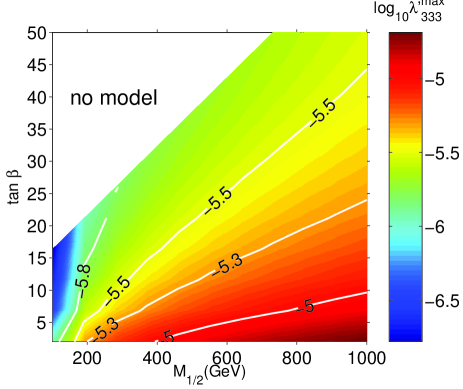
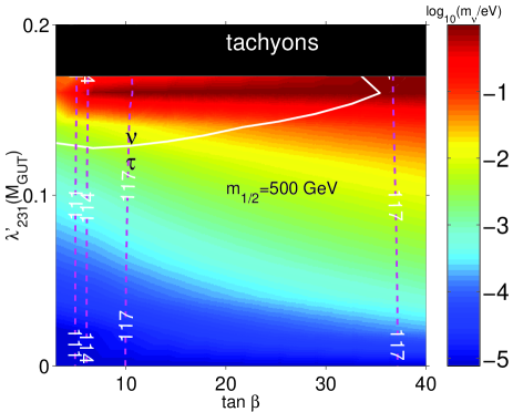
The remaining parameters ( and ) are varied in Fig. 1 and the maximum possible value of is displayed as the background colour, as referenced by the bar on the right hand side. The white region marked “no model” has tachyons for any value of and so is not valid. White contours of , , and are shown from bottom to top respectively. The strongest bound comes from the neutrino mass constraint, and we see a variation of 2 orders of magnitude on the bound across the parameter space, the strongest bounds coming from the low region. The reader should note the dependence of the neutrino mass in the simple formula Eq. (142). This strong variation of the neutrino bound is also apparent for the case of other couplings.
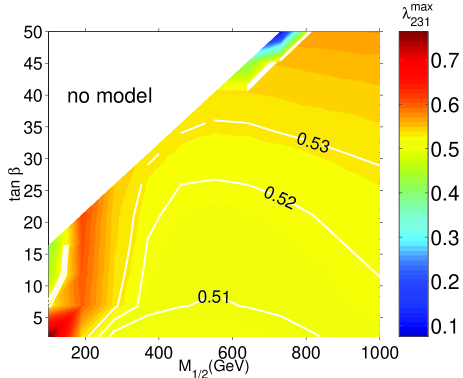
Fig. 2 shows the variation of the upper bound on with no-scale mSUGRA parameter point. The strongest bound comes from the no tachyon constraint, and we see only a small variation of the bound across the parameter space, the strongest bounds coming from the high region, at low . (Recall the sensitivity in Eq. (183).) The behaviour of small variation in the tachyon bound with supersymmetry breaking parameters is replicated for other lepton-number violating couplings. The weak bound of over much of the parameter space is dependent upon the no-charged lepton mixing at assumption.
It is instructive to compare the bounds derived here in a representative scenario of mSUGRA in Tables 3, 4 with the 2 bounds at collected in Table 1 in Ref. Allanach:1999ic for a rather generic R-parity violating scenario. For the comparison we choose the no mixing scenario, i.e. case (a) in Eqs. (175,176) and squark and slepton masses of order of 100 GeV in the latter. For the couplings, we obtain here one order of magnitude improvement for , two orders of magnitude for , three orders of magnitude for , four orders of magnitude for , five and up to six (!) orders of magnitude for . The sneutrino tachyon constraint of Eq. (183) sets slightly stronger bounds on the couplings . In the case of the -couplings we obtain two order of magnitude stronger bounds than in Ref. Allanach:1999ic for the couplings: . Sneutrino tachyons do not set better limits in this case. Comparison of the quark mixing cases (b) or (c) of Eqs. (175,176) derived in Table. 3 with the Table. IV of Ref. Allanach:1999ic show similar orders of magnitude, but stronger bounds for some of the couplings.
VII.2 LSP Content in the No-Scale Model
As outlined in the introduction, in -mSUGRA the -couplings can affect the weak-scale particle mass spectrum via the RGEs. They can also affect the interpretation of the resulting spectrum, since with the LSP is no longer stable, and thus no longer subject to cosmological constraints on stable relics. In the -mSUGRA the LSP need not be electrically and colour neutral. Before discussing the -case we briefly review the RPC case.
VII.2.1 The RPC Case
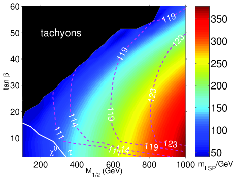
To begin with, we perform the scan in the free parameters and in R-parity conserved no-scale mSUGRA. The LSP mass and contours of equal lightest-Higgs mass are displayed in Fig. 3. The background colour displays the LSP mass according to the scale on the right hand side of the plot. The region disallowed by tachyons is shown in black. In the bottom left-hand side of the plot is a white line which shows the boundary of the LSP identity. Below the line, the LSP is the lightest neutralino, whereas above it the LSP is a right-handed stau. A charged LSP is ruled out in the R-parity conserved scenario from cosmological constraints, and so the entire region above the white line is ruled out. This bound comes from limits on abundances of anomalously heavy isotopes Ellis:1983ew . LEP2 higgs places a lower bound on the Standard Model Higgs mass of GeV. This can also be applied to the MSSM Higgs when , which is the case in all of our results. The theoretical uncertainty upon the lightest Higgs mass is estimated to be GeV Degrassi:2002fi , so we place a cautious lower bound on SOFTSUSY’s prediction of 111 GeV. Even so, we see from Fig. 3 that there is no parameter space left with both a heavy enough Higgs and a neutral LSP. Thus no-scale supergravity is ruled out for the R-parity conserved MSSM. However, even a very tiny -coupling will make the LSP unstable on cosmological time-scales and the neutral LSP constraint is then no longer applicable. For small couplings , the spectrum can be approximated by the R-parity conserved case, and so Fig. 3 can still be used. We see that the entire region above the Higgs mass contour of 111 GeV would be allowed, for stau LSP masses above 96 GeV LEP2bounds .
VII.2.2 The -Case
We now map out some parts of no-scale mSUGRA for GeV. Because we wish to show the effects of R-parity violation on the spectrum, we pick cases where the upper bound on the -trilinear coupling is weak. This obviously occurs when the tachyon bound is the stronger of the two we have shown in Tables 3 and 4. We display one -type coupling (Fig 4), one of type (Fig 5) and one of type (Fig 6).
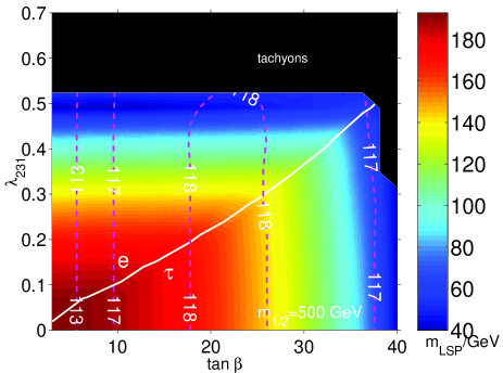
Fig. 4 shows the variation of the nature of the LSP with and . The case (b) of Eqs. (175,176) is considered. For GeV, as assumed here, we see from the equal Higgs mass contours, that the lower bound of 111 GeV on the lightest-Higgs mass does not pose a very severe constraint for . The LSP mass varies up to 190 GeV in the plane, but this value is a function of . The diagonal white line separates regions of selectron LSP (above the white line) and stau LSP (below the white line). Note that there is an independent (2) bound for the coupling from the known ratios corresponding to Allanach:1999ic ; Han : . Comparing this bound with the nature of the LSP in Fig. 4 we observe that the scalar tau LSP is favoured for unless the above laboratory bound is evaded by taking .
In Fig. 5, we show the variation of the non-zero neutrino mass in the plane. Neutrino masses provide the upper bound upon for mixing in the up-quark sector [case (c) in Eqs. (175,176)], as assumed here. For larger values of , neutrino masses of are possible. In this case, above the white line, the LSP is a tau sneutrino, and below it the LSP is the stau. The laboratory bound for the coupling reads Allanach:1999ic ; Han : and since we find that for the inputs of Fig. 5 the bottom squark mass is about 1.2 TeV, the laboratory bound is evaded: the stronger bound on comes from the sneutrino tachyon as is shown in the upper half of Fig. 5.
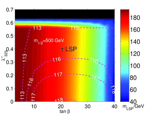
Finally, we investigate the case of baryon number violation. The case (b) of Eqs. (175,176) is considered. Fig. 6 shows how the no-scale mSUGRA LSP mass varies with and . There is little variation with the -coupling, contrary to the lightest Higgs mass, which is displayed in the form of contours. The previous bound on (see Table IV of bound Allanach:1999ic ) apart from the theoretical perturbativity bound comes from the leptonic Z-width ratio and is for quark mixing solely in the down-quark sector, and with a little variation from . We observe from Fig. 6 that the stau is again the LSP.
We have exhibited, in Figs. 3-6, viable regions of MSSM parameter space where the LSP is the selectron, the stau or the stau sneutrino. Different LSP content drastically alters the collider signatures of the models. The analysis above showed a preference to the stau being the LSP. We discuss this in some more detail in Sect. VIII, below.
VII.3 Sneutrino-Antisneutrino Mixing with Stau LSP
Models which violate lepton number by two units () and generate neutrino masses, also result in a mass splitting of scalar neutrinos and anti-neutrinos of the same flavour usually referred in the literature as sneutrino anti-sneutrino mixing HG1 ; Hirsch ; Chun2 . If the sneutrino mass difference , is large and the sneutrino branching ratio into a charged lepton is experimentally significant, then a like sign-dilepton signal in with could be observed HG1 . Like the B-meson mass splitting , the observability of the sneutrino mixing effects depend on the ratio
| (184) |
where is the total sneutrino decay rate. As we have already seen from Figs. 4-6, in the no-scale scenario the stau, , is the LSP when the -couplings are small. In this (approximately RPC) case the specific flavour sneutrino decays, via charginos and neutralinos into and . In this case, the probability of tagging a like-sign dilepton in the process is with HG1
| (185) |
We investigate below the magnitude of this probability in the no-scale model with GeV and and with one dominant -coupling . Furthermore we consider no-quark mixing in determining the relevant bounds from the neutrino masses. In this model the stau is the LSP. We first calculate the sneutrino mass squared difference
| (186) |
where is the average mass of . The sneutrino mass difference has been calculated in Ref. HG2 in a general basis independent manner. With our choice we generate at the electroweak scale the non-zero -parameter set: . The other -parameters remain zero footx . This simplifies our calculation for the sneutrino mass splitting, since we can use the case of one sneutrino generation (the other two decouple from the mass matrices Eqs. (82,89)). The sneutrino mass splitting reads HG2 :
| (187) |
with
| (188) |
Notice that Eq. (187) does not depend on the superpotential parameters in contrast to the neutrino mass in Eq. (140). It is helpful to see the numerical values footy for the parameters at the electroweak scale starting from the no-scale model defined by: GeV, and . We obtain: , GeV, GeV, GeV, GeV, GeV, GeV, , and . Applying these values to Eqs. (187,188) we obtain and eV. The sneutrino mass splitting is of the same order as the neutrino mass obtained from Eq. (140), since for GeV and GeV we have eV footz .
In order to calculate the probability we still need the total sneutrino decay rate and the branching ratio . In the above scenario the right handed selectron of the third generation (we call it stau here although it is in fact an admixture of the three charged sleptons with the charged Higgs boson states) is the LSP with a mass GeV. The rates for the chargino and neutralino mediated sneutrino decays (which we assume to be the dominant ones) are HG1 :
| (189) |
with
| (190) |
In the no-scale model under consideration we obtain: GeV, GeV with the gauge couplings and . Thus from Eq. (189) we obtain: eV and eV. So and . We conclude that in this numerical example the probability for like sign dileptons, Eq. (185), is: , far too small to be observable. Of course this result depends on the parameter space and the probability is bigger for smaller values of and larger values (see Eq. (189). However, if we take into account the current experimental data, , then . We obtain similar results for the other -couplings.
The above benchmark computation can be helpful to the reader in order understand the typical magnitude of the parameters we are dealing with in this paper.
VIII Stau-LSP Phenomenology
As discussed in Sect. I, in the case of , the LSP need not be the lightest neutralino, . In the previous section we have investigated the nature of the LSP in the mSUGRA scenario and have found regions in parameter space with different LSP’s. In Fig. 4, we have a selectron or stau LSP, in Fig. 5 we have found a tau sneutrino or a stau and in Fig. 6 we have found a stau LSP. The bounds in Table 3 imply that if there is any appreciable CKM mixing in the down-quark sector at the weak scale, must be very small. We also see some strict bounds upon the in Table 4. If the -couplings are very small, the spectrum has negligible perturbation from the R-parity conserved case, the LSP content of which is displayed in Fig. 3. The allowed parameter space with in Fig. 3 then leads to a stau LSP. Thus we see a preference for a stau LSP in many no-scale R-parity violating scenarios.
In the RPC-MSSM, the collider phenomenology relies crucially on the -LSP, with all produced sparticles decaying in the detector to plus other -even particles. This results in missing transverse energy as a typical signature for all production processes. In the -MSSM the RGEs and thus the spectrum, is altered. This changes the decay chains. Since typically all decay chains end in the LSP, the nature of the LSP is essential in determining the supersymmetric signatures. A detailed investigation is beyond the scope of this paper. We shall here focus on a classification of the signatures for the main production processes in the case of a stau LSP.
VIII.0.1 Stau Decays
The following discussion of the stau-LSP is somewhat analogous to the discussion in Ref. Dreiner:pe for the -LSP. In determining the final state signature it is important to know how the stau-LSP decays. We shall assume that there is a hierarchy among the -coupling constants with one dominant coupling, similar to the SM Yukawa couplings in the mass eigenstate basis. We furthermore assume the mixing due to is small as seen in the previous sections of this paper. Then there are two important distinct cases.
-
1.
The stau couples to the dominant operator. The dominant operator is in the set . In this case, the stau simply decays via the two-body mode. For the dominant operator for example we then obtain Dreiner:1999qz
(191) where is the number of colours. The complete list of , two-body decays is given in Ref. Dreiner:1999qz . For a recent treatment of two-body stau decays also see Porod . For the above two-body decay mode the decay length is given by
(192) which in an experiment must be multiplied by the relevant Lorentz boost factor of the stau. Only for very small coupling () is the decay length relevant.
-
2.
The stau doesn’t couple to the dominant operator. The dominant operator is in the set . In this case the decays via a four-body mode. For the operator there are four decay modes via the neutralino
(193) and three decay modes via the chargino
(194) As an example we here compute the decay . The details of the computation, in particular the four-body phase space are given in Appendix D. The result is
(195) where . are neutralino coupling constants given in the appendix. is the neutralino mass and is the universal scalar fermion mass. We have assumed massless final state particles and neglected the momenta compared to . In the last step we have set the couplings , the weak coupling constant. If the four-body decay is the dominant decay mode, the decay length can be estimated as
(196) For reasonable supersymmetric masses and couplings this could lead to detached vertices in the detector. This is a very promising signature for the stau-LSP.
If the two-body decay is allowed, i.e. the relevant coupling is not suppressed, it usually dominate over the four-body decay. In order to estimate the required hierarchy of couplings for the four-body decay to be relevant we consider the ratio
| (197) |
Assuming the sparticle masses are roughly equal, this corresponds to for the 4-body decay mode to dominate over the 2-body one. If, for example, , we obtain , which is not an unreasonable hierarchy between generations.
VIII.0.2 Collider Signatures
At a collider, the main supersymmetric pair production processes are
| (198) |
Here we investigate the possible signatures for these processes in the case of a stau LSP. In order to determine the final state within the detector, we must know the decay patterns of the particles. This strongly depends on the supersymmetric spectrum and thus upon which point in SUSY breaking parameter space is being studied. For this first study, we shall assume the mass ordering
| (199) |
which we typically obtain (with or without ) within mSUGRA. If there are no near-degenerate particles, a produced supersymmetric particle will dominantly cascade in two-particle decays down the mass chain (199). We display this decay chain in Fig. 7. We have added at the end both two- (in red) and four-particle (in blue) stau decays. Final state quarks are denoted by “j” to indicate a jet.
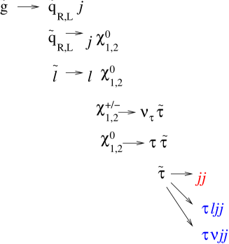
We can use this decay chain to determine a qualitative picture of the possible final state signatures. Note that due to the strict bounds on the -couplings which we have determined we only expect these to be relevant in the stau-LSP decay. Furthermore, in determining signatures we shall assume that either the two-body or the four-body stau decay dominates. We do not consider the case of comparable partial decay widths.
At the Tevatron and LHC the largest production cross sections are for gluinos and squarks. If we consider for example production, then the dominant decay mode for the squark is
| (200) |
and the final state signature will be
| (201) |
Here, any charge combination for the leptons is allowed, since they result from the decay of a virtual (Majorana) neutralino (c.f. App. D). This can give us a like-sign di-lepton signature. Otherwise, we see that we have a large number of jets in the final state independent of the decay mode of the stau. (This would be reduced for dominant operators .) This makes it more difficult to observe isolated high charged leptons. We can obtain missing transverse momentum from the final state neutrinos but it will be extremely diluted due to the many body-decays. The most promising signature are like-sign dileptons together with the direct detection of ’s tau-signat , which is of course difficult.
For -production, we expect a larger liklihood for the cascade decay through the heavier neutralinos and also through the charginos. This can lead to a tri-lepton signature trilepton which can be extended by the additional ’s. This requires a detailed analysis but we expect this to be more promising than the outlined above.
The gluino decays via the squarks adding an extra jet to the final state. In this case it might be more promising to consider non-dominant decay modes, including a possible direct -decay of the neutralino. An estimate of the relative rates for a pure wino neutralino is
| (202) |
for , and where we have neglected the stau mass. This is hopeless, unless the neutralino and the stau are nearly degenerate.
At the Tevatron and LHC the pair production of sleptons is about two to three orders of magnitude lower than the production of squarks or gluinos, for equal mass. However, we expect the mass to be lower (c.f. Eq.(199)), and also the signal cleaner. At a future linear collider facility this is typically an ideal mode for searches or the measurement of MSSM parameters. As we can see from the decay chain in Fig. 7, the slepton dominantly decays as
| (203) |
We then obtain the final-state signatures
| (204) |
In the second case the sign of the charge of the two leptons from the stau decays is arbitrary due to the intermediate (Majorana) neutralino. Thus we can have like-sign tri-leptons, which is a very promising signature.
Similarly, using the results from Fig. 7, we expect the as dominant signatures for neutralino pair production
| (205) |
depending on the decay of the stau-LSP decay which in turn depends on the dominant -coupling. For chargino pair production we have
| (206) |
assuming the chargino decays directly to the stau LSP. If we produce the heavier electroweak gauginos we can cascade decay through the lighter gauginos producing more charged leptons. For the neutralino we have promising multi-lepton sigantures, whereas for the chargino we expect a significant amount of missing .
In summary, as promising signatures in the case of the stau LSP we have
-
1.
A detached vertex from the long lived stau, particularly in the case of the four-body stau decay.
-
2.
Multilepton final states.
-
3.
Multi-tau final states, requiring efficient tau tagging.
The four-body decay of the stau results in more final state leptons than the two-body decay and is thus possibly more promising.
IX Summary and Conclusions
We have investigated for the first time the general -MSSM in the context of mSUGRA. We have studied in some detail the origin of lepton-number violation and have found that with respect to the dimension-five operators baryon-parity is preferred over R-parity. We have then shown that in a wide class of models both and are zero after supersymmetry breaking at the unification scale. We have taken this as our boundary conditions at in order to investigate the resulting model in considerable detail.
In order to embed the model within the unification picture we have computed the full set of renormalzation group equations in the appendices. We have used two methods, including a novel method of Jones et al., which is particularly conducive to the numerical implementation. We then developed an iterative algorithm which solves the RGEs, minimises the potentail of the five neutral, scalar, CP-even fields, while implementing weak-scale Yukawa and gauge boundary conditions. The algorithm is stable and has been checked by an independent program. This is one of the main technical advances in this paper. Given the minimum, we determined the complete supersymmetric spectrum, including also the mass of the heaviest neutrino.
We have then shown that the -couplings in this model are severely constrained by the upper bound on the neutrino masses, as summarized in Tables 3 and 4. Thus when embedding the -MSSM in mSUGRA the neutrino mass bound is the strictest and most universal, i.e. applies to all lepton number violating couplings. This is one of the main results of this paper.
We have then looked in detail at the nature of the LSP. We have found solutions with a selectron, tau sneutrino and stau LSP besides the usual neutralino LSP, with the stau most favoured in the noscale mSUGRA model. This significantly affects collider phenomenology. We present a first discussion of this broad topic in Sect. VIII. We have also studied the phenomenology of sneutrino-antisneutrino mixing in this model, but do not expect any significant effect.
We conclude that the -MSSM is as viable as the RPC-MSSM. As we show, it considerably differs both conceptually and phenomenologically from the RPC. The intimate connection with neutrino masses is an outstanding feature which we shall discuss in more detail in a forthcoming publication.
Acknowledgments
We would like to thank I Jack, D R T Jones and A F Kord for helping to bring an error in eq. (86) to our attention in a previous version of thie paper, and for graciously collaborating on detailed numerical comparisons jj . HKD would like to thank Goran Senjanovic for discussions on GUTs and R-parity violation and Howie Haber for discussions on the integration of four-particle phase space. AD would like to thank M. Drees for useful discussions on the WMAP neutrino bound. AD and HKD would like to thank the CERN theory division for hospitality offered while some of this work was performed. BCA would like to thank the University of Bonn for hospitality offered while some of the work contained herein was carried out. We also thank S Rimmer for help with a conventions check. AD acknowledges support in part by the German Bundesministerium für Bildung und Forschung under the contract 05HT1WOA3 and the ‘Deutsche Forschungsgemeinschaft’ DFG Project Bu. 706/1-2.
Appendix A Notation and Anomalous Dimensions
The chiral superfields of the -MSSM and the -MSSM have the following quantum numbers
| (207) |
The -MSSM superpotential is then given by
| (208) | |||||
We denote an colour index of the fundamental representation by . The fundamental representation indices are denoted by and the generation indices by . We have introduced the twelve matrices
| (209) |
for all the Yukawa couplings. This implies the following conventions in the Martin and Vaughn mv notation
| (210) | |||||
| (211) | |||||
| (212) |
The soft SUSY breaking Lagrangian is given by,
| (213) | |||||
where we have introduced the soft SUSY breaking trilinear couplings
| (214) |
In general the one-loop renormalization group equations for the Yukawa couplings are given by mv
| (215) |
and the anomalous dimensions are
| (216) |
We have denoted by the quadratic Casimir of the representation of the gauge group . For details see the Appendix A of Ref. add . All equations in this section are valid in the renormalisation scheme.
The one-loop anomalous dimensions are given by add ; typo :
| (217) | |||||
| (218) | |||||
| (219) | |||||
| (220) | |||||
| (221) | |||||
| (222) | |||||
| (223) | |||||
| (224) |
Note that here, represent the fields , , where is the index of the fundamental representation of (i.e. no factors of are factored). The -functions for the Yukawa couplings add and for the bilinear superpotential couplings are combinations of the above anomalous dimensions (217-224). The two loop anomalous dimensions in the -MSSM can be found in add . We present the one-loop beta functions for the superpotential couplings and masses for completeness.
The RGEs for the Yukawa couplings (including full family dependence) are given by
| (225) | |||||
| (226) | |||||
| (227) | |||||
| (228) | |||||
| (229) | |||||
| (230) |
Here , and is the renormalization scale. The RGEs for the bilinear terms are
| (231) | |||||
| (232) |
Appendix B A method to derive the soft SUSY breaking RGEs
A straightforward way to derive the RGEs for the soft SUSY breaking couplings and masses is by a direct use of the explicit formulæ at 1-loop given in mv . This is a somewhat tedious job. A very elegant method which is also very helpful for numerical calculations is the one described in Ref. jones . All the soft SUSY RGEs can be derived from the anomalous dimensions (217-224) by the action of an operator which is given below gauginomasses . The method works not only at one loop but it has been proven to all orders in perturbation theory jones . In principle one could apply the operators (B1-B5) below to the 2-loop anomalous dimensions derived in Ref. add and write down the full two loop coupled RGEs in the most general case. However, here we restrict ourselves to the one-loop case. In particular the soft -functions for the bilinear , trilinear and scalar masses soft SUSY breaking terms can be read from
| (233) | |||||
| (234) | |||||
| (235) |
where
| (236) | |||||
| (237) |
and repeated indices are summed over. At one loop the last term, ,in Eq. (235) is not relevant. Its (scheme dependent form) is given for example in the last reference of Ref. jones (see their Eq. (2.11)). The RGEs (233-235) are valid as long as we do not eliminate the U(1) Fayet-Iliopoulos (FI) D-term. The RGE running of the FI-term can then be written independently. It is known that for universal boundary conditions this term is not renormalized down to low energies and we do not discuss its RGE here. On the other hand if we eliminate the FI D-term by using its equation of motion then this renormalization gives rise to additional contributions proportional to the U(1) gauge coupling (see the -term in the RGEs for the soft SUSY breaking masses in the Appendix C). Now from Eq. (233) the RGEs for the bilinear soft SUSY breaking masses in the -MSSM are
| (238) | |||||
| (239) |
The RGEs for the trilinear soft SUSY breaking masses in the -MSSM can be read from Eq. (234)
| (240) | |||||
| (241) | |||||
| (242) | |||||
| (243) | |||||
| (244) | |||||
| (245) | |||||
The RGEs for the soft SUSY breaking masses in the -MSSM can be obtained from Eq. (235)
| (246) | |||||
| (247) | |||||
| (248) | |||||
| (249) | |||||
| (250) | |||||
| (251) | |||||
| (252) | |||||
| (253) | |||||
where from Eq. (236) we have
| (254) | |||||
| (255) | |||||
| (256) | |||||
| (257) | |||||
| (258) | |||||
| (259) | |||||
| (260) | |||||
| (261) |
and from Eq. (237)
| (262) | |||||
| (263) | |||||
| (264) | |||||
| (265) | |||||
| (266) | |||||
| (267) |
Numerically we follow the following procedure :
- (a)
- (b)
- (c)
- (d)
This is much simpler than inserting the explicit formulæ of Appendix C below.
Appendix C Explicit RGEs for the soft supersymmetric breaking terms
The explicit RGEs for the soft supersymmetric breaking terms have appeared also before in Refs.deCarlos:1996du and Besmer:2000rj . Ref.Besmer:2000rj contains the full set (aside from the aforementioned term), but we disagree with several terms in the equations for and . Ref. deCarlos:1996du is restricted to contributions of the third generation quarks and leptons. We arrange here the explicit formulæ of the full (not flavour dominance assumed) RGEs. As a cross check, we have calculated them by first using the explicit formulae of Ref. mv and second by using the method described in Appendix B. We found agreement using both methods. Thus the RGE for the bilinear and terms of the superpotential parameters is given by
| (268) | |||||
| (269) | |||||
Similarly, the RGEs for the soft SUSY breaking bilinear terms can be read from,
| (270) | |||||
| (271) | |||||
The RGEs for the soft SUSY trilinear couplings are given by
| (272) | |||||
| (273) | |||||
| (274) | |||||
| (275) | |||||
| (276) | |||||
| (277) | |||||
The RGEs for the gaugino masses are not affected by the -couplings up to 1-loop. The RGEs for the SUSY soft breaking masses are given by,
| (278) | |||||
| (279) | |||||
| (280) | |||||
| (281) | |||||
| (282) | |||||
| (283) | |||||
| (284) | |||||
| (285) | |||||
where
| (286) |
and
| (287) |
Appendix D Four-Body -Decay
In this Appendix we compute the four-body decay via the -operator . The relevant Feynman diagrams are given in Fig. 8 a,b,c. We neglect the contributions from the heavier neutralinos. Using the notation of Ref. Peter the three amplitudes corresponding to Fig. 8 are given by:
| (288) | |||||
| (289) | |||||
| (290) |
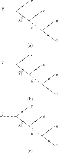
Here the four-momenta are denoted by the particle symbol. The momenta flow along the corresponding propagators from left to right. We use below that as well as the notation for the denominators in the propagators. We have assumed there is no mixing in the scalar and sectors. However, we allow for mixing in the stau sector. , , are the only sparticles that couple to the R-parity violating operators. The coupling constants are given by Kane ; Haber ; Peter
| (291) | |||||
| (292) | |||||
| (293) |
The total matrix element squared is given by
| (294) |
where is the colour factor and
| (295) | |||||
| (296) | |||||
| (297) | |||||
| (298) | |||||
| (299) | |||||
| (300) |
The functions are given by
| (301) |
The squared amplitude in Eq.(294) can be used in Monte Carlo simulation programs to generate events with a decaying stau. We are here interested in an analytic approximation for the total decay width. To this end, we shall assume . This is equivalent above to setting . Furthermore we assume that all scalar propagators are dominated by their mass terms and the scalar fermion mass is universal: . In this simplified case the amplitude squared is given by
The total width is given by Howie ; Singh
| (303) |
where . After the simplification our matrix element squared consists of three kinds of terms which depend on the final state four-momenta: and . As can be seen from the phase space integral, these all contribute the same, they simply correspond to a relabeling. We thus explicitly integrate only the first term. Using Eq (4) from Ref. Howie with , we see that
| (304) |
and we thus obtain
| (305) |
In the rest-frame of the decaying stau with the z-axis in the direction of the 3-momentum of the
| (306) |
Performing the integrals over and
| (307) |
It is convenient to change to dimensionless variables and Howie . Implementing the integral boundaries given in Refs. Singh ; Howie , this leads to the result
| (308) |
We thus have for the total width
| (309) |
where .
References
- (1) H. P. Nilles, Phys. Rept. 110 (1984) 1.
- (2) H. E. Haber and G. L. Kane, Phys. Rept. 117, 75 (1985).
- (3) S. P. Martin, arXiv:hep-ph/9709356.
- (4) U. Amaldi, W. de Boer and H. Furstenau, Phys. Lett. B 260 (1991) 447; J. R. Ellis, S. Kelley and D. V. Nanopoulos, Nucl. Phys. B 373, 55 (1992); P. Langacker and N. Polonsky, Phys. Rev. D 47, 4028 (1993) [arXiv:hep-ph/9210235]; for a detailed technical treatment of the unification constraints see for example A. Dedes, A. B. Lahanas and K. Tamvakis, Phys. Rev. D 53 (1996) 3793 [arXiv:hep-ph/9504239].
- (5) The cases of gauge-mediated and anomaly mediated supersymmetry breaking are not discussed here.
- (6) R. Hempfling, Nucl. Phys. B 478 (1996) 3 [arXiv:hep-ph/9511288].
- (7) M. Hirsch, M. A. Diaz, W. Porod, J. C. Romao and J. W. Valle, Phys. Rev. D 62 (2000) 113008 [Erratum-ibid. D 65 (2002) 119901] [arXiv:hep-ph/0004115].
- (8) B. de Carlos and P. L. White, Phys. Rev. D 54 (1996) 3427 [arXiv:hep-ph/9602381].
- (9) B. de Carlos and P. L. White, Phys. Rev. D 55, 4222 (1997) [arXiv:hep-ph/9609443].
- (10) P. Fayet, Phys. Lett. B 69 (1977) 489. G. R. Farrar and P. Fayet, Phys. Lett. B 76, 575 (1978).
- (11) S. Weinberg, Phys. Rev. D 26 (1982) 287. Phenomenology of the terms , and in (4) were first considered in L. J. Hall and M. Suzuki, Nucl. Phys. B 231 (1984) 419. Phenomenology of the term in the superpotential (4) was first considered in F. Zwirner, Phys. Lett. B 132 (1983) 103.
- (12) H. K. Dreiner, arXiv:hep-ph/9707435.
- (13) A. Y. Smirnov and F. Vissani, Nucl. Phys. B 460 (1996) 37 [arXiv:hep-ph/9506416].
- (14) B. C. Allanach, A. Dedes and H. K. Dreiner, Phys. Rev. D 60, 056002 (1999) [arXiv:hep-ph/9902251].
- (15) I. Jack, D. R. Jones and A. Pickering, Phys. Lett. B 426, 73 (1998) [arXiv:hep-ph/9712542]; L. V. Avdeev, D. I. Kazakov and I. N. Kondrashuk, Nucl. Phys. B 510, 289 (1998) [arXiv:hep-ph/9709397]; I. Jack and D. R. Jones, Phys. Lett. B 415, 383 (1997) [arXiv:hep-ph/9709364]; I. Jack, D. R. Jones and A. Pickering, Phys. Lett. B 432, 114 (1998) [arXiv:hep-ph/9803405]; I. Jack and D. R. Jones, Phys. Lett. B 465, 148 (1999) [arXiv:hep-ph/9907255].
- (16) S. P. Martin and M. T. Vaughn, Phys. Rev. D 50, 2282 (1994) [arXiv:hep-ph/9311340]; Y. Yamada, Phys. Rev. D 50, 3537 (1994) [arXiv:hep-ph/9401241]; I. Jack and D. R. Jones, Phys. Lett. B 333, 372 (1994) [arXiv:hep-ph/9405233]; I. Jack, D. R. Jones, S. P. Martin, M. T. Vaughn and Y. Yamada, Phys. Rev. D 50, 5481 (1994) [arXiv:hep-ph/9407291].
- (17) V. D. Barger, M. S. Berger, R. J. Phillips and T. Wohrmann, Phys. Rev. D 53 (1996) 6407 [arXiv:hep-ph/9511473].
- (18) B. C. Allanach, A. Dedes and H. K. Dreiner, Phys. Rev. D 60 (1999) 075014 [arXiv:hep-ph/9906209].
- (19) G. Bhattacharyya, Nucl. Phys. Proc. Suppl. 52A (1997) 83 [arXiv:hep-ph/9608415].
- (20) L. E. Ibanez and G. G. Ross, Nucl. Phys. B 368 (1992) 3; L. E. Ibanez and G. G. Ross, Phys. Lett. B 260 (1991) 291. On discrete gauge symmetries that forbid proton decay but contain an additional singlet superfield see: S. Lola and G. G. Ross, Phys. Lett. B 314 (1993) 336; and for an additional quark isosinglet (-1/3) see D. J. Castano and S. P. Martin, Phys. Lett. B 340 (1994) 67 [arXiv:hep-ph/9408230].
- (21) L. E. Ibanez and G. G. Ross, Phys. Lett. B110 (1982) 215; K. Inoue, A. Kakuto, H. Komatsu and S. Takeshita, Prog. Theor. Phys. 68, 927 (1982) and Erratum, ibid. 70 (1983) 330; Prog. Theor. Phys. 71 (1984) 413; L. Alvarez-Gaumé, M. Claudson and M. B. Wise, Nucl. Phys. B207 (1982) 96; J. R. Ellis, J. S. Hagelin, D. V. Nanopoulos and K. Tamvakis, Phys. Lett. B125 (1983) 275.
- (22) H. K. Dreiner and H. Pois, arXiv:hep-ph/9511444.
- (23) E. Nardi, Phys. Rev. D 55 (1997) 5772 [arXiv:hep-ph/9610540].
- (24) L. J. Hall and M. Suzuki in Ref. Weinberg81 .
- (25) J. R. Ellis, G. Gelmini, C. Jarlskog, G. G. Ross and J. W. Valle, Phys. Lett. B 150 (1985) 142.
- (26) T. Banks, Y. Grossman, E. Nardi and Y. Nir, Phys. Rev. D 52 (1995) 5319 [arXiv:hep-ph/9505248].
- (27) D. N. Spergel et al., arXiv:astro-ph/0302209.
- (28) M. Colless et al., arXiv:astro-ph/0306581.
- (29) B. W. Lee and S. Weinberg, Phys. Rev. Lett. 39 (1977) 165.
- (30) H. Goldberg, Phys. Rev. Lett. 50 (1983) 1419.
- (31) J. R. Ellis, J. S. Hagelin, D. V. Nanopoulos, K. A. Olive and M. Srednicki, Nucl. Phys. B 238 (1984) 453; P.F. Smith et al, Nucl. Phys. B 206 333 (1982).
- (32) However, observational bounds on long-lived particles must be taken into account Ellis:1990nb .
- (33) J. R. Ellis, G. B. Gelmini, J. L. Lopez, D. V. Nanopoulos and S. Sarkar, Nucl. Phys. B 373 (1992) 399.
- (34) H. K. Dreiner and G. G. Ross, Nucl. Phys. B 365 (1991) 597; B. Allanach et al., arXiv:hep-ph/9906224.
- (35) A. G. Akeroyd, M. A. Diaz, J. Ferrandis, M. A. Garcia-Jareno and J. W. Valle, Nucl. Phys. B 529 (1998) 3 [arXiv:hep-ph/9707395].
- (36) A. G. Akeroyd, C. Liu and J. Song, Phys. Rev. D 65 (2002) 015008 [arXiv:hep-ph/0107218].
- (37) A. Bartl, M. Hirsch, T. Kernreiter, W. Porod and J. W. Valle, arXiv:hep-ph/0306071.
- (38) M. Hirsch and W. Porod, arXiv:hep-ph/0307364.
- (39) A. de Gouvea, A. Friedland and H. Murayama, Phys. Rev. D 59 (1999) 095008 [arXiv:hep-ph/9803481].
- (40) H. Baer, K. m. Cheung and J. F. Gunion, Phys. Rev. D 59 (1999) 075002 [arXiv:hep-ph/9806361]; S. Raby and K. Tobe, Nucl. Phys. B 539 (1999) 3 [arXiv:hep-ph/9807281]. A. Mafi and S. Raby, Phys. Rev. D 62 (2000) 035003 [arXiv:hep-ph/9912436].
- (41) M. C. Bento, L. J. Hall and G. G. Ross, Nucl. Phys. B 292 (1987) 400.
- (42) L. M. Krauss and F. Wilczek, Phys. Rev. Lett. 62 (1989) 1221.
- (43) T. Banks and M. Dine, Phys. Rev. D 45 (1992) 1424 [arXiv:hep-th/9109045].
- (44) Here we use the notation of Ref. Ibanez:1991pr .
- (45) From Table 2, it is obvious that the model contains the infamous non-renormalizable neutrino mass term which gives rise to neutrino masses of order of eV if the cut-off is bigger than GeV. In deriving the bounds on the couplings and we shall assume that neutrino masses arising from this operator are much smaller than 1 eV . In any case, the addition of the term is needed when trying to make a detailed analysis of the neutrino spectrum..
- (46) D. E. Brahm and L. J. Hall, Phys. Rev. D 40 (1989) 2449. For a flipped- version with and , -operators see K. Tamvakis, Phys. Lett. B 382 (1996) 251 [arXiv:hep-ph/9604343].
- (47) K. Tamvakis, Phys. Lett. B 383 (1996) 307 [arXiv:hep-ph/9602389].
- (48) H. Fritzsch and P. Minkowski, Annals Phys. 93 (1975) 193.
- (49) C. S. Aulakh, B. Bajc, A. Melfo, A. Rasin and G. Senjanovic, Nucl. Phys. B 597 (2001) 89 [arXiv:hep-ph/0004031]; C. S. Aulakh, A. Melfo, A. Rasin and G. Senjanovic, Phys. Lett. B 459 (1999) 557 [arXiv:hep-ph/9902409]; D. G. Lee and R. N. Mohapatra, Phys. Rev. D 51 (1995) 1353 [arXiv:hep-ph/9406328].
- (50) G. F. Giudice and R. Rattazzi, Phys. Lett. B 406 (1997) 321 [arXiv:hep-ph/9704339].
- (51) A. E. Faraggi, Phys. Lett. B 398 (1997) 95 [arXiv:hep-ph/9612400]; W. Pokorski and G. G. Ross, Nucl. Phys. B 551 (1999) 515 [arXiv:hep-ph/9809537].
- (52) H. Dreiner and M. Thormeier, hep-ph/0305270.
- (53) See page 182-183 of S. Weinberg, “The Quantum Theory Of Fields. Vol. 3: Supersymmetry,” Cambridge, UK: Univ. Pr. (2000) 419 p.
- (54) For a more extensive discussion of R-symmetries including lepton-number violation see for example Chamseddine:1995gb .
- (55) A. H. Chamseddine and H. Dreiner, Nucl. Phys. B 458 (1996) 65 [arXiv:hep-ph/9504337].
- (56) Lepton flavour can still be violated, e.g. through a combination of terms for example. The process via resonant squark production Butterworth:tc does not violate this lepton number since the chargino carries lepton number.
- (57) J. Butterworth and H. K. Dreiner, Nucl. Phys. B 397 (1993) 3 [arXiv:hep-ph/9211204].
- (58) J. E. Kim and H. P. Nilles, Phys. Lett. B 138 (1984) 150.
- (59) G. F. Giudice and A. Masiero, Phys. Lett. B 206 (1988) 480.
- (60) E. J. Chun, J. E. Kim and H. P. Nilles, Nucl. Phys. B 370 (1992) 105. J. A. Casas and C. Munoz, Phys. Lett. B 306 (1993) 288 [arXiv:hep-ph/9302227]. Y. Nir, Phys. Lett. B 354 (1995) 107 [arXiv:hep-ph/9504312]. A. H. Chamseddine and H. K. Dreiner, Phys. Lett. B 389 (1996) 533 [arXiv:hep-ph/9607261]. H. P. Nilles and N. Polonsky, Nucl. Phys. B 484 (1997) 33 [arXiv:hep-ph/9606388].
- (61) We follow here the notation and discussion in Soni:1983rm .
- (62) S. K. Soni and H. A. Weldon, Phys. Lett. B 126 (1983) 215.
- (63) H. P. Nilles, Phys. Lett. B 115 (1982) 193.
- (64) R. D. Peccei and H. R. Quinn, Phys. Rev. Lett. 38 (1977) 1440.
- (65) See for example, p.25 in Ref. Martin:1997ns
- (66) Y. Grossman and H. E. Haber, Phys. Rev. D 59, 093008 (1999) [arXiv:hep-ph/9810536].
- (67) For the one loop corrections to the effective potential in the MSSM+ see E. J. Chun and S. K. Kang, Phys. Rev. D 61 (2000) 075012 [arXiv:hep-ph/9909429]; S. Davidson, M. Losada and N. Rius, Nucl. Phys. B 587 (2000) 118 [arXiv:hep-ph/9911317]. Dominant two loop corrections to the minimization conditions of the MSSM with R-parity symmetry, have recently been computed by A. Dedes and P. Slavich in Ref. Dedes:2002dy .
- (68) M. Nowakowski and A. Pilaftsis, Nucl. Phys. B 461 (1996) 19 [arXiv:hep-ph/9508271].
- (69) A. Dedes and P. Slavich, Nucl. Phys. B 657 (2003) 333 [arXiv:hep-ph/0212132].
- (70) We have corrected the sign error for the parameter in Eq. (3.2) of Ref. Haber . We would like to thank H. Haber for communication.
- (71) When the SUSY GUT relation is dropped an arbitrarily light neutralino is still allowed by collider experiments light-LSP ; supernova , although constrained by cosmology cosmo ; supernova .
- (72) D. Choudhury, H. K. Dreiner, P. Richardson and S. Sarkar, Phys. Rev. D 61 (2000) 095009 [arXiv:hep-ph/9911365].
- (73) H. Dreiner, C. Hanhart, U. Langenfeld and D. R. Phillips, arXiv:hep-ph/0304289.
- (74) D. Hooper and T. Plehn, Phys. Lett. B 562 (2003) 18 [arXiv:hep-ph/0212226]; A. Bottino, N. Fornengo and S. Scopel, Phys. Rev. D 67 (2003) 063519 [arXiv:hep-ph/0212379].
- (75) A. S. Joshipura and M. Nowakowski, Phys. Rev. D 51, 2421 (1995) [arXiv:hep-ph/9408224].
- (76) We use the notation .
- (77) J. R. Ellis, A. B. Lahanas, D. V. Nanopoulos and K. Tamvakis, Phys. Lett. B 134 (1984) 429; J. R. Ellis, C. Kounnas and D. V. Nanopoulos, Phys. Lett. B 143, 410 (1984); J. R. Ellis, K. Enqvist and D. V. Nanopoulos, Phys. Lett. B 147, 99 (1984). For a review, A. B. Lahanas and D. V. Nanopoulos, Phys. Rept. 145, 1 (1987), and references therein.
- (78) See for example, p.50-55 in Ref. Martin:1997ns . For R-parity violating gauge mediated supersymmetry breaking (GMSB) see: E. J. Chun, Phys. Lett. B 454 (1999) 304 [arXiv:hep-ph/9901220];
- (79) L. Randall and R. Sundrum, Nucl. Phys. B 557 (1999) 79 [arXiv:hep-th/9810155]. For R-parity violating anomaly mediated supersymmetry breaking (AMSB) see: B. C. Allanach and A. Dedes, JHEP 0006 (2000) 017 [arXiv:hep-ph/0003222]; F. De Campos, M. A. Diaz, O. J. Eboli, M. B. Magro and P. G. Mercadante, Nucl. Phys. B 623 (2002) 47 [arXiv:hep-ph/0110049].
- (80) B. C. Allanach, Comput. Phys. Commun. 143, 305 (2002) [arXiv:hep-ph/0104145].
- (81) B. C. Allanach, S. Kraml and W. Porod, JHEP 0303, 016 (2003) [arXiv:hep-ph/0302102].
- (82) G. Azuelos et al., arXiv:hep-ph/0204031.
- (83) B. C. Allanach, in Proc. of the APS/DPF/DPB Summer Study on the Future of Particle Physics (Snowmass 2001) ed. N. Graf, eConf C010630, P319 (2001) [arXiv:hep-ph/0110227].
- (84) Program SUITY, A. Dedes, unpublished.
- (85) K. Hagiwara et al, Phys. Rev. D66 (2002) 010001.
- (86) B. C. Allanach et al., in Proc. of the APS/DPF/DPB Summer Study on the Future of Particle Physics (Snowmass 2001) ed. N. Graf, Eur. Phys. J. C 25, 113 (2002) [eConf C010630, P125 (2001)] [arXiv:hep-ph/0202233].
- (87) E. J. Chun, S. K. Kang, C. W. Kim and U. W. Lee, Nucl. Phys. B 544 (1999) 89 [arXiv:hep-ph/9807327]; S. Davidson and M. Losada, JHEP 0005 (2000) 021 [arXiv:hep-ph/0005080]; Phys. Rev. D 65 (2002) 075025 [arXiv:hep-ph/0010325]; F. Borzumati and J. S. Lee, Phys. Rev. D 66, 115012 (2002) [arXiv:hep-ph/0207184]. For a recent review see, B. Mukhopadhyaya, arXiv:hep-ph/0301278.
- (88) These have been computed in the basis where the sneutrino vev’s vanish. This is sufficient for our order of magnitude estimate.
- (89) R. M. Godbole, P. Roy and X. Tata, Nucl. Phys. B 401 (1993) 67 [arXiv:hep-ph/9209251].
- (90) K. Agashe and M. Graesser, Phys. Rev. D 54, 4445 (1996).
- (91) ALEPH, DELPHI, L3, OPAL Collaborations, Phys. Lett. B 565 (2003) 61 [arXiv:hep-ex/0306033];
- (92) G. Degrassi, S. Heinemeyer, W. Hollik, P. Slavich and G. Weiglein, Eur. Phys. J. C 28 (2003) 133 [arXiv:hep-ph/0212020].
- (93) LSP searches in the -MSSM have been caried out at LEP2. Lower limits (95% C.L.) on pair produced neutralino or chargino masses are set for a single dominant -scenario : 60.2 GeV (), 42.3 GeV () and 25.9 GeV () LSP. For details see, O. A. Awunor, CERN-THESIS-2003-003. Searches for pair produced sleptons or sneutrinos under the presence of the couplings have been caried out in , P. Abreu et al. [DELPHI Collaboration], Phys. Lett. B 487 (2000) 36 [arXiv:hep-ex/0103006]. Lower limits at 95% C.L. from this analysis read : .
- (94) V. D. Barger, G. F. Giudice and T. Han, Phys. Rev. D 40 (1989) 2987.
- (95) Y. Grossman and H. E. Haber, Phys. Rev. Lett. 78 (1997) 3438 [arXiv:hep-ph/9702421].
- (96) M. Hirsch, H. V. Klapdor-Kleingrothaus and S. G. Kovalenko, Phys. Rev. D 57 (1998) 1947 [arXiv:hep-ph/9707207].
- (97) E. J. Chun, Phys. Lett. B 525 (2002) 114 [arXiv:hep-ph/0105157]; S. Kolb, M. Hirsch, H. V. Klapdor-Kleingrothaus and O. Panella, Phys. Rev. D 64 (2001) 115006 [arXiv:hep-ph/0102175].
- (98) Y. Grossman and H. E. Haber, Phys. Rev. D 63 (2001) 075011 [arXiv:hep-ph/0005276].
- (99) This is not completely correct. Even in the case of no mixing one generates, in addition to (see Table.3), the couplings , , , . These couplings will induce all the other vev’s, i.e. or soft SUSY breaking masses and couplings. However, the additional couplings and vev’s are so small that they can safely be neglected.
- (100) All the numerical values given in this paragraph have been evaluated with the code SUITY in SUITY . The Higgs masses and the the vacuum expectation value are given at the tree approximation.
- (101) The reader might have noticed that this value for the neutrino mass slightly violates the bound of Eq.(6), although the input value for the -coupling is the same at the GUT scale as in Table 3. However, here we have adopted a no-scale scenario, and the bounds obtained in Table 3 were obtained within the SPS1 point and thus they are on the conservative side.
- (102) H. K. Dreiner, P. Richardson and M. H. Seymour, JHEP 0004 (2000) 008 [arXiv:hep-ph/9912407].
- (103) J. D. Lykken and K. T. Matchev, arXiv:hep-ex/9910033.
- (104) H. Baer, C. h. Chen, F. Paige and X. Tata, Phys. Rev. D 50 (1994) 4508 [arXiv:hep-ph/9404212]; H. Baer, M. Drees, F. Paige, P. Quintana and X. Tata, Phys. Rev. D 61 (2000) 095007 [arXiv:hep-ph/9906233]; K. T. Matchev and D. M. Pierce, Phys. Lett. B 467 (1999) 225 [arXiv:hep-ph/9907505]; A. Dedes, H. K. Dreiner, U. Nierste and P. Richardson, arXiv:hep-ph/0207026.
- (105) A typo in of Ref. add has been corrected.
- (106) For the gaugino masses a knowledge of the -function of the gauge couplings is also neccecary. Since the -couplings do not affect the gaugino masses at one loop one can use the gaugino RGEs directly from Ref. mv .
- (107) T. Besmer and A. Steffen, Phys. Rev. D 63 (2001) 055007 [arXiv:hep-ph/0004067].
- (108) P. Richardson, arXiv:hep-ph/0101105.
- (109) H. E. Haber and Y. Nir, Phys. Lett. B 306 (1993) 327 [arXiv:hep-ph/9302228].
- (110) Y. Singh, Phys. Rev. 161 (1967) 1497 [Erratum-ibid. 181 (1969) 2154]; See also Appendix D in H. E. Haber, R. M. Barnett and K. S. Lackner, Phys. Rev. D 29 (1984) 1990.
- (111) I. Jack, D. R. T Jones and A. F. Kord, arXiv:hep-ph/0505238.