Double sneutrino inflation and its phenomenologies

Abstract

In this paper we study double scalar neutrino inflation in the minimal supersymmetric seesaw model in light of WMAP. Inflation in this model is firstly driven by the heavier sneutrino field $\tilde{N}_{2}$ and then the lighter field $\tilde{N}_{1}$. we will show that with the mass ratio $6\lesssim M_{2}/M_{1}\lesssim 10$ the model predicts a suppressed primordial scalar spectrum around the largest scales and the predicted CMB TT quadrupole is much better suppressed than the single sneutrino model. So this model is more favored than the single sneutrino inflation model. We then consider the implications of the model on the reheating temperature, leptogenesis and lepton flavor violation. Our results show that the seesaw parameters are constrained strongly by the reheating temperature, together with the requirement by a successful inflation. The mixing between the first generation and the other two generations in the right-handed neutrino sector is tiny. The rates of lepton flavor violating processes in our scenario depend on only 4 unknown seesaw parameters through a ’reduced’ seesaw formula, besides $U_{e3}$ and the supersymmetric parameters. We find that the branching ratio of $\mu\rightarrow e\gamma$ is generally near the present experimental limit, while ${\rm Br}(\tau\rightarrow\mu\gamma)$ is around $\mathcal{O}(10^{-10}-10^{-9})$.

I introduction

It is widely accepted today that the early universe has experienced an era of accelerated expansion known as inflation guth . Inflationary universe has solved many problems of the standard hot big-bang cosmology, such as the flatness and horizon problems. In addition, it provides a causal interpretation for the origin of the density fluctuations in the Cosmic Microwave Background (CMB) and large scale structure (LSS).

Among current inflation models, sneutrino chaotic inflationYanagida0 ; Yanagida is one of the promising physical candidates where inflation is driven by the superpartner of the right-handed (RH) neutrino. In this scenario, no extra inflaton scalar field is needed, besides the RH sneutrinos, which are necessary to explain the tiny neutrino massneu in the minimal supersymmetric seesaw mechanismseesaw . Baryon number asymmetry via leptogenesislepto can also be easily realized in this framework.

The single sneutrino inflation model predicts a near scale invariant primordial power spectrum. Despite the fact that the scale invariant primordial spectrum is consistent with current Wilkinson Microwave Anisotropy Probe (WMAP) observations Bennett , it is noted that there might be possible discrepancies between predictions and observations on the largest and smallest scales. WMAP data show a low TT quadrupole Hinshaw as previously detected by COBEcobe . In Ref.Peiris Peiris et al. find that WMAP data alone favor a large running of the spectral index from blue to red at $\gtrsim 1.5\sigma$ with $dn_{S}/d\ln k=-0.077^{+0.050}_{-0.052}$. When adding LSS data of 2DFGRS2df the running is more favored with $dn_{S}/d\ln k=-0.075^{+0.044}_{-0.045}$.

The most proper way to get the shape of the spectrum from observations should be the primordial spectrum reconstructionWangyun ; Wang ; Lewis . A detailed reconstruction of the power spectrum by Mukherjee and WangWang shows that a running of the index is favored. Ref.Lewis reconstructs the primordial spectrum with WMAP data and the shape of the matter power spectrum from 2DFGRS2df . The authors attribute the need for the running to the first three CMB multipoles $l=2,3,4$. They introduce power-law spectrum with a cut at large scales and find a non-vanishing cutoff is favored at $\gtrsim 1.5\sigma$.

The statistical level of the low CMB multipoles has been discussed widelySpergel ; small00 and many models have been built to achieve the suppressed CMB multipolessmall01 ; fengbo1 ; fengbo2 . Although the confidence level of spectral index running is not very high, if stands, it would severely constrain inflation model buildingswangxl ; fengbo1 ; running and the single field sneutrino chaotic inflation model would be in great challenge.

Recently we have considered a double inflation modelfengbo2 ; double :

$$V(\phi_{1},\phi_{2})={1\over 2}m_{1}^{2}\phi_{1}^{2}+{1\over 2}m_{2}^{2}\phi_{2}^{2}~{},$$ (1)

where inflation is driven firstly by the heavier inflaton $\phi_{2}$, then the lighter field $\phi_{1}$. But there is no interruption in between. This model solves the problems of flatness etc. and generates a primordial spectrum suppressed at certain small $k$ values. The CMB quadrupole predicted can be much lower than the standard power-law $\Lambda$CDM model. Recently, it is shown by Kamionkowski et al.Kamionkowski that the cross-correlation between the CMB and an all-sky cosmic-shear map will be enhanced by such a primordial spectrum, and this may be observable at $2-3\sigma$Kamionkowski2 . The suppressed CMB multipoles can also lead to many other observable consequencessmall02 .

In the present work, we consider the case that the two inflaton fields consist of the two lighter sneutrinos, $\tilde{N}_{1}$ and $\tilde{N}_{2}$ in the minimal supersymmetric seesaw model, while the heaviest one, $\tilde{N}_{3}$, does not contribute to inflation. By fitting the resulted primordial spectrum to the WMAP data in the next section, we get the preferred two sneutrino masses, $M_{1}$ and $M_{2}$. We find that the double sneutrino model is more favored than the single sneutrino model at about 1.5$\sigma$ level. In section III, we first present our parameterization of the seesaw model and then analyze the implications of this model on the reheating temperature, leptogenesis and lepton flavor violation, etc. We find the reheating temperature, constrained by the gravitino problemgravitino to be below $\mathcal{O}(10^{10}GeV)$, gives very strong constraint on the seesaw parameter space and our analysis is greatly simplified then. Different from a random sampling on the 9-dimensional unknown seesaw parameter space in Ref. Yanagida , we can show the seesaw parameter dependence of the predicted lepton flavor violating rate explicitly. Our analysis shows that there is no direct connection between leptogenesis and LFV in this model. Non-thermal leptogenesis is easily to be achieved via the sneutrino inflaton decay. Only hierarchical neutrino mass spectrum at low energy can be produced and the neutrinoless double beta decay0nubeta can not be explained by the effective Majorana neutrino mass in the model.

II Double chaotic sneutrino inflation

The evolution of the background fields for double sneutrino inflation is described by the Klein-Gordon equation:

$$\ddot{\phi}_{I}+3H\dot{\phi}_{I}+V_{\phi_{I}}=0~{},$$ (2)

and the Friedmann equation:

$$H^{2}=(\frac{\dot{a}}{a})^{2}=\frac{8\pi G}{3}\left[\frac{1}{2}\dot{\phi}_{1}^{~{}2}+\frac{1}{2}\dot{\phi}_{2}^{~{}2}+V\right]\,,$$ (3)

where $I=1,2$, $a$ is the scale factor, the dot stands for time derivative and $V_{x}={\partial V}/{\partial x}$. Defining the adiabatic field $\sigma$ and its perturbation as Gordon :

$$\dot{\sigma} = (\cos\theta)\dot{\phi}_{1}+(\sin\theta)\dot{\phi}_{2}\,,$$

$$\delta\sigma = (\cos\theta)\delta\phi_{1}+(\sin\theta)\delta\phi_{2}\,,$$ (4)

with

$$\cos\theta=-\frac{\dot{\phi_{2}}}{\sqrt{\dot{\phi_{1}}^{2}+\dot{\phi_{2}}^{2}}}\,\ ,\quad\sin\theta=-\frac{\dot{\phi_{1}}}{\sqrt{\dot{\phi_{1}}^{2}+\dot{\phi_{2}}^{2}}}\,\ .$$ (5)

The background equations (2) and (3) become

$$H^{2} = \frac{8\pi G}{3}(\frac{1}{2}\dot{\sigma}^{~{}2}+V)\,,$$

$$\ddot{\sigma} + 3H\dot{\sigma}+V_{\sigma}=0\,,$$ (6)

where $V_{\sigma}=(\cos\theta)V_{\phi_{1}}+(\sin\theta)V_{\phi_{2}}$. We assume an adiabatic initial condition between the perturbations $\delta\phi_{1}$ and $\delta\phi_{2}$:

$${\delta\phi_{1}\over\dot{\phi_{1}}}={\delta\phi_{2}\over\dot{\phi_{2}}}~{}.$$ (7)

As shown in Ref.Gordon , if the initial perturbation is adiabatic, it will remain adiabatic on large scales during inflation. In this sense, inflation is equivalently driven by a single inflaton $\sigma$ with the effective potential $V(\sigma)=V(\phi_{1})+V(\phi_{2})$. The basic picture of inflation and perturbation in our model is: the heavy inflaton $\phi_{2}$ rolls slowly down its potential and starts to oscillate when the Hubble expansion rate is around its mass $H\sim M_{2}$, while $\phi_{1}$ remains slow rolling and $V(\phi_{1})$ comes to dominate the inflaton energy density. Hence, inflation is not suspended during the transition.

The effective potential $V(\sigma)$, as well as the background evolution, is determined by the initial values of $\phi_{1}$, $\phi_{2}$ (i.e. $\phi_{1i}$ and $\phi_{2i}$) and their masses $M_{1}$ and $M_{2}$ (or equivalently $M_{1}$ and $r\equiv M_{2}/M_{1}$ ). As the heavier inflaton oscillates, $\mid\dot{\phi}_{2}\mid\propto a^{-\frac{3}{2}}$, $V(\phi_{2})\propto a^{-3}$, and becomes negligible, one has $\dot{\sigma}=\dot{\phi}_{1}$ and $V(\sigma)=V(\phi_{1})$. Therefore, the value of $\sigma$ can be set equal to $\phi_{1}$ and they would have the same potentials. In Fig.1 we show the effective potential $V(\sigma)$ as well as $V(\phi_{1})$. $V(\sigma)$ becomes sharper as $r$ increases and the initial value of $\phi_{1}$ would also change the shape of the effective potential.

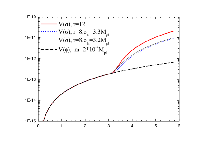
Figure 1: Effective potentials $V(\sigma)$ together with $V(\phi_{1})$. The horizontal axis is the value of inflaton $\phi_{1}$ or $\sigma$, in unit of $M_{pl}$. The vertical axis delineates the inflaton potential, in unit of $M^{4}_{pl}$.

We notice, from Fig. 1, $\dot{\sigma}$ achieves a large value during the transition time and the scalar power perturbation is suppressed via the slow-rolling(SR) formula $P_{S}\propto(\frac{H^{2}}{2\pi\dot{\sigma}})^{2}$. The SR parameters $\epsilon$ and $\delta$ during the transition are

$$\epsilon\equiv-\frac{\dot{H}}{H^{2}}=4\pi G(\frac{\dot{\sigma}}{H})^{2}\approx\frac{3}{2}\frac{\dot{\phi_{2}}^{2}}{\rho_{\phi_{1}}+\rho_{\phi_{2}}}~{},$$ (8)

and

$$\delta\equiv\frac{\ddot{\sigma}}{H\dot{\sigma}}=\frac{\dot{\phi_{1}}\ddot{\phi_{1}}+\dot{\phi_{2}}\ddot{\phi_{2}}}{H(\dot{\phi_{1}}^{2}+\dot{\phi_{2}}^{2})}\approx-\frac{3\dot{\phi_{2}}^{2}}{\dot{\phi_{1}}^{2}+\dot{\phi_{2}}^{2}}~{}.$$ (9)

We notice that when $\phi_{2}$ oscillates, $\rho_{\phi_{2}}\sim\dot{\phi_{2}}^{2}\propto a^{-3}$, $\epsilon$ and $-\delta$ reach their local maximum values. One can also find the maximum value $(-\delta)_{max}>\epsilon_{max}$. In the extreme limit when $V(\phi_{1})$ is negligible during the transition one has $(-\delta)_{max}=3$ and $\epsilon_{max}=1.5$. Regarding the fore-mentioned four parameters, the ratio $r\equiv M_{2}/M_{1}$ and the initial value of $\phi_{1}$, determine the locations and values of $-\delta_{max}$ and $\epsilon_{max}$. The maximal values are mainly determined by $r$. If the ratio $r$ is too small (e.g. $1\leq r\lesssim 3$) the above picture cannot be realized because both fields would take effect during inflation and neither is negligible. While $r$ is too large (e.g. $r\gtrsim 11$) one gets $1+\epsilon+\delta<0$ during the transition and superhorizon effectsLeach:2000yw would take place. The perturbations do get suppressed at some smaller $k$ but enhanced around certain larger $k$ values. Under such circumstances the whole effect might be negative to achieve small CMB TT quadrupole. The need that $P_{S}(k)$ be suppressed at small $k$ requires some tuning of the initial value of $\phi_{1}$. $M_{1}$ determines the amplitude of the perturbation and is normalized by the current observations. The initial value of $\phi_{2}$ is arbitrary with a weak prior to provide enough number of $e-folding$ to solve the flatness problem.

As our model parameters lie in the region where SR approximation does not work well, we calculate the primordial scalar and tensor spectra using mode by mode integrationswenbin ; wangxl ; fengbo2 . We denote the scale where $P_{S}$ arrives around its local maximum as $k_{f}$ and tune the initial $\phi_{1}$ to get $N(k_{f})\sim 55$.

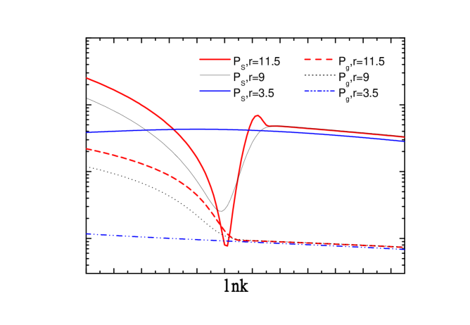
Figure 2: Primordial scalar $P_{s}$ and tensor spectra $P_{g}$ for $r=3.5$, 9 and 11.5. The overall amplitude can be normalized by WMAP.

In Fig. 2 we show the numerical results of the scalar and tensor spectra for $r=3.5$, 9 and 11.5. One can see that, for $r=3.5$, the spectra is almost featureless while well suppressed scalar spectra have been generated for $r=9$ and 11.5. For the example of $r=11.5$ $P_{S}$ is enhanced around $k_{f}$ due to the superhorizon contributionsLeach:2000yw .

We then fit the resulting primordial spectra to the current WMAP TT and TE data. As shown in Refs.Lyth reports ; fgw , in such inflation models one cannot know the exact values of $k_{f}$ due to the uncertainty in the details of reheating. So $\ln k_{f}$ is another parameter in our model. Our fitting is similar to Ref.fengbo2 : We fix $\Omega_{b}h^{2}=0.022$, $\Omega_{m}h^{2}=0.135$, $\tau_{c}=0.17$, $\Omega_{\rm tot}=1$ Spergel and set $\Omega_{\Lambda}$ and $\ln k_{f}$ as free parameters in our fit. Denoting $k_{c}=7.0\times 70./3/10^{5}\approx 1.6\times 10^{-3}$ Mpc^-1, we vary grid points with ranges $[0.68,0.77]$, and $[-3,5.]$ for $\Omega_{\Lambda}$ and $\ln(k_{f}/k_{c})$, respectively. $M_{2}/M_{1}$ varies from 3.5 to 12 in step of 0.5. At each point in the grid we use subroutines derived from those made available by the WMAP team to evaluate the likelihood with respect to the WMAP TT and TE data Verde . The overall amplitude of the primordial perturbations has been used as a continuous parameter.

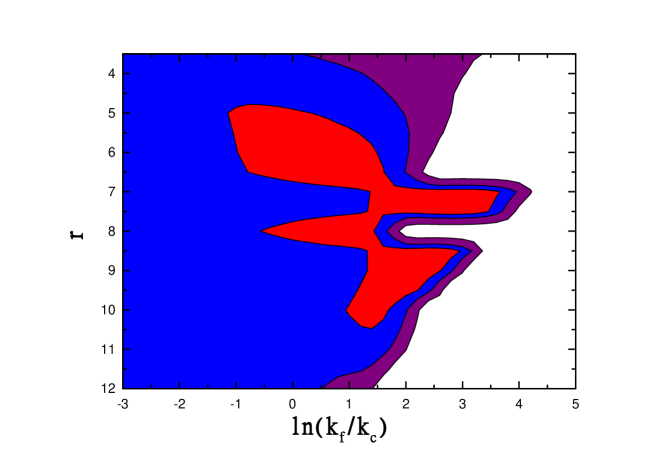
Figure 3: Two-dimensional contours in the r– $\ln(k_{f}/k_{c})$ plane for our grids of model. $k_{c}\approx 1.6\times 10^{-3}$ Mpc^-1. The regions of different color show $1.1\sigma$, 2 and $3\sigma$ confidence respectively.

In Fig. 3 we plot the resulting $\chi^{2}$ values as functions of $r$ and $\ln(k_{f}/k_{c})$. The contours shown are for $\Delta\chi^{2}$ values giving 1.1, 2, and 3 $\sigma$ contours for two parameter Gaussian distributions. As the location is rather hard to be fixed at exactly $N(k_{f})=55$, the figure is not very smooth as expected.

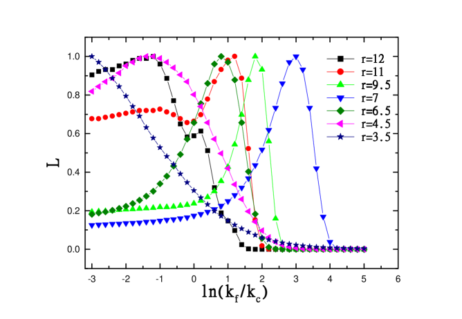
Figure 4: One-dimensional marginalized distributions of $\ln(k_{f}/k_{c})$ for $r=3.5$, 4.5, 6.5, 7, 9.5, 11 and 12.

Our main intention is to see how the primordial spectrum with a feature is favored by WMAP. This can be also seen in the one-dimensional marginalized distribution of $\ln(k_{f}/k_{c})$ for each $r$. To see clearly how the feature is favored, we do not marginalize over $r$ and show some of them in Fig. 4. For $r=3.5$, $k_{f}\sim 0$ is favored and when $r=7$, $\ln(k_{f}/k_{c})=3$ is favored at around $2\sigma$. $k_{f}\sim 0$ is excluded at less than $1\sigma$ for $r=4.5$ where $P_{S}$ is not suppressed enough around $k_{f}$. While for $r\gtrsim 11$, $P_{S}$ is enhanced around $k_{f}$ and although nonzero $k_{f}$ is favored for shown examples, $k_{f}\sim 0$ is excluded at less than $1\sigma$. We find that, for $6\lesssim r\lesssim 10$, nonzero $k_{f}$ is favored at $\gtrsim 1.5\sigma$. For the investigated parameter space with $3.5\lesssim r\lesssim 12$ we have $P_{S}(0.05/Mpc)=2.46\sim 2.59\times 10^{-9}$ at $2\sigma$ level. This gives $M_{1}\sim 1.7\times 10^{13}$ GeV.

A detailed analysis gives the e-folds number $N(k)$ before the end of inflationLyth reports ; fgw :

$$N(k)=60.56-\ln h-\ln\frac{k}{a_{0}H_{0}}-\ln\frac{10^{16}GeV}{\rho(k)^{1/4}}+\ln\frac{\rho(k)^{1/4}}{\rho_{end}^{1/4}}-\frac{1}{3}\ln\frac{\rho_{end}^{1/4}}{\rho_{RH}^{1/4}}\ \ ,$$ (10)

where $\rho(k)$, $\rho_{end}$ denote the inflaton potential at $k=aH$ and at the end of inflation respectively, $\rho_{RH}$ is the energy density when reheating ends, resuming a standard big bang evolution. Since in our case there is a preferred scale $\ln(k_{f}/k_{c})$ while $N(k_{f})$ is fixed around 55, the reheating energy may be determined by the current observations. However, one can see that the location of $k_{f}$ is mainly determined by the initial value of $\phi_{1}$. Once the initial $\phi_{1}$ changes, $N(k_{f})$ will change and the resulting $\rho_{RH}$ would be different. We show the case in Fig. 5 as an example. For $r=8$, $\phi_{1i}=3.2$ and $3.3M_{pl}$ lead to $N(k_{f})=54.34$ and 59.06 respectively. We get $P_{S}\sim 2.5\times 10^{-9}$ at 0.05 Mpc^-1, the resulting $\ln(k_{f}/k_{c})=(-1.7,1.3)$ and $(0.1,1.9)$ at $2\sigma$ respectively. We also have $h\approx 0.73$, $\rho^{\frac{1}{4}}(0.05/Mpc)\sim 1.8\times 10^{-3}M_{pl}$ and $\rho^{\frac{1}{4}}_{end}\sim 5.1\times 10^{-4}M_{pl}$. Taking these to the models we get $\rho^{\frac{1}{4}}_{RH}=(8.5\times 10^{4}GeV,6.9\times 10^{8}GeV)$ and $(2.6\times 10^{13}GeV,5.8\times 10^{15}GeV)$ at $2\sigma$ for the two different $\phi_{1i}$. Therefore, the reheating temperature is fully correlated with initial $\phi_{1}$ in this model.

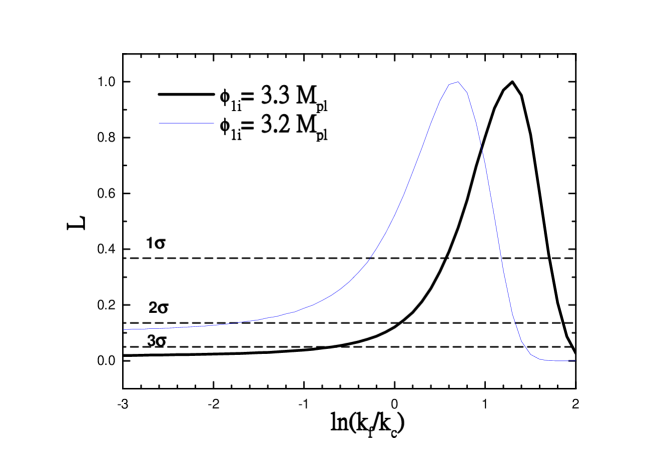
Figure 5: One dimensional likelihoods of r=8, $\phi_{1i}=3.2$ and 3.3 $M_{pl}$.

We get our minimum $\chi^{2}=1429.1$ when $r=8.5$ and $\ln(k_{f}/k_{c})=2.4$. When compared with the standard power-law $\Lambda$CDM model, we have minimum $\chi^{2}=1432.7$ and $\Delta\chi^{2}=-3.6$. For the single field chaotic inflation we get minimum $\chi^{2}=1432.9$, with $\Delta\chi^{2}=-3.8$. However, in the sneutrino inflation, we have to set $\rho_{RH}^{\frac{1}{4}}\lesssim 10^{10}$ GeV due to the gravitino problemgravitino . In this case, we get $N(k_{c})\lesssim 55.5$ and minimum $\chi^{2}=1433.2$, which gives $\Delta\chi^{2}=-4.1$. In addition, there are only two parameters, the mass and $\ln(k_{f}/k_{c})$, in the single field sneutrino inflation model. This indicates our double sneutrino inflation is favored at $\sim 1.5\sigma$ by WMAP than the single field sneutrino inflation. In Fig. 6 we show the resulting CMB TT multipoles and two-point temperature correlation function for single and double field sneutrino inflation in our parameter space. One can see that the resulting CMB TT quadrupole and the correlation function at $\theta\gtrsim 60^{\circ}$ are much better suppressed in the double sneutrino inflation than in the single sneutrino model. In fact, the spectrum of the single field sneutrino inflation is equivalent to that in our double case with $r=1$ and $\phi_{1i}=\phi_{2i}$. In this sense we get $6\lesssim r\lesssim 10$ is favored at $\gtrsim 1.5\sigma$ ($\Delta\chi^{2}\lesssim-2.3$) than $r=1$ in double sneutrino inflation.

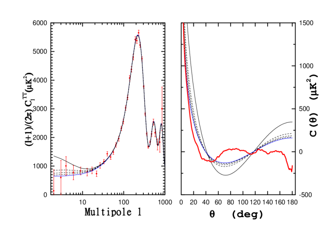
Figure 6: CMB anisotropy and two-point temperature correlation function for single and double field sneutrino inflation. Left: From left top to bottom, the lines stand for single sneutrino inflation, double sneutrino inflation with $\ln(k_{f}/k_{c})=3.0$, 3.2, 3.4 and 3.6. $r$ is fixed at 8.5. Right: From right top to bottom, the lines stand for single sneutrino inflation, double sneutrino inflation with $\ln(k_{f}/k_{c})=3.0$, 3.2, 3.4 and 3.6 and the WMAP released data.

Finally, it is worth mentioning that we have also considered a double inflaton model with quartic potential

$$V(\phi_{1},\phi_{2})=\lambda_{1}\phi_{1}^{4}+\lambda_{2}\phi_{2}^{4}~{}.$$ (11)

As we known, the quartic potential $\lambda\phi^{4}$ is disfavored by the current WMAP and LSS observations, because it has a larger tensor perturbation. Peiris et al. Peiris fix the number of e-folding at 50 and find $\lambda\phi^{4}$ inflation model is excluded at more than $3\sigma$ by WMAP and 2DFGRS data. WMAP alone excludes $\lambda\phi^{4}$ inflation at more than $99\%$ confidence level when $N\sim 50$. The discrepancy between the theoretical predictions and observations comes mainly from the contributions of small CMB multipoles. In the double inflaton quartic model, the CMB quadruples can also be well suppressed and the model is also favored by WMAP. We fix $N(k_{f})=50$ and run two codes, one with $\lambda_{2}/\lambda_{1}=6400$ and the other with $\lambda_{2}/\lambda_{1}=3600$ and fit the primordial scalar and tensor spectra to WMAP TT and TE data. We get minimum $\chi^{2}=1427.9$ and $1428$ respectively. They work better than the double quadratic sneutrino inflation. Reheating temperature in this case cannot be restricted from WMAP, as shown in Ref.liddle .

III phenomenology

In the minimal seesaw mechanism, the right-handed sector is least known. However, in the double sneutrino inflation model, two neutrino masses $M_{1}$ and $M_{2}$ are constrained by the WMAP as shown in the previous section. In the following, we will study the phenomenological implications of this model, including the reheating temperature, leptogenesis, lepton flavor violation and neutrinoless double beta decay.

III.1 Parameterization of the minimal seesaw model

In this subsection we present our convention and parameterization of the minimal supersymmetric seesaw model. At the energy scales above the RH neutrino masses, the superpotential of the lepton sector is given by

$$W=Y_{L}^{ij*}\hat{H}_{1}\hat{L}_{i}\hat{E}_{j}+Y_{N}^{ij*}\hat{H}_{2}\hat{L}_{i}\hat{N}_{j}+\frac{1}{2}M_{R}^{ij*}\hat{N}_{i}\hat{N}_{j}+\mu\hat{H}_{1}\hat{H}_{2}\ \ ,$$ (12)

where $Y_{L}$ and $Y_{N}$ are the charged lepton and neutrino Yukawa coupling matrices, respectively, $M_{R}$ is the Majorana mass matrix for the right-handed neutrinos, with $i$ and $j$ being the generation indices.

Generally, $Y_{L}$ and $Y_{N}$ can not be diagonalized simultaneously. This mismatch leads to the lepton flavor violating (LFV) interactions. The three matrices $Y_{L}$, $Y_{N}$ and $M_{R}$ can be diagonalized by

$$Y^{\delta}_{L} = U_{L}^{\dagger}Y_{L}U_{R}\ \ ,$$ (13)

$$Y^{\delta}_{N} = V_{L}^{\dagger}Y_{N}V_{R}\ \ ,$$ (14)

$$M_{R}^{\delta} = XV_{R}^{T}M_{R}V_{R}X^{T}\ \ ,$$ (15)

respectively, where $U_{L,R}$ , $V_{L,R}$ and $X$ are all unitary matrices.

We can define the lepton flavor mixing matrix $V$, the analog to the Kobayashi-Maskawa matrix $V_{KM}$ in the quark sector, as

$$V=U_{L}^{\dagger}V_{L}\ .$$ (16)

$V$ is determined by the left-handed mixing of the Yukawa coupling matrices $Y_{L}$ and $Y_{N}$, and only exists above the energy scales $M_{R}$. We will see below that this matrix determines the LFV effects in the supersymmetric seesaw model at low energies.

We then rotate the bases of $\hat{L}$, $\hat{E}$ and $\hat{N}$ to make both $Y_{L}$ and $M_{R}$ diagonal. On this basis, $Y_{N}$ can be written in a general form as

$$Y_{N}=VY^{\delta}X^{T}\ .$$ (17)

By adjusting the phases of the superfields, $V$ is a CKM-like mixing matrix with one physical CP phase, and $X$ has the form

$$X=\left(\begin{array}[]{ccc}1&&\\ &e^{i\alpha}&\\ &&e^{i\beta}\end{array}\right)\tilde{X}\left(\begin{array}[]{ccc}1&&\\ &e^{i\rho}&\\ &&e^{i\omega}\end{array}\right)\ ,$$ (18)

where $\alpha$, $\beta$, $\rho$ and $\omega$ are Majorana phases and $\tilde{X}$ is a CKM-like mixing matrix with another Dirac CP phase. It is then easy to count that there are 18 parameters to parametrize the minimal seesaw mechanism, which include 6 Yukawa coupling constants (or mass) eigenvalues in $Y_{N}$ and $M_{R}$, 6 mixing angles and 6 CP phases in $V$ and $X$.

At low energies, the heavy RH neutrinos are integrated out and the Majorana mass matrix for the left-handed neutrinos is given by

$$m_{\nu}=-m_{N}\frac{1}{M_{R}}m_{N}^{T}\ ,$$ (19)

where $m_{N}=Y_{N}v\sin\beta$ is the neutrino Dirac mass matrix, with $v$ being the vacuum expectation value (VEV) of the Higgs boson. $m_{\nu}$ can be diagonalized by

$$U_{\nu}^{\dagger}m_{\nu}U_{\nu}^{*}=m_{\nu}^{\delta}\ ,$$ (20)

where $U_{\nu}=\tilde{U}_{\nu}\cdot\text{diag}(1,e^{i\eta},e^{i\xi})$ is the MNS mixing matrixMNS , with $\eta$, $\xi$ being low energy Majorana CP phases. $U_{\nu}$ describes the neutrino mixing at low energies, which is different from the high energy mixing matrix $V$ defined in Eq. (16). From Eq. (19) we can see that $m_{\nu}$ is related to all the 18 seesaw parameters. However, measuring $m_{\nu}$ at low energy only determines 9 of the 18 seesaw parameters. We will see below that leptogenesis and lepton flavor violation are related to different combinations of the 18 seesaw parameters and can provide different information to determine the seesaw parameters from the $\nu$-oscillation and LFV observations.

We can rewrite the seesaw formula Eq. (19) in another form

$$U_{\nu}\sqrt{m_{\nu}^{\delta}}\left(U_{\nu}\sqrt{m_{\nu}^{\delta}}\right)^{T}=-Vm_{N}^{\delta}X^{T}\frac{1}{\sqrt{M_{R}^{\delta}}}\left(Vm_{N}^{\delta}X^{T}\frac{1}{\sqrt{M_{R}^{\delta}}}\right)^{T}\ ,$$ (21)

from which $m_{N}$ can be solved in terms of the left- and right-handed neutrino masses,

$$m_{N}^{\delta}=V^{\prime\dagger}\sqrt{m_{\nu}^{\delta}}\hat{O}^{T}\sqrt{M_{R}^{\delta}}\tilde{X}^{*}\ ,$$ (22)

where $\hat{O}$ is an arbitrary orthogonal $3\times 3$ matrixcasas and $V^{\prime}=\tilde{U}_{\nu}^{\dagger}V$. In the above equation we have absorbed all the 6 Majorana CP phases in the diagonal eigenvalue matrices: two low energy Majorana phases, $\eta$, $\xi$, are absorbed by $\sqrt{m_{\nu}^{\delta}}$ and the four high energy Majorana phases, $\alpha$, $\beta$, $\rho$, $\omega$, are absorbed by $m_{N}^{\delta}$ and $\sqrt{M_{R}^{\delta}}$. We will use this equation repeatedly in the following discussions.

III.2 The reheating temperature

The lightest sneutrino $\tilde{N}_{1}$ begins to oscillate when the Hubble expansion rate $H\sim M_{1}$ and decays at $H\sim\Gamma_{\tilde{N}_{1}}$. The Universe is then reheated by the relativistic decay products. The reheating temperature is approximately determined by

$$T_{RH}\approx\left(\frac{90}{\pi^{2}g_{*}}\right)^{\frac{1}{4}}\sqrt{\Gamma_{\tilde{N}_{1}}M_{P}}\ ,$$ (23)

where $g_{*}$ is the number of the effective relativistic degrees of freedom in the reheated Universe, $M_{P}=1/\sqrt{8\pi G_{N}}\simeq 2.4\times 10^{18}GeV$ is the Planck scale, and

$$\Gamma_{\tilde{N}_{1}}=\frac{1}{4\pi}(Y_{N}^{\dagger}Y_{N})_{11}M_{1}\ ,$$ (24)

is the width of the lightest sneutrino $\tilde{N}_{1}$, if it couples to other matter only through the Yukawa coupling in Eq. (12). Taking $M_{1}\approx 1.7\times 10^{13}GeV$ and $T_{RH}\sim 10^{10}GeV$, we get $(Y_{N}^{\dagger}Y_{N})_{11}$ should be as small as $\mathcal{O}(10^{-10})$.

The reheating temperature (as well as leptogenesis) is related to the RH mixing of $Y_{N}$ and put strong constraints on this mixing matrix. Using Eq. (17), we have

$$(Y_{N}^{\dagger}Y_{N})_{11}=(X^{*}({Y^{\delta}})^{2}X^{T})_{11}=(\tilde{X}^{*}({Y^{\delta}})^{2}\tilde{X}^{T})_{11}=|\tilde{X}_{1i}|^{2}Y_{i}^{2}\ .$$ (25)

The elements $|\tilde{X}_{1i}|$ can be parametrized by two mixing angles, $\theta_{1,2}$. We then get

$$(Y_{N}^{\dagger}Y_{N})_{11}=c_{1}^{2}c_{2}^{2}Y_{1}^{2}+c_{1}^{2}s_{2}^{2}Y_{2}^{2}+s_{1}^{2}Y_{3}^{2}\approx Y_{1}^{2}+s_{2}^{2}Y_{2}^{2}+s_{1}^{2}Y_{3}^{2}\approx 10^{-10}\ ,$$ (26)

with $c_{i}=\cos{\theta_{i}}$, $s_{i}=\sin{\theta_{i}}$. In the later discussion we will see that $Y_{2}$ is $\mathcal{O}(0.1)$ and $Y_{3}$ is $\mathcal{O}(1)$. Then we have

$$Y_{1}^{2}\lesssim 10^{-10}\ ,\ s_{2}^{2}\lesssim 10^{-8}\ ,\ s_{1}^{2}\lesssim 10^{-10}\ .$$ (27)

Since $\theta_{1,2}$ are extremely small, $\tilde{X}$ can be given in a quite simple form as

$$\tilde{X}\approx\left(\begin{array}[]{ccc}1&s_{2}&\hat{s}_{1}\\ -(c_{3}s_{2}+s_{3}\hat{s}_{1}^{*})&c_{3}&s_{3}\\ s_{3}s_{2}-c_{3}\hat{s}_{1}^{*}&-s_{3}&c_{3}\end{array}\right)\ ,$$ (28)

where $\hat{s}_{1}=s_{1}e^{i\delta}$.

Using Eqs. (22) and (24), we have

$$(m_{N}^{\dagger}m_{N})_{11} = \frac{4\pi\Gamma_{\tilde{N}_{1}}}{M_{1}}(v\sin\beta)^{2}\approx 4\times 10^{-6}\left(\frac{T_{RH}}{10^{10}GeV}\right)^{2}GeV^{2}$$ (29)

$$\approx M_{1}m_{\nu_{1}}|\hat{O}_{11}|^{2}+120.7GeV^{2}|\hat{O}_{12}|^{2}+850GeV^{2}|\hat{O}_{13}|^{2}\ ,$$

where we have assumed $\sin\beta\approx 1$ for large $\tan\beta$, and $m_{\nu_{2}}\approx\sqrt{\Delta m_{sol}^{2}}\approx 7.1\times 10^{-3}eV$ and $m_{\nu_{3}}\approx\sqrt{\Delta m_{atm}^{2}}\approx 0.05eV$. From the above equation we can see that $\hat{O}_{12}$ and $\hat{O}_{13}$ have to be negligibly small. We will set these two elements zero and write $\hat{O}$ as

$$\hat{O}=\left(\begin{array}[]{ccc}\pm 1&&\\ &\hat{c}&\hat{s}\\ &-\hat{s}&\hat{c}\end{array}\right)\ ,$$ (30)

where $\hat{c}=\cos\theta_{T}$, $\hat{s}=\sin\theta_{T}$ with $\theta_{T}$ being an arbitrary complex angle. (It should be noted that $\hat{O}_{12}$ and $\hat{O}_{13}$ can not be exactly zero, since if they are zero the first-generation right-handed (s)neutrino decouples from the other two generations and no lepton number asymmetry can be induced when it decays. However, the tiny mixing has no effect on lepton flavor violation and we can ignore them safely when discussing LFV.)

From Eq. (29) we can estimate that

$$m_{\nu_{1}}\approx\left\{\begin{array}[]{l}2.\times 10^{-10}eV,\ \ \text{for}\ \ T_{RH}=10^{10}GeV\ ,\\ 2.\times 10^{-12}eV,\ \ \text{for}\ \ T_{RH}=10^{9}GeV\ .\end{array}\right.$$ (31)

This estimation is correct when the last two terms are much smaller than the first one in the second line of Eq. (29), or, equivalently, the $Y_{1}$ term dominants the others in Eq. (26). In the following discussion for leptogenesis we will see that this is a quite natural situation.

III.3 Leptogenesis

Since the reheating temperature, $T_{RH}$, is far below the lightest RH (s)neutrino mass, $M_{1}$, leptogenesis arises dominantly from direct cold sneutrino decays, with negligible thermal wash-out effects. In this case, the baryon asymmetry is given byhamaguchi

$$Y_{B}\equiv\frac{n_{B}}{s}=a\frac{3}{4}\epsilon_{1}\frac{T_{RH}}{M_{1}}\ ,$$ (32)

where $a=-8/23$ is the ratio of baryon to lepton asymmetry balanced by the “sphaleron” process. In order to produce the observed baryon asymmetry in the Universe, $Y_{B}\sim 10^{-10}$, we require the sneutrino decay asymmetry $\epsilon_{1}\sim-10^{-6}$. The asymmetry $\epsilon_{1}$ is given by

$$\epsilon_{1}\approx-\frac{3}{16\pi}\frac{1}{(Y_{N}^{\dagger}Y_{N})_{11}}\sum_{i=2,3}\text{Im}\left[(Y_{N}^{\dagger}Y_{N})_{1i}\right]^{2}\frac{M_{1}}{M_{i}}\ .$$ (33)

Using the expression for $\tilde{X}$ in Eq. (28) and the large hierarchy between $Y_{1}$ and $Y_{2}$, $Y_{3}$ we get

$$(Y_{N}^{\dagger}Y_{N})_{12} \approx (s_{2}Y_{2}^{2}+\hat{s}_{1}^{*}s_{3}Y_{3}^{2})e^{i\alpha}\ ,$$

$$(Y_{N}^{\dagger}Y_{N})_{13} \approx (-s_{2}s_{3}Y_{2}^{2}+\hat{s}_{1}^{*}Y_{3}^{2})e^{i\beta}\ .$$ (34)

We will discuss two simple cases to illustrate some quantitative features of the seesaw parameters required by leptogenesis. We will see that, in Eq. (26), the $Y_{2}$ and $Y_{3}$ terms should be smaller than the $Y_{1}$ term in order to produce the lepton number asymmetry at the correct order.

• Case I, $s_{1}Y_{3}^{2}\ll s_{2}Y_{2}^{2}$

  In this case the expression for $\epsilon_{1}$ is simplified as

  $$\epsilon_{1} \approx -\frac{3}{16\pi}\frac{1}{(Y_{N}^{\dagger}Y_{N})_{11}}\left[({s_{2}Y_{2}^{2}})^{2}\sin 2\alpha\frac{M_{1}}{M_{2}}+(s_{2}s_{3}Y_{2}^{2})^{2}\sin 2\beta\frac{M_{1}}{M_{3}}\right]$$ (35)

  $$\sim -10^{-4}\cdot\frac{s_{2}^{2}Y_{2}^{2}}{Y_{1}^{2}+s_{2}^{2}Y_{2}^{2}}\cdot\sin 2\alpha\ .$$

  When deriving the second line we have assumed that $\alpha$ and $\beta$ are of the same order and $\frac{M_{1}}{M_{3}}\ll\frac{M_{1}}{M_{2}}\sim Y_{2}\sim 0.1$ and $s^{2}_{1}Y_{3}^{2}\ll s^{2}_{2}Y_{2}^{2}$. If the CP phases are of order 1, $s_{2}^{2}Y_{2}^{2}/Y_{1}^{2}$ should be at the order of about $10^{-2}$. Actually, this case corresponds to the maximal asymmetry given by $|\epsilon_{1}^{max}|\approx\frac{3}{16\pi}\frac{M_{1}\sqrt{\Delta m_{sol}^{2}}}{v^{2}}\sim 10^{-4}$ buch . In this case, the CP phase or, $s_{2}^{2}Y_{2}^{2}/(Y_{N}^{\dagger}Y_{N})_{11}$, has to be at the order of $\mathcal{O}(10^{-2})$.

• Case II, $s_{1}\sim s_{2}$

  In this case we can simplify the expression for $\epsilon_{1}$ as

  $$\epsilon_{1} \approx -\frac{3}{16\pi}\frac{1}{(Y_{N}^{\dagger}Y_{N})_{11}}\left[({s_{1}s_{3}Y_{3}^{2}})^{2}\sin 2\alpha^{\prime}\frac{M_{1}}{M_{2}}+(s_{1}Y_{3}^{2})^{2}\sin 2\beta^{\prime}\frac{M_{1}}{M_{3}}\right]$$ (36)

  $$\sim -10^{-3}\cdot\frac{s_{1}^{2}Y_{3}^{2}}{Y_{1}^{2}+s_{1}^{2}Y_{3}^{2}}\cdot(\sin 2\alpha^{\prime}+\sin 2\beta^{\prime})\ ,$$

  where we have used the fact that $s_{3}\sim\sqrt{M_{2}/M_{3}}$ if $\theta_{T}$ is of order $1$, $s^{2}_{1}Y_{3}^{2}\gg s^{2}_{2}Y_{2}^{2}$ and $\alpha^{\prime}=\alpha-\delta$, $\beta^{\prime}=\beta-\delta$. Similar to Case I, we get that $s_{1}^{2}Y_{3}^{2}/Y_{1}^{2}$ should be at the order of $10^{-3}$ if the CP phases are of order 1. In this case, the maximal asymmetry is $|\epsilon_{1}^{max}|\approx\frac{3}{16\pi}\frac{M_{1}\sqrt{\Delta m_{atm}^{2}}}{v^{2}}\sim 10^{-3}$.

Certainly, it is possible that the contributions to $(Y_{N}^{\dagger}Y_{N})_{11}$ from $Y_{2}$ and $Y_{3}$ in Eq. (26) are of the same order. In this case we also expect that these values be correct as an estimate of the order of magnitude, i.e., $s^{2}_{1}Y_{3}^{2}\sim s^{2}_{2}Y_{2}^{2}\ll Y^{2}_{1}$. This analysis justifies our guess in the last subsection that the $Y_{1}$ term gives the dominant contribution in the process of reheating the Universe. Conversely, if the $Y_{2}$ or $Y_{3}$ term gives dominant contribution, the CP phases have to be fine tuned to the order of $10^{-2}$ and $10^{-3}$ respectively, in order not to create too much lepton number asymmetry and $m_{\nu_{1}}$ in Eq. (31) will be even smaller.

III.4 Lepton flavor violation and muon anomalous magnetic moment

We have shown that leptogenesis is associated with the high energy mixing angles and CP phases in the unitary matrix $X$. Generally, leptogenesis has no direct relation with the low energy neutrino phenomena. However, another interesting phenomena — the charged lepton flavor violating decays — predicted by this sneutrino inflaton model, can provide constraints on the seesaw model’s parameter space. The muon anomalous magnetic moment is also considered to constrain the SUSY parameters.

In a supersymmetric model, the present experimental limits on the LFV processes has put very strong constraints on the soft supersymmetry breaking parameters, with the strongest constraints coming from the process $\mu\to e\gamma$ (BR$(\mu\to e\gamma)<1.2\times 10^{-11}$mueg ). It is a usual practice to assume universal soft SUSY breaking parameters $m_{0}$, $m_{1/2}$ and $A_{0}$ at the SUSY breaking scale ( We take it the GUT scale here) to suppress the LFV effects. However, since there are LFV interactions in the seesaw models, the lepton flavor violating off-diagonal elements of $(m_{\tilde{L}}^{2})_{ij}$, the slepton doublet soft mass matrix, and $({A_{e}})_{ij}$, the lepton soft trilinear couplings, can be induced when running the renormalization group equations (RGEs) for $m_{\tilde{L}}^{2}$ and ${A_{e}}$ between $M_{GUT}$ and $M_{R}$.

The off-diagonal elements of $(m_{\tilde{L}}^{2})_{ij}$ and $({A_{e}})_{ij}$ can be approximately given by

$$\left(\delta m_{\tilde{L}}^{2}\right)_{ij} \approx \frac{1}{8\pi^{2}}(Y_{N}Y_{N}^{\dagger})_{ij}(3+a^{2})m_{0}^{2}\log\frac{M_{GUT}}{{M_{R}}}\ ,$$ (37)

$$\left(\delta A_{e}\right)_{ij} \approx \frac{1}{8\pi^{2}}(Y_{N}Y_{N}^{\dagger})_{ij}am_{0}\log\frac{M_{GUT}}{{M_{R}}}\ ,$$ (38)

where $A_{0}=am_{0}$ is the universal trilinear coupling at $M_{GUT}$. Using Eq. (17) we have

$$(Y_{N}Y_{N}^{\dagger})_{ij} = (V(Y_{N}^{\delta})^{2}V^{\dagger})_{ij}\approx V_{i2}V_{j2}^{*}Y_{2}^{2}+V_{i3}V_{j3}^{*}Y_{3}^{2}\ ,\ \ \text{for}\ M_{GUT}>Q>M_{3}$$

$$= \sum_{k=1,2}(VY_{N}^{\delta}X^{T})_{ik}(X^{*}Y_{N}^{\delta}V^{\dagger})_{kj}$$

$$\approx \sum_{l,m=2,3}V_{il}V_{jm}^{*}Y_{l}Y_{m}(\delta_{lm}-X_{3l}X_{3m}^{*})\ ,\ \ \text{for}\ M_{3}>Q>M_{2}\ .$$ (40)

The numerical result shows that, since the mixing angles in $X$ are all small, the LFV effects are only sensitive to the left-handed mixing matrix $V$, while leptogenesis only relies on the right-handed mixing matrix $X$. Thus, there are no direct relation between the two phenomena in principle.

We have solved the full coupled RGEs numerically from the GUT scale to $M_{Z}$ scale. At the energy scales below $M_{2}$ we solve the RGEs for MSSM and below $M_{SUSY}$ the RGEs return to those of the SM.

In principle, only 9 of the 18 seesaw parameters are determined in our model, i.e., $m_{\nu_{i}}$, $M_{i}$ and 3 low energy neutrino mixing angles. In order to predict the branching ratio of the LFV decays, we have to explore a 9-dimensional parameter space of the unknown variables. However, from our previous discussions, we know that the relevant seesaw parameters to LFV are reduced to only 4 in this model, which can be chosen as 1 complex angle $\theta_{T}$, and 2 CP phases. We can explicitly write the ‘reduced’ seesaw formula for the 2nd and 3rd generations as

$$\left(\begin{array}[]{cc}m_{N_{2}}&\\ &m_{N_{3}}e^{i\omega^{\prime}}\end{array}\right) = V^{\prime\dagger}\left(\begin{array}[]{cc}\sqrt{m_{\nu_{2}}}&\\ &\sqrt{m_{\nu_{3}}}e^{i\phi_{1}}\end{array}\right)\left(\begin{array}[]{cc}\hat{c}&-\hat{s}\\ \hat{s}&\hat{c}\end{array}\right)\left(\begin{array}[]{cc}\sqrt{M_{2}}&\\ &\sqrt{M_{3}}e^{i\phi_{2}}\end{array}\right)\tilde{X}$$ (49)

$$= V^{\prime\dagger}\left(\begin{array}[]{cc}1&\\ &e^{i\phi_{1}}\end{array}\right)\mathcal{M}\left(\begin{array}[]{cc}1&\\ &e^{i\phi_{2}}\end{array}\right)\tilde{X}\ ,$$ (54)

where both $V^{\prime}$ and $\tilde{X}$ are $2\times 2$ real orthogonal matrices, determined by diagonalizing the matrix $\mathcal{M}$. Here, we adopt the running values of $m_{\nu_{2}}$ and $m_{\nu_{3}}$ at the scale of $10^{14}GeV$ratz . Once $Y_{2,3}$ and $V=U_{\nu}V^{\prime}$ are determined, can we calculate the LFV branching ratios, BR($l_{i}\to l_{j}\gamma$).

The relevant parameters to investigate BR($l_{i}\to l_{j}\gamma$) and $\delta a_{\mu}$ include the mSUGRA parameters: $m_{0}$, $m_{1/2}$, $A_{0}$, $\tan\beta$, $\text{sgn}(\mu)$ and the seesaw parameters: $\theta_{T}$ and $\phi_{i}$. Since BR($l_{i}\to l_{j}\gamma$) and $\delta a_{\mu}$ nearly scale with $\tan^{2}\beta$ and $\tan\beta$ respectively, we take $\tan\beta=10$ as a representative value. We fix $A_{0}=0$ through our calculation since it has small influence on the numerical results. The Higgsino mass parameter $\mu>0$ is assumed, motivated by the $g_{\mu}-2$ anomaly. As for the seesaw parameters, we take $\Delta m_{sol}^{2}=5\times 10^{-5}eV^{2}$, $\Delta m_{atm}^{2}=2.5\times 10^{-3}eV^{2}$, and $\tan^{2}\theta_{12}=0.42$, $\sin^{2}2\theta_{23}=1$, $0<\theta_{13}<0.2$ from the neutrino oscillation experiments. We fix $M_{1}=1.7\times 10^{13}GeV$, $M_{2}=10^{14}GeV$ and $4\times 10^{14}GeV<M_{3}<1\times 10^{16}GeV$ for RH heavy Majorana neutrinos.

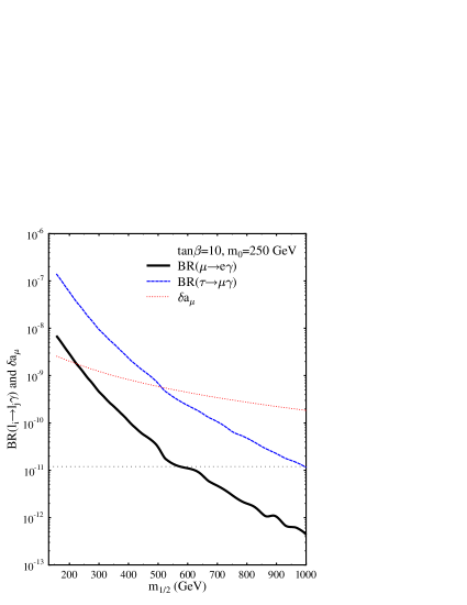
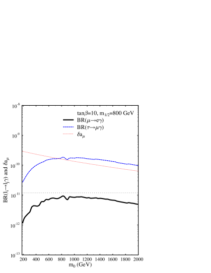
Figure 7: BR($l_{i}\to l_{j}\gamma$) and $\delta a_{\mu}$ as a function of $m_{1/2}$ and $m_{0}$ in the left and right panels respectively. $\tan\beta=10$, $A_{0}=0$ and $\mu>0$ are fixed. We take $m_{0}=250GeV$ for the left panel and $m_{1/2}=800GeV$ for the right panel. The seesaw parameters are taken as $\theta_{T}=\pi/4$, $\phi_{i}=0$, $\theta_{13}=0.05$ and $M_{3}=1\times 10^{15}GeV$.

In Fig. 7, we plot BR($l_{i}\to l_{j}\gamma$) and $\delta a_{\mu}$ as functions of $m_{1/2}$ and $m_{0}$ for $\theta_{T}=\pi/4$ and $\phi_{i}=0$. From this figure we can see that the process $\mu\to e\gamma$ gives very strong constraint on the SUSY parameter space: only with large $m_{1/2}$ and relatively small $m_{0}$ can its branching ratio be below the present experimental limit, $1.2\times 10^{-11}$. For the following discussions, we will fix $(m_{1/2},m_{0})=(800,250)GeV$. Since the muon anomalous magnetic moment, $\delta a_{\mu}$, is nearly independent of the seesaw parametersbi , it is also fixed at about $2.7\times 10^{-10}$, which will be omitted in the other figures.

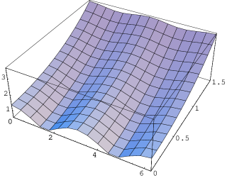
Figure 8: $Y_{3}$ as function of $\theta_{T}$ for Re$\theta_{T}=0-2\pi$ and Im$\theta_{T}=0-1.5$.

Taking determinant on Eq. (49) we know that the product of $Y_{2,3}$ is fixed by the left- and right-handed Majorana neutrino masses. The ratio of the two Yukawa couplings is determined by $\theta_{T}$. In Fig. 8 we show $Y_{3}$ as function of Re$\theta_{T}$ and Im$\theta_{T}$. Both the real and imaginary part influence the ratio between $Y_{2}$ and $Y_{3}$. Since $Y_{3}$ increases almost linearly with Im$\theta_{T}$, we expect BR($l_{i}\to l_{j}\gamma$) also increase with Im$\theta_{T}$.

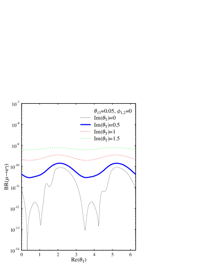
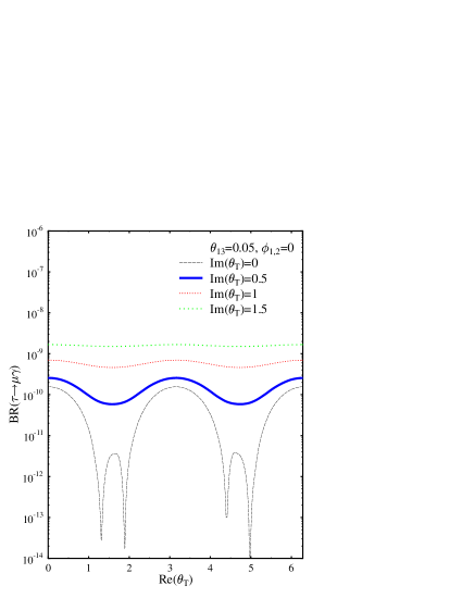
Figure 9: BR($\mu\to e\gamma$) (Left) and BR($\tau\to\mu\gamma$) (Right) as function of Re$\theta_{T}$ for Im$\theta_{T}=0,0.5,1,1.5$. We fix $\theta_{13}=0.05$, $\phi_{i}=0$ and $M_{3}=1\times 10^{15}GeV$.

In Fig. 9, we plot BR($\mu\to e\gamma$) and BR($\tau\to\mu\gamma$) as function of Re$\theta_{T}$ on the left and right panels respectively. For Im${\theta}_{T}=0.5$, BR($\mu\to e\gamma$) has been greater than the experimental limit.

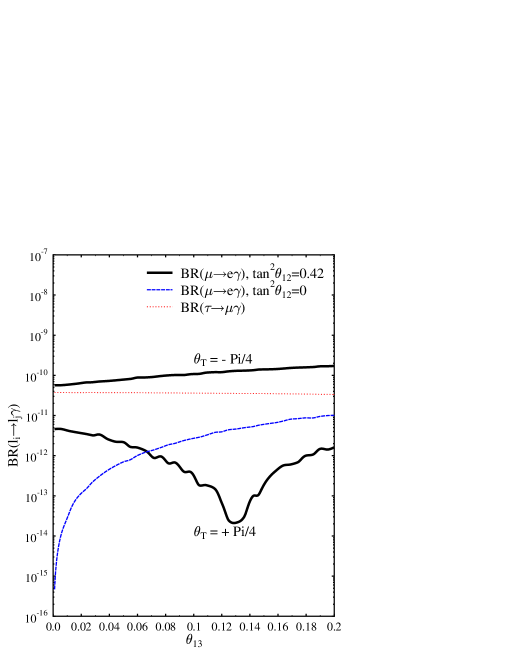
Figure 10: BR($l_{i}\to l_{j}\gamma$) as function of $\theta_{13}$. We fix $\phi_{i}=0$ and $M_{3}=1\times 10^{15}GeV$.

In Fig. 10, BR($l_{i}\to l_{j}\gamma$) is drawn as function of $\theta_{13}$. We can see BR($\mu\to e\gamma$) is very sensitive to $\theta_{13}$, while BR($\tau\to\mu\gamma$) is insensitive to $\theta_{13}$. The behavior in this figure is understood if we notice that the flavor mixing between the first and the second generations is nearly proportional to $V_{13}V_{23}^{*}Y_{3}^{2}$, where $V_{13}=(U_{\nu})_{12}V^{\prime}_{23}+(U_{\nu})_{13}V^{\prime}_{33}$. The two terms are added constructively or destructively, depending on the sign of $\theta_{T}$. When we set $\theta_{12}=0$, the branching ratio of $\mu\to e\gamma$ increases rapidly with $\theta_{13}$, independent of the value of $\theta_{T}$.

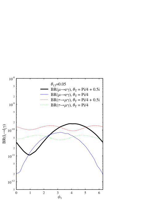
Figure 11: BR($l_{i}\to l_{j}\gamma$) as function of $\phi_{1}$. We fix $\theta_{13}=0.05$, $\phi_{2}=0$ and $M_{3}=1\times 10^{15}GeV$.

In Fig. 11, we plot BR($l_{i}\to l_{j}\gamma$) as function of $\phi_{1}$, which determines the relative phase between $U_{\nu}$ and $V^{\prime}$. The behavior in the figure is easy to understand. We also examined that BR($l_{i}\to l_{j}\gamma$) is indeed independent of $\phi_{2}$, as we expected.

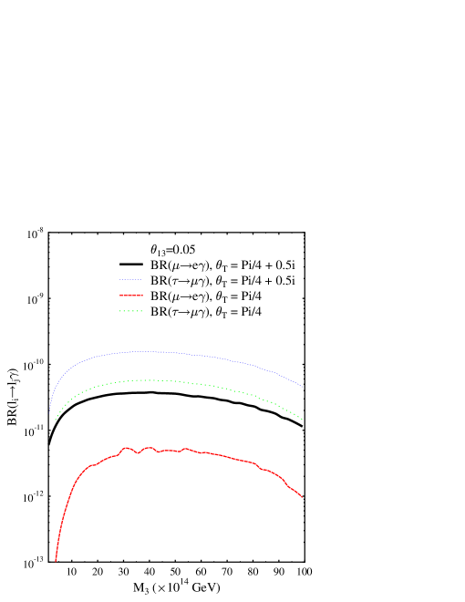
Figure 12: BR($l_{i}\to l_{j}\gamma$) as function of $M_{3}$ for $\theta_{T}=\pi/4+0.5i$ and $\theta_{T}=\pi/4$. We fix $\theta_{13}=0.05$ and $\phi_{i}=0$.

Finally, we plot BR($l_{i}\to l_{j}\gamma$) as function of $M_{3}$. BR($l_{i}\to l_{j}\gamma$) increases with $M_{3}$ at first, because it makes $Y_{2,3}$ larger. However, when $M_{3}$ is as large as $10^{16}GeV$, which is too close to $M_{GUT}$, the integration distance $\log\frac{M_{GUT}}{M_{3}}$ becomes too small and the branching ratio decreases. Although below $M_{3}$ LFV is still produced, see Eq. (40), the effects are small, since the contribution from $Y_{2}^{2}$ is small, due to $Y_{2}^{2}<<Y_{3}^{2}$. The $Y_{3}$ coupling contributes to the LFV below $M_{3}$ through the mixing, $Y_{3}^{2}|\tilde{X}_{23}|^{2}$, which is also small due to the small mixing element.

We have omitted BR($\tau\to e\gamma$) in all the figures because the predicted branching ratio is much smaller than the present experimental limit.

III.5 Neutrinoless double beta decay

From the above discussion we know that it is impossible to produce degenerate solution for the left-handed neutrino masses in this model. It is easy to estimate that $<m>_{ee}=(2\sim 4)\times 10^{-3}eV$, depending on the value of $U_{e3}$. So, in this sneutrino-inflaton model, it is hard to account for the neutrinoless double beta decay experimental signal0nubeta .

IV summary and discussions

We have considered a double-sneutrino inflation model within the minimal supersymmetric seesaw model. With the mass ratio $6\lesssim r\lesssim 10$ and the lighter sneutrino $M_{1}\sim 1.7\times 10^{13}$ GeV, the model predicts a suppressed primordial scalar spectrum around the largest scales which is favored at $>1.5\sigma$. The predicted CMB TT quadrupole is much better suppressed than the single sneutrino model and the preference level by the WMAP first year data is about $1.5\sigma$. Double quartic inflation can also work very well in light of WMAP observations.

We then have studied the phenomenological implications of this model. The seesaw parameters are constrained by both particle physics and cosmological observations. The strongest constraint comes from the required reheating temperature by the gravitino problem. To some extend, fine tunning is needed to satisfy this constraint, which means that the right-handed mixing angles $\theta_{1}$ and $\theta_{2}$ are much smaller than the mass hierarchy of the right-handed neutrinos. Further, the mass of the lightest left-handed neutrino should be at the order of $10^{-10}eV$, much smaller than the other two light neutrinos.

Leptogenesis arises from the decays of the cold inflaton— the lightest sneutrino. It is easy to account for the observed quantity of the baryon number asymmetry in the Universe by adjusting the seesaw parameters.

This model gives definite predictions on the lepton flavor violating decay rates. In most parameter space, the branching ratio of $\mu\to e\gamma$ is near or exceeds the present experimental limit. However, the branching ratio of $\tau\to\mu\gamma$ is at the order of about $10^{-10}-10^{-9}$, which is far below the current experimental limit. Furthermore, in the appropriate range of SUSY parameter space where LFV constraints are satisfied, the SUSY can only enhance the muon anomalous magnetic moment at the amount of $(2\sim 3)\times 10^{-10}$.

This model can not predict a degenerate light neutrino spectrum. The observed signal of neutrinoless double beta decay, if finally verified, can not be explained by the effective Majorana neutrino mass in this model.

- (1) A. Guth, Phys. Rev. D 23, 347 (1981); A. Linde, Phys. Lett. B 108, 389 (1982). A. Albrecht and P. J. Steinhardt, Phys. Rev. Lett. 48, 1220 (1982).
- (2) H. Murayama, H. Suzuki, T. Yanagida, and J. Yokoyama, Phys. Rev. Lett. 70, 1912 (1993); H. Murayama, H. Suzuki, T. Yanagida, and J. Yokoyama, Phys. Rev. D 50, 2356 (1994).
- (3) J. Ellis, M. Raidal and T. Yanagida, arXiv: hep-ph/0303242.
- (4) Y. Fukuda et al. [Super-Kamiokande Collaboration], Phys. Rev. Lett. 81 (1998) 1562; Q. R. Ahmad et al. [SNO Collaboration], Phys. Rev. Lett. 89 (2002) 011301, arXiv:nucl-ex/0204008; K. Eguchi et al. [KamLAND Collaboration], Phys. Rev. Lett. 90 (2003) 021802, arXiv:hep-ex/0212021.
- (5) M. Gell-Mann, P. Ramond and R. Slansky, Proceedings of the Supergravity Stony Brook Workshop, New York, 1979, eds. P. Van Nieuwenhuizen and D. Freedman (North-Holland, Amsterdam); T. Yanagida, Proceedings of the Workshop on Unified Theories and Baryon Number in the Universe, Tsukuba, Japan 1979 (eds. A. Sawada and A. Sugamoto, KEK Report No. 79-18, Tsukuba); R. N. Mohapatra and G. Senjanovic, Phys. Rev. Lett. 44, 912 (1980); S. L. Glashow, Caraese lectures, (1979).
- (6) M. Fukugita and T. Yanagida, Phys. Lett. B 174 (1986) 45; P. Langacker, R. D. Peccei and T. Yanagida, Mod. Phys. Lett. A 1, (1986) 541; R. N. Mohapatra and X. Zhang, Phys. Rev. D 46, (1992) 5331; H. Murayama and T. Yanagida, Phys. Lett. B 322 (1994) 349 arXiv:hep-ph/9310297; K. Hamaguchi, H. Murayama and T. Yanagida, Phys. Rev. D 65 (2002) 043512 arXiv:hep-ph/0109030; T. Moroi and H. Murayama, Phys. Lett. B 553 (2003) 126 arXiv:hep-ph/0211019.
- (7) C. L. Bennett et al., astro-ph/0302207.
- (8) G. Hinshaw et al., astro-ph/0302217.
- (9) C. L. Bennett et al., Astrophys. J. 464, L1 (1996).
- (10) H. V. Peiris et al., astro-ph/0302225.
- (11) W. J. Percival et al., Mon. Not. Roy. Astr. Soc. 327, 1297 (2001).
- (12) P. Mukherjee and Y. Wang, astro-ph/0303211.
- (13) S. L. Bridle, A. M. Lewis, J. Weller, and G. Efstathiou, astro-ph/0302306.
- (14) Y. Wang, D. N.Spergel, and M. A.Strauss, Astrophys.J. 510,20 1999; Y. Wang and G. Mathews, Astrophys.J. 573,1 2002; P. Mukherjee and Y. Wang, astro-ph/0301058; P. Mukherjee and Y. Wang, astro-ph/0301562.
- (15) D. N. Spergel et al., astro-ph/0302209.
- (16) J. M. Cline, P. Crotty and J. Lesgourgues, astro-ph/0304558; G. Efstathiou, astro-ph/0306431; A. d. Oliveira-Costa, M. Tegmark, M. Zaldarriaga and A. Hamilton,astro-ph/0307282; A. Niarchou, A. H. Jaffe and L. Pogosian, astro-ph/0308461.
- (17) Y.-P. Jing and L.-Z. Fang, Phys. Rev. Lett. 73,1882 (1994); J. Yokoyama, Phys. Rev. D59, 107303 (1999); S. DeDeo, R. R. Caldwell and P. J. Steinhardt, Phys.Rev.D 67, 103509 (2003) ; J. Uzan, A. Riazuelo, R. Lehoucq and J. Weeks, astro-ph/0303580 ; G. Efstathiou, Mon.Not.Roy.Astron.Soc. 343, L95 (2003); C. R. Contaldi, M. Peloso, L. Kofman, and A. Linde, JCAP 0307, 002 (2003); E. Gaztanaga, J. Wagg, T. Multamaki, A. Montana and D. H. Hughes, astro-ph/0304178; M. Kawasaki and F. Takahashi, hep-ph/0305319; M. Bastero-Gil et al., in Ref.running ; A. Lasenby and C. Doran, astro-ph/0307311; S. Tsujikawa, R. Maartens and R. Brandenberger, astro-ph/0308169; T. Moroi and T. Takahashi,astro-ph/0308208; Q. Huang and M. Li, astro-ph/0308458.
- (18) B. Feng and X. Zhang, Phys.Lett.B 570, 145 (2003)
- (19) B. Feng, M. Li, R.-J. Zhang, and X. Zhang, astro-ph/0302479.
- (20) X. Wang et al., astro-ph/0209242.
- (21) J. E. Lidsey and R. Tavakol, astro-ph/0304113; M. Kawasaki, M. Yamaguchi and J. Yokoyama, Phys.Rev. D 68, 023508 (2003); Q. G. Huang and M. Li, JHEP 0306, 014 (2003); D. J. Chung, G. Shiu and M. Trodden, astro-ph/0305193; K.-I. Izawa, hep-ph/0305286; M. Bastero-Gil, K. Freese and L. Mersini-Houghton, hep-ph/0306289; M. Yamaguchi and J. Yokoyama, hep-ph/0307373.
- (22) V. Barger, H. Lee, and D. Marfatia, Phys.Lett.B 565, 33 (2003); W. H.Kinney, E. W.Kolb, A. Melchiorri and A. Riotto, hep-ph/0305130; S. M.Leach and A. R.Liddle, astro-ph/0306305.
- (23) D. Polarski and A. A. Starobinsky, Nucl.Phys.B 385, 623 (1992); D. Polarski, Phys.Rev.D 49, 6319 (1994); D. Polarski and A. A. Starobinsky, Phys.Lett.B 356, 196 (1995); J. Lesgourgues and D. Polarski, Phys.Rev.D 56, 6425 (1997).
- (24) M. H. Kesden, M. Kamionkowski and A. Cooray, astro-ph/0306597.
- (25) M. Kamionkowski, in private communications.
- (26) J. M. Diego, P. Mazzotta and J. Silk, astro-ph/0309181; O. Dore, G. P. Holder and A. Loeb, astro-ph/0309281; P. G. Castro, M. Douspis and P. G. Ferreira, astro-ph/0309320.
- (27) J. R. Ellis, J. E. Kim and D. V. Nanopoulos, Phys. Lett. B 145 (1984) 181; J. R. Ellis, D. V. Nanopoulos and S. Sarkar, Nucl. Phys. B 259 (1985) 175; J. R. Ellis, D. V. Nanopoulos, K. A. Olive and S. J. Rey, Astropart. Phys. 4 (1996) 371; M. Kawasaki and T. Moroi, Prog. Theor. Phys. 93 (1995) 879; T. Moroi, Ph.D. thesis, arXiv:hep-ph/9503210; M. Bolz, A. Brandenburg and W. Buchmüller, Nucl. Phys. B 606 (2001) 518; R. Cyburt, J. R. Ellis, B. D. Fields and K. A. Olive, astro-ph/0211258.
- (28) H. V. Klapdor-Kleingrothaus et al., Mod. Phys. Lett. A 16, 2409 (2002).
- (29) C. Gordon, D. Wands, B.A. Bassett, and R. Maartens, Phys. Rev. D63, 023506 (2001).
- (30) S. M. Leach and A. R. Liddle, Phys. Rev. D 63, 043508 (2001); S. M. Leach, M. Sasaki, D. Wands and A. R. Liddle,Phys. Rev. D 64, 023512 (2001).
- (31) D. H. Huang, W. B. Lin and X. M. Zhang Phys. Rev. D 62, 087302 (2000).
- (32) B. Feng, X. Gong and X. Wang, astro-ph/0301111.
- (33) D. H. Lyth and A. Riotto, Phys.Rept. 314, 1 (1999).
- (34) L. Verde et al., arXiv: astro-ph/0302218.
- (35) A. R. Liddle and S. M. Leach, arXiv: astro-ph/0305263.
- (36) Z. Maki, M. Nakagawa, and S. Sakata, Prog. Theor. Phys. 28, 870 (1962).
- (37) J. A. Casas and A. Ibarra, Nucl. Phys. B 618, 171 (2001).
- (38) K. Hamaguchi, H. Murayama, T. Yanagida, Phys. Rev. D 65, 043512 (2002), arXiv: hep-ph/0109030.
- (39) W. Buchmüller, P. Di Bari and M. Plümacher, Nucl. Phys. B 643, 367 (2002).
- (40) M. L. Brooks et al., MEGA Collaboration, Phys. Rev. Lett. 83 1521 (1999); S. Ahmed et al., CLEO Collaboration, Phys. Rev. D 61 071101 (2000); U. Bellgardt et al., Nucl. Phys. B229 1 (1988).
- (41) S. Antusch, J. Kersten, M. Lindner, M. Ratz, arXiv: hep-ph/0305273.
- (42) X. J. Bi, Y. P. Kuang and Y. H. An, arXiv: hep-ph/0211142.
- (43) U. Seljak and M. Zaldarriaga, Astrophys. J. 469, 437 (1996).
- (44) http://cmbfast.org/ .