Incident-Energy Dependence of the
Effective Temperature in Heavy-Ion Collisions

I Introduction

Experimental data on transversal momentum distributions of kaons produced in central Pb+Pb or Au+Au collisions show an anomalous dependence on the collision energy ags ; sps ; rhic . The effective temperature $T^{*}$, or slope parameter of the transversal-momentum spectra note1 , increases with energy in AGS and RHIC energy domains. However, in the SPS energies the effective temperature keeps approximately constant. Recently, it was argued MG2a that this behaviour might be caused by a modification of the equation of state in the transition region between confined and deconfined matter, as suggested by Van Hove Hov a long time ago, and could be considered as new signal of deconfinement in the SPS energy domain.

Our main object in the present work is to study the behaviour of the effective temperature for K⁺ in several energy domains. For this purpose, we apply the recently developed SPheRIO Aguiar2001 ; Aguiar2002 code for hydrodynamics in 3+1 dimensions, using both Landau-type compact initial conditions and spatially more spread ones. For the latter we used the average over many events generated by NeXus nexus1 ; nexus2 . We show that initial conditions given in small volume, like Landau-type ones, are unable to reproduce the effective temperature together with other data (multiplicities and rapidity distributions). These quantities can be reproduced altogether only when using a large initial volume with an appropriate velocity distribution.

Besides, it seems that the increase of $T^{*}$ in the RHIC energy domains is caused mainly by the larger expansion time in the hadronic phase for higher incidente energy, which implies lower freeze-out temperature as $\sqrt{s}$ increases HN ; NNOP . It seems that, within our analyses with NeXus initial conditions, the RHIC incident energies are not enough to produce noticeable increase in the transverse acceleration during the quark-gluon plasma (QGP) phase.

II Hydrodynamics in 3+1 dimensions

The hydrodynamical code in 3+1 dimensions used here is based on the technique called Smoothed Particle Hydrodynamics (SPH) Lucy1977 ; Gingold1977 . This is a method which uses Lagrangian coordinates. The fluid is represented by small volumes called SPH-particles and the equations for the fluid evolution become a system of ordinary differencial equations for the SPH-particles, in this representation.

The numerical code SPheRIO note2 is a suitable implementation of this method for the relativistic nuclear collisions. An advantage of this technique is the convenience in the study of problems where the geometry is highly irregular, as is the case of non-central relativistic collisions. A SPH-particle has attached to it conserved quantities; in the present version of SPheRIO, the entropy and the baryonic number are the quantities which are kept constant during the fluid evolution. In the SPH representation, the entropy density and the baryonic density are parametrized as:

$$s(\tau,\bm{x}) = \frac{1}{\tau\gamma}\sum_{i}\nu_{i}^{s}W(\bm{x}-\bm{x}_{i};h),$$ (1)

$$n_{b}(\tau,\bm{x}) = \frac{1}{\tau\gamma}\sum_{i}\nu_{i}^{b}W(\bm{x}-\bm{x}_{i};h),$$ (2)

where $\nu_{i}^{s}$ ($\nu_{i}^{b}$) is the entropy (baryonic number) of the $i$-th SPH-particle, $\gamma=1/\surd(1-v_{x}^{2}-v_{y}^{2}-\tau^{2}v_{\eta}^{2})$, and $W$ is the interpolating kernel with width $h$. Here we use the hyperbolic coordinates $\tau\equiv\surd{(t^{2}-z^{2})}$, $x$, $y$ and $\eta\equiv 1/2\cdot\ln[(t+z)/(t-z)]$ which are convenient for a system in rapid longitudinal expansion. The equations for the SPH-particles are given by:

$$\frac{d\bm{x}_{i}}{d\tau} = \bm{v}_{i},$$ (3)

$$\frac{d}{d\tau}\left(\gamma\nu^{s}\;\frac{P+\varepsilon}{s}\;\bm{\omega}\right)_{i} = -\sum_{j}\nu_{i}^{s}\nu_{j}^{s}\left[\frac{P_{i}}{\tau\gamma_{i}^{2}s_{i}^{2}}+\frac{P_{j}}{\tau\gamma_{j}^{2}s_{j}^{2}}\right]\bm{\nabla}_{i}W(\bm{x}_{i}-\bm{x}_{j};h),$$ (4)

where $\bm{\omega}=(v_{x},v_{y},\tau^{2}v_{\eta})$. The pressure, $P$, and the energy density, $\varepsilon$, are related to the entropy density $s$ and the baryonic density $n_{b}$ via equation of state.

II.1 Decoupling criterion

The distribution of final particles is obtained by using Cooper-Frye’s prescription CF :

$$E\frac{d^{3}N}{dp^{3}}=\int_{\Sigma_{fo}}d\sigma\cdot pf(p\cdot u),$$ (5)

where $f(p\cdot u)$ is the distribution function (Bose-Einstein or Fermi-Dirac) and the integral is evaluated on the freeze-out surface $\Sigma_{fo}$. In the SPH representation, Eq. (5) is written as

$$E\frac{d^{3}N}{dp^{3}}=\sum_{i}\frac{\nu_{i}^{s}\;\hat{n}_{i}\cdot p}{s_{i}\;|\hat{n}_{i}\cdot u_{i}|}f(p\cdot u_{i}),$$ (6)

where the sum is over all SPH-particles on the freeze-out surface and $\hat{n}$ is the normal four-vector to this surface, given by $\hat{n}_{\mu}\propto(-\partial T/\partial\tau,-\partial T/\partial x,-\partial T/\partial y,-\partial T/\partial\eta)$.

III Equations of state

Let us consider here two sets of equations of state. The first one type-I (EOS-I) has a first-order phase transition between an ideal gas of massless quarks (u, d and s) and gluons and an ideal hadron gas (baryon number is assumed to be zero), where the pressure, the energy density and the entropy density are given by:

$$P_{q} = \frac{\pi^{2}}{90}g_{q}T^{4}-B,$$ (7)

$$\varepsilon_{q} = \frac{\pi^{2}}{30}g_{q}T^{4}+B,$$ (8)

$$s_{q} = \frac{2\pi^{2}}{45}g_{q}T^{3},$$ (9)

$$P_{h} = \frac{\pi^{2}}{90}g_{h}T^{4},$$ (10)

$$\varepsilon_{h} = \frac{\pi^{2}}{30}g_{h}T^{4},$$ (11)

$$s_{h} = \frac{2\pi^{2}}{45}g_{h}T^{3}.$$ (12)

Here $g_{h}=16$ is an effective parameter (see MG2b for details), $g_{q}=95/2$, and $B$ is the bag model parameter.

The second one, type-II (EOS-II), somewhat more realistic than the previous one, considers a first-order phase transition between a QGP and a hadronic resonance gas (baryon number is taking into account). In the QGP we consider an ideal gas of massless quarks (u, d, s) and gluons. The thermodynamical quantities are given by

$$P_{q} = \frac{\pi^{2}}{90}g_{q}T^{4}+\frac{3}{2}\left(T^{2}\mu_{q}^{2}+\frac{\mu_{q}^{4}}{2\pi^{2}}\right)-B,$$ (13)

$$\varepsilon_{q} = \frac{\pi^{2}}{30}g_{q}T^{4}+\frac{9}{2}\left(T^{2}\mu_{q}^{2}+\frac{\mu_{q}^{4}}{2\pi^{2}}\right)+B,$$ (14)

$$s_{q} = \frac{2\pi^{2}}{45}g_{q}T^{3}+3T\mu_{q}^{2},$$ (15)

$$n_{q} = 3\left(T^{2}\mu_{q}^{2}+\frac{\mu_{q}^{3}}{\pi^{2}}\right).$$ (16)

The hadronic phase is composed of resonances with mass below 2.5 GeV/c², where volume correction is taken into account. The corrected-volume pressure, $P^{ex}$, is written in function of the pressure for an ideal gas $P^{id}$:

$$\sum_{i}P_{i}^{ex}(T,\mu_{i})=\sum_{i}P_{i}^{id}(T,\tilde{\mu}_{i}),$$ (17)

where $\tilde{\mu}_{i}=\mu_{i}-V_{i}\sum_{j}P_{j}^{id}(T,\tilde{\mu}_{j})$, ($V_{i}$: volume of the hadron $i$). Others thermodynamical quantities are given following the relation:

$$\chi_{i}^{ex}(T,\mu_{i})=\frac{\chi_{i}^{id}(T,\tilde{\mu}_{i})}{1+\sum_{j}V_{j}n_{j}^{id}(T,\tilde{\mu}_{j})},$$ (18)

where $\chi$ represents $n$, $\varepsilon$ or $s$.

In both equations of state, the transition temperature is assumed to be 160 MeV.

IV Initial conditions and results

In order to study the behaviour of the effective temperature, we began with Landau-type initial conditions, where the fluid is at rest at $t=0$ fm/c, and the matter is localized in a Lorentz contracted sphere. The initial energy density is assumed to be constant and given by: $\varepsilon_{0}=E/V$, where $E=\zeta(\sqrt{s}-2m)A$ is the available kinetical energy in the collision, and $V=\gamma_{0}^{-1}V_{0}=\gamma_{0}^{-1}(4/3)\pi R^{3}$ is the volume of the contracted incident nuclei when superposed. Here $\zeta$ is the inelasticity parameter and $\gamma_{0}=\sqrt{s}/2m$. These initial conditions (together with EOS-I) can reproduce both the particle multiplicities and the rapidity distributions fairly well (Ref. MG2b ). However it has an inconvenience that the initial energy density is too high. As a consequence, the time of expansion becomes very large and transverse expansion is considerable. The result is a very large effective temperature and a non-exponential shape of the spectra in transverse momentum.

A solution we found to this problem was to give the fluid an initial longitudinal-velocity distribution. We did not change the shape of the region where the fluid is formed, which remained a Lorentz contracted sphere. The initial longitudinal velocity is not constant, but proportional to $z$:

$$u^{\mu}(z) = (\gamma(z),0,0,\gamma(z)v),$$ (19)

$$u^{z}(z) = \frac{z}{z_{m}}\,\zeta\sqrt{\gamma_{0}^{2}-1},$$ (20)

$$\gamma(z) = \sqrt{\left(\frac{z}{z_{m}}\right)^{2}\zeta^{2}(\gamma_{0}^{2}-1)+1},$$ (21)

where $z_{m}=R/\gamma_{0}$. As a consequence of this change, the initial energy density $\varepsilon_{0}$, which we took constant and obtained solving the equation

$$E=\int\limits_{V:\;\;r^{2}+\gamma_{0}^{2}z^{2}=R^{2}}\left[(\varepsilon_{0}+p)\gamma^{2}(z)-p\right]dV,$$ (22)

became much smaller and then the transverse expansion compatible with data, as shown in Table 1 and Fig. 1. In this simulation we consider freeze-out temperatures smoothly increasing with energy, until SPS domains. For RHIC energies, we show two cases: a decreasing freeze-out temperature and a increasing one (bold-faced types in Table 1 and triangle in Fig. 1).

However, since $\varepsilon_{0}$ became much smaller than the previous case, so did the entropy density $s_{0}$ and the total multiplicity, although the rapidity distributions remained more or less the same in the shape.

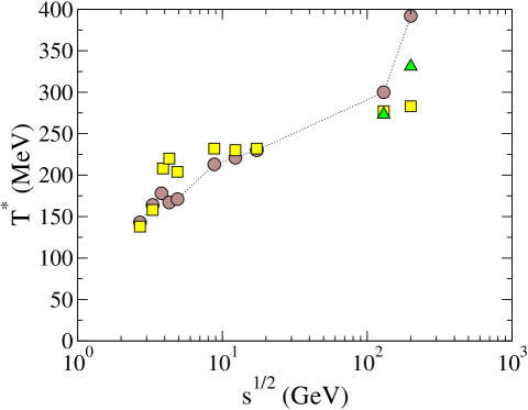
Figure 1: Energy dependence of the effective temperature for K⁺. The initial conditions are Landau-type ones, with initial longitudinal velocity. Triangles corresponde to $T_{fo}$=155 MeV. Experimental data are shown in square symbols.

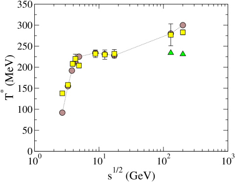
Figure 2: Energy dependence of the effective temperature for K⁺. The initial conditions are NeXus-type ones. Triangles corresponde to $T_{fo}$=155 MeV. Experimental data are shown in square symbols.

To reproduce all quantities (multiplicities, rapidity distributions and transverse-momentum distributions) we have to take a large initial volume, with some appropriate longitudinal-velocity distribution. To do this, we use the NeXus event generator, which produces the event-by-event initial conditions at time $\tau=1$ fm/c. Instead of using these fluctuating initial conditions, here we smooth them out by averaging 30 random events for each collision energy. For this case we use the EOS-II. The results are shown in Table 2 and Fig. 2. Besides reproducing the effective temperature data quite well, it was shown that this initial conditions give good results also of multiplicity and rapidity distributions HGSAKPTO .

Table 1: Results obtained from Landau-type initial conditions with initial longitudinal velocity. $\bar{v}_{T}$ is the transversal velocity averaged in the rapidity interval $-0.5\leq y\leq 0.5$. $\varepsilon_{0}$ is the initial energy density and $T_{0}$ is the corresponding initial temperature.

$\sqrt{s}$	$T_{0}$	$\varepsilon_{0}$	$T_{fo}$	$\bar{v}_{T}$	$T^{*}$
(A$\cdot$GeV)	(MeV)	(GeV/fm3)	(MeV)		(MeV)
2.7	109	0.097	85	0.240	143
3.3	128	0.185	94	0.255	164
3.8	140	0.263	97	0.280	178
4.3	149	0.341	115	0.155	167
4.9	158	0.431	120	0.153	171
8.8	160	1.038	143	0.146	213
12.3	160	1.322	147	0.147	221
17.3	160	1.536	149	0.139	230
130	167	1.896	128	0.292	300
			155	0.191	273
200	168	1.908	125	0.485	392
			155	0.272	331

Table 2: Results obtained from NeXus-type initial conditions. The initial energy density $\varepsilon_{0}$ and the initial temperature $T_{0}$ are given in the central point ($x=y=\eta=0$). $\bar{v}_{T}$ is the transversal velocity averaged in the rapidity interval $-0.5\leq y\leq 0.5$.

$\sqrt{s}$	$T_{0}$	$\varepsilon_{0}$	$T_{fo}$	$\bar{v}_{T}$	$T^{*}$
(A$\cdot$GeV)	(MeV)	(GeV/fm3)	(MeV)		(MeV)
2.7	98	0.75	85	0.067	92
3.3	128	0.66	94	0.28	155
3.8	131	1.01	97	0.41	192
4.3	135	1.38	115	0.37	212
4.9	140	1.55	120	0.39	225
8.8	198	4.06	143	0.32	234
12.3	248	9.04	147	0.32	231
17.3	265	11.37	149	0.32	228
130	279	12.86	128	0.52	280
			155	0.34	234
200	277	12.48	125	0.56	300
			155	0.34	231

V Conclusions

We conclude that the initial conditions given in small volume like Landau-type discussed above are not appropriated to describe the multiplicity data, rapidity distributions and the transverse-momentum distributions at the same time. If we try to obtain the correct multiplicities (together with the rapidity distributions), the effective temperature becomes too large (the first case discussed in Sec. IV, where the fluid is at rest) . On the other side, if we try to get the correct effective temperature and the shape of rapidity distributions as we did, the multiplicities become small, unless an additional entropy is generated during the expansion (the second case discussed in Sec. IV). It is clear that these conclusions about the initial conditions do not change if we replace EOS-I by EOS-II.

Nexus type initial conditions, with spatially spread energy and velocity distributions, reproduce well all the main characteristics of data, namely particle multiplicities, rapidity distributions and $p_{T}$ spectra. In this case, the increase of $T^{*}$ in RHIC energy domain seems to be due mostly to the larger expansion in the hadronic phase than to that in the QGP phase.

References

- (1) L. Ahle et al., Phys. Lett. B490, 53 (2000).
- (2) S. V. Afanasiev et al., Phys. Rev. C66, 054902 (2002).
- (3) D. Ouerdane et al., nucl-ex/0212001; C. Adler et al., nucl-ex/0206008.
- (4) The effective temperature, , is obtained by fitting the transverse-mass distribution with the function .
- (5) M. I. Gorenstein, M. Gaździcki and K. A. Bugaev, hep-ph/0303041.
- (6) L. Van Hove, Phys. Lett. B118, 138 (1982).
- (7) C. E. Aguiar, Y. Hama, T. Kodama and T. Osada, J. Phys. G27, 75 (2001).
- (8) C. E. Aguiar, Y. Hama, T. Kodama and T. Osada, Nucl. Phys. A698, 639c (2002).
- (9) H. J. Drescher, M. Hladik, S. Ostapchenko, T. Pierog and K. Werner, Phys. Rep. 350, 93 (2001).
- (10) H. J. Drescher, F. M. Liu, S. Ostapchenko, T. Pierog and K. Werner, Phys. Rev. C65, 054902 (2002).
- (11) Y. Hama and F. S. Navarra, Z. Phys. C53, 501 (1992).
- (12) F. S. Navarra, M. C. Nemes, U. Ornik and S. M. Paiva, Phys. Rev. C45, R2552(1992).
- (13) L. B. Lucy, Astrophys. J. 82, 1013 (1977).
- (14) R. A. Gingold and J. J. Monaghan, Mon. Not. R. Astron. 181, 375 (1977).
- (15) Smoothed Particle hydrodynamical evolution of Relativistic heavy IOn collisions.
- (16) F. Cooper and G. Frye, Phys. Rev. D10, 186 (1974).
- (17) M. Gaździcki and M. I. Gorenstein, Acta Phys. Polon. B30, 2705 (1999).
- (18) Y. Hama, F. Grassi, O. Socolowski Jr., C. E. Aguiar, T. Kodama, L. L. S. Portugal, B. M. Tavares and T. Osada, Event-by-Event Fluctuation of the Initial Conditions in Hydrodynamical Model, presented to 32nd. Int. Sym. on Multiparticle Dynamics, Alushta (Ukraine), Sep 7-13, 2002.