Evidence for Solar Neutrino Flux Variability and its Implications

Abstract

Although KamLAND apparently rules out Resonant-Spin-Flavor-Precession (RSFP) as an explanation of the solar neutrino deficit, the solar neutrino fluxes in the Cl and Ga experiments appear to vary with solar rotation. Added to this evidence, summarized here, a power spectrum analysis of the Super-Kamiokande data reveals significant variation in the flux matching a dominant rotation rate observed in the solar magnetic field in the same time period. Three frequency peaks, all related to this rotation rate, can be explained quantitatively. A Super-Kamiokande paper reported no time variation of the flux, but showed the same peaks, there interpreted as statistically insignificant, due to an inappropriate analysis. This modulation is small (7%) in the Super-Kamiokande energy region (and below the sensitivity of the Super-Kamiokande analysis) and is consistent with RSFP as a subdominant neutrino process in the convection zone. The data display effects that correspond to solar-cycle changes in the magnetic field, typical of the convection zone. This subdominant process requires new physics: a large neutrino transition magnetic moment and a light sterile neutrino, since an effect of this amplitude occurring in the convection zone cannot be achieved with the three known neutrinos. It does, however, resolve current problems in providing fits to all experimental estimates of the mean neutrino flux, and is compatible with the extensive evidence for solar neutrino flux variability.

1 Introduction

Results from the KamLAND experiment [1] seem to confirm the Large-Mixing Angle (LMA) solution to the solar neutrino deficit and rule out the Resonant-Spin-Flavor-Precession (RSFP) explanation [2]. On the other hand, there is increasing evidence [3, 4, 5, 6, 7, 8, 9, 10] that the solar neutrino flux is not constant as assumed for the LMA solution, but varies with periods that can be attributed to well-known solar processes. This suggests that the solar neutrino situation may be more complex than is usually assumed, and that RSFP may be subdominant to LMA [11, 12], requiring a large transition magnetic moment and hence new physics. Since this recent information on solar neutrino variability is not widely known, a brief summary is presented here of analyses of radiochemical neutrino data, along with newer input from the Super-Kamiokande experiment [13]. Although the 10-day averages of Super-Kamiokande solar neutrino data [14] show no obvious time dependence, power-spectrum analyses [15, 16, 17] displayed a strong peak at the frequency $26.57\pm 0.05$ y^-1 (period 13.75 d), as well as one at 9.42 y^-1. These were clearly an alias pair, due to the extremely regular 10-day binning for which the timing had a strong periodicity with frequency 35.99 y^-1 ($=26.57+9.42$). A subsequent Super-Kamiokande paper [18] provided 5-day averages of the data, and there was no longer evidence for the 26.57 y^-1 peak, showing it to be an alias of the 9.42 y^-1 peak (which will be explained later) due to the extremely regular 10-day binning. In the 5-day data the 9.42 y^-1 is enhanced. We also find a peak at 39.28 y^-1, which is the frequency of a dominant rotation-related oscillation in the photospheric magnetic field. Another notable peak at 43.72 y^-1 may be attributed to the same physical process as that responsible for the peak at 9.42 y^-1.

A suggested subdominant process that is compatible with these periodicities involves an RSFP transition in which the solar $\nu_{e}$ changes to a different flavor, and the spin is flipped. As in the MSW process [19], this can occur resonantly at an appropriate solar density. The two processes, LMA MSW and RSFP, would take place sequentially at different solar radii. If the RSFP process were to be achieved with the three known active neutrinos, their measured mass differences would require that RSFP occurs at a smaller solar radius than that at which the MSW effect takes place, placing it in the solar core. This case has been analyzed [12], with the result that the flux modulation produced by RSFP is very small, varying with neutrino energy from 0.8% at 2.5 MeV to 4% at 13 MeV for a product of field and magnetic moment of $10^{-6}$G$\mu_{B}$.

Another model was suggested in an earlier version of this paper, and predictions from it have been calculated [11]. This model utilizes a sterile neutrino that couples to the electron neutrino only through a transition magnetic moment. The lack of mixing with active neutrinos avoids all known limitations on sterile neutrinos, and the sterile final-state also makes irrelevant the usual constraints on RSFP from the null observations of solar antineutrinos. The solar data require a mass-squared difference between the electron and sterile neutrinos of $\Delta m^{2}\sim 10^{-8}$ eV². This is different from the mechanism and the sterile state suggested by de Holanda and Smirnov [20] for a subdominant transition to improve agreement with the Homestake data [21] and the Super-Kamiokande energy dependence [13], but again a decided improvement in the fit to the solar neutrino data is obtained [11]. This improvement, and also the reason RSFP by itself actually provides a better fit to mean solar data than does LMA [22, 23], results from the shape of the RSFP neutrino survival probability. It has a resonance pit at a density that suppresses the 0.86 MeV ⁷Be line (as does the Small-Mixing Angle [SMA] solution), but tends toward 1/2 and hence fits the Super-Kamiokande spectrum, whereas the survival probability goes to unity in the SMA case. The high-energy rise includes the neutral current scattering of the products of the spin-flavor flips, which need to be active, and hence Majorana neutrinos are required in order to fit [23] the SNO data [24] for RSFP by itself. In the case of subdominant RSFP, the high-energy behavior is determined mainly by the MSW transition, since the observed flux modulation is found to be small ($\sim 7$%) in the ⁸B neutrino region. Going down to intermediate energies, the dip toward the resonance pit reduces the predicted rate for the Homestake experiment [21], improving agreement with the data, and eliminates the rise below $\sim 8$ MeV which is predicted by the LMA solution but not observed by Super-Kamiokande [13] or SNO [24]. The electron-neutrino-associated sterile neutrino, which provides a better fit to the solar data and is required for this version of subdominant RSFP, is different from the muon-neutrino-associated sterile neutrino needed for the results of the LSND experiment [25]. Possibly three sterile neutrinos exist with a family symmetry.

2 Review of Past Evidence

The three-neutrino and four-neutrino RSFP models discussed above differ in their predictions of the location of the RSFP process in the Sun and in the size of the flux modulation they produce. The modulation is larger in the case with the added sterile neutrino, and the modulation can increase at smaller energies [11], the reverse of the other model. These distinctions should be kept in mind as the previously published evidence for solar neutrino flux variability is reviewed briefly.

By analyzing $10^{3}$ simulated data sequences, it was found [3] that the variance of the Homestake solar neutrino data [21] is larger than expected at the 99.9% confidence level (CL). A power spectrum analysis [3] of the data showed a peak at $12.88\pm 0.02$ y^-1 (28.4 d), compatible with the rotation rate of the solar radiative zone. Peak widths are computed for a probability drop to 10%. A lower limit to the width of a peak is set by the duration of the time series—in this case 24 y, so that the power spectrum analysis should be able to resolve peaks with separation as small as 0.04 y^-1. Four sidebands to the 12.88 y^-1 frequency gave evidence at the 99.8% CL for a latitudinal effect associated with the tilt of the sun’s rotation axis, and the latitude dependence was also seen directly in the data at the 98% CL [4].

The GALLEX data [26] showed a peak at $13.59\pm 0.04$ y^-1, compatible with the equatorial rotation rate of the deep convection zone [7, 8]. This peak is also in the Homestake data, and a combined analysis of both datasets shows that the 13.59 y^-1 peak is stronger than in either dataset alone. Comparison [7] of the power spectrum for the GALLEX data with a probability distribution function for the solar synodic rotation frequency as a function of radius and latitude, derived from SOHO/MDI helioseismology data [27], results in Fig. 1. This map shows that the rotation frequency matches the neutrino modulation in the equatorial section of the convection zone at about 0.8 of the solar radius, $R_{\odot}$. Note that this is compatible with the RSFP model that involves a sterile neutrino, but not with the three-neutrino model.

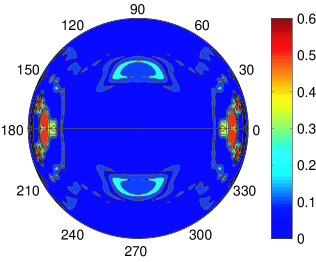
Figure 1: Map of the resonance statistic of the SOHO/MDI helioseismology and GALLEX data on a meridional section of the solar interior. The only high probability areas (red) are lens-shaped sections near the equator, and all others are low probability.

The influence of these rotation frequencies extends even to the corona, since the SXT instrument [28] on the Yohkoh spacecraft provides X-ray evidence for two “rigid” rotation rates, one ($13.55\pm 0.02$ y^-1) mainly at the equator, and the other ($12.86\pm 0.02$ y^-1) mainly at high latitudes. These values are in remarkable agreement [8] with the neutrino modulation frequencies and also with their equatorial location in one case and non-equatorial in the other; see Fig. 2. A plausible interpretation of this result is that a large-scale magnetic structure deep in the convection zone modulates the neutrino flux and is also responsible for the structure of the low-$k$ component of the photospheric magnetic field (where $k$ is wave-number), and that the coronal magnetic field reflects the low-$k$ components rather than the high-$k$ components that arise from granulation.

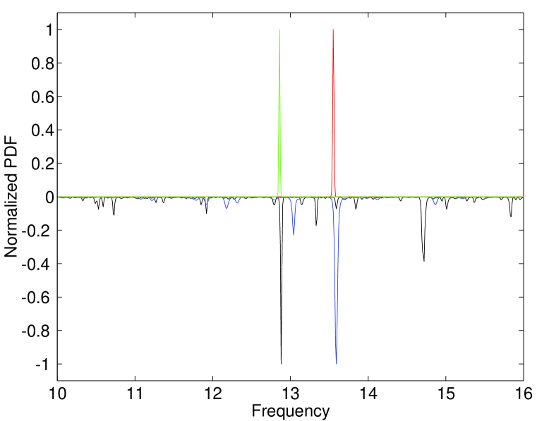
Figure 2: Comparison of normalized probability distribution functions formed from power spectra of data from SXT equator (red), SXT N60-S60 (green), Homestake (black), and GALLEX (blue). Note that the SXT (red) and GALLEX data are equatorial, and the other two are not. In this and all subsequent figures frequencies are in cycles per year.

The fact that coronal X-rays and the neutrino flux both show evidence of two dominant rotation frequencies is quite consistent with similar results of analyses of other solar variables. For instance, an analysis [29] of the photospheric magnetic field during solar cycle 21 found two dominant magnetic regions: one in the northern hemisphere with synodic rotation frequency $\sim 13.6$ y^-1, and the other in the southern hemisphere with synodic rotation frequency $\sim 13.0$ y^-1. Similarly, an analysis [30] of flares during solar cycle 23 found a dominant synodic frequency of $\sim 13.5$ y^-1 for the northern hemisphere and $\sim 12.9$ y^-1 for the southern hemisphere. These and other studies show a strong tendency for magnetic structures to rotate either at about 12.9 y^-1 or at about 13.6 y^-1. Since the Sun’s magnetic field is believed to originate in a dynamo process at or near the tachocline, it is possible that some magnetic flux is anchored in the radiative zone just below the tachocline, where the synodic rotation frequency is about 12.9 y^-1, and some just above the tachocline in the convection zone, where the synodic rotation frequency is about 13.6 y^-1. It is also possible that the 12.9 y^-1 frequency results from a latitudinal wave motion in the convection zone excited by structures at or near the tachocline.

An example of latitudinal oscillatory motion of magnetic structures may be the well-known Rieger-type oscillations (seen in gamma-ray flares, sunspots, etc.) with frequencies of about 2.4, 4.7, and 7.1 y^-1 [31]. These periodicities may be attributed to r-mode oscillations [33] with spherical harmonic indices $\ell=3$, $m=1$,2,3, giving frequencies $\nu=2m\nu_{R}/\ell(\ell+1)$, where $\nu_{R}$ is the sidereal rotation rate $[\nu({\rm sid})=\nu({\rm syn})+1]$. These frequencies are also seen in neutrino data [3, 5]. A joint spectrum analysis [10] of Homestake and GALLEX-GNO data yields peaks at 12.88, 2.33, 4.62, and 6.94 y^-1, indicating a sidereal rotation frequency $\nu_{R}=13.88\pm 0.03$ y^-1. These r-mode frequencies provide further, and somewhat unexpected, evidence for neutrino flux variations, and we return later to another observation of them.

3 Observations in the Neutrino Context

The difference between the main modulations detected by the Cl and Ga experiments may be explained by the tilt of the solar axis relative to the ecliptic, along with the fact that Cl and Ga neutrinos are produced mainly at quite different radii. The Ga data come mostly—especially in the sterile-neutrino model, where the fit requires suppressing the ⁷Be line—from $pp$ neutrinos, which originate predominantly at large solar radius ($\sim 0.2$ R_⊙), so that the wide beam of neutrinos detected on Earth is insensitive to axis tilt. Thus the beam of neutrinos detected by the Ga experiments exhibits no seasonal variation and can be modulated by the equatorial structure indicated in Fig. 1, leading to the observed frequency at about 13.6 y^-1. On the other hand, the Homestake experiment detects neutrinos produced from a smaller sphere ($\sim 0.05$ R_⊙), so that the axis tilt may cause these neutrinos mainly to miss the equatorial structure of Fig. 1 and instead sample nonzero latitudes where the 12.9 y^-1 modulation may be more significant. Twice a year, axis tilt has no effect for these neutrinos, leading to a seasonal variation in the measured flux [4].

In the sterile-neutrino model, the 13.6 y^-1 frequency, located as in Fig. 1, represents a modulation of the $pp$ neutrinos which are at or near the steeply falling edge of the neutrino survival probability as it dips toward the RSFP resonance pit. This pit, which suppresses the ${}^{7}\rm{Be}$ neutrinos, is where the largest value of the mass-squared difference between the initial and final states, divided by their energy, satisfies

$$\Delta m^{2}/E=2\sqrt{2}G_{F}N_{\rm eff},$$ (1)

and is essentially the same as for an MSW resonance [19], since it also arises from a difference in forward-scattering amplitudes of the two states. Ignoring angle factors, for MSW $N_{\rm eff}=N_{e}$ (the electron density), and for RSFP and active-active transitions, $N_{\rm eff}=N_{e}-N_{n}$ for Majorana neutrinos, where $N_{n}$ is the neutron density (about $N_{e}/6$ in the region of interest in the Sun). For Dirac neutrinos $N_{\rm eff}=N_{e}-N_{n}/2$, but for RSFP alone (not the subdominant case), only Majorana neutrinos fit all the solar data. For the more complicated subdominant case involving a transition magnetic moment coupling to a sterile state, the numerical result of Ref. [11] may be used. It shows the resonant transition occurring close to 0.8 R_⊙ for $\Delta m^{2}=1.8\times 10^{-8}$ eV², which provides a good fit to the data. This result is in remarkable agreement with the position shown in Fig. 1.

4 Changes with Solar Cycle

It is well known that the convection zone magnetic field changes with the solar cycle, so the neutrino modulation features described above should not be permanent in the sterile-neutrino model. It has been argued [34] that an RSFP effect would have to be in the radiative zone (the location of the RSFP in the three-neutrino model), where the field does not change with the solar cycle, on the assumption that solar cycle variations are not manifested. On the contrary, we show here that solar cycle changes play an important role. Variations in neutrino rates are difficult to observe, since changes in field magnitude would be undetectable if the transition remains adiabatic, and even if flux modulation results, average rates may vary only slightly.

In the sterile-neutrino model the feature that is most sensitive to field magnitude or radial variation is the intersection of the very steeply falling $pp$ neutrino spectrum with the edge of the RSFP resonance pit. The shape of the neutrino transition probability function depends not only on the resonance location, Eq. (1), but also on the product of the magnetic moment and magnetic field strength. Thus a change in field will shift the intersection of the $pp$ spectrum and resonant pit edge and change the degree of modulation. As can be seen in Fig. 3, the peak at 13.6 y^-1 associated with these neutrinos increased in strength from the start of data taking after the solar maximum of 1989.6 to the solar minimum of 1996.8, after which the modulation becomes weak. Also it was during that cycle that the main buildup in the strength of the 12.9 y^-1 oscillation was detected by Homestake. The SXT X-ray data, with which these two frequencies have remarkable agreement [8], also came from that same solar cycle.

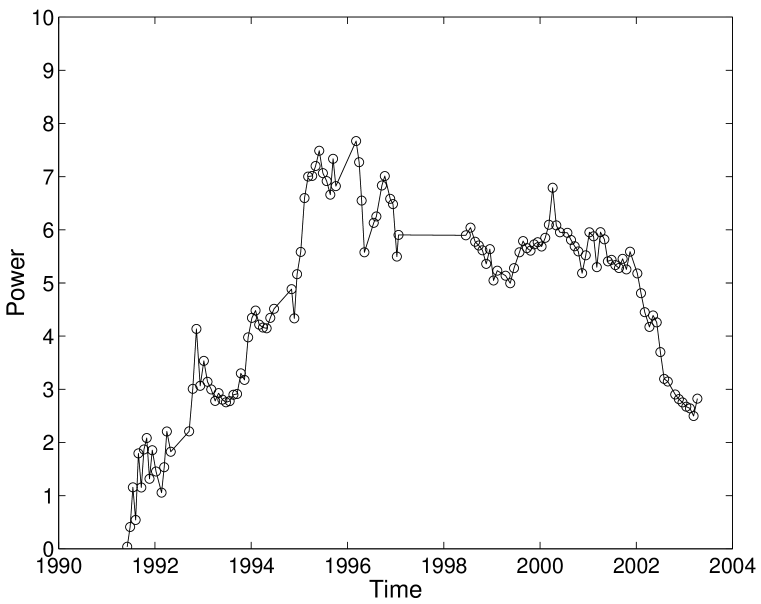
Figure 3: Running Rayleigh power, as a function of end time, for frequency 13.59 y^-1 from the GALLEX-GNO data. Note that the power builds up from the start of data taking after the 1990 solar maximum until the 1996.8 solar minimum, after which there is little evidence for that frequency.

In response to a paper [35] suggesting that the 13.59 y^-1 line is not statistically significant in the GALLEX-GNO data, we have recently shown [36] that the difference is due to different choices made in the analysis procedures, such as whether or not one takes into account solar cycle changes. Using the most sensitive analysis choices, we found the 13.59 y^-1 modulation to be significant at the 99.9% confidence level.

Another feature one may attribute to a time variation of the intersection of the $pp$ spectrum with the edge of the RSFP resonance pit is the appearance [6] of a bimodal flux distribution in the Ga data, as shown in Fig. 4. A single peak would be expected if there were no flux modulation. This structure is clearly evident in unbinned data during the same solar maximum to solar minimum period. This neutrino flux effect also diminishes after the solar minimum. Adding to the significance of this result is the plot of Fig. 5, which shows that when the end times of runs are reordered according to the phase of the 13.59 y^-1 rotation, the flux values are low in one-half of the cycle and high in the other.

Figure 4: Histogram of GALLEX data. The arrow indicates the maximum-likelihood estimate of the flux (in SNU).

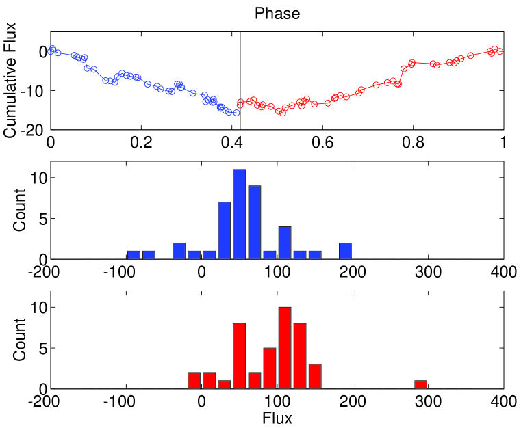
Figure 5: Normalized GALLEX flux (in SNUs) measurement runs (prior to 1997) reordered according to the phase of the 13.59 y^-1 solar modulation. The division in phase is made so as to have equal numbers of events in the descending (blue) and ascending (red) parts of the cycle.

It is unfortunate that the Homestake experiment, which detected mainly the ⁸B neutrinos (the only neutrino component registered by Super-Kamiokande) ceased operation before Super-Kamiokande started. As a result, there is no way to predict from other solar neutrino experiments what neutrino flux variation should have been detected by Super-Kamiokande during its operation from May 1996 (near solar minimum) until July 2001 (near solar maximum). However, it is possible to compare Super-Kamiokande measurements with other solar variables that reflect the influence of the Sun’s internal magnetic field. It is important to emphasize that the change in the solar field at a change in solar cycle makes it impossible to predict, even for the same experiment, what modulation frequencies will be observed in a new solar cycle if one has data only from previous solar cycles. This would not be true for the three-neutrino model for which the RSFP process is located in the stable radiative zone.

5 Super-Kamiokande Data Analysis

The Super-Kamiokande group released [14] flux measurements in 184 bins of about 10 days each. The flux measurements vary over the range $2:1$, and the fractional error of the measurement (averaged over all bins) is $0.14$. Because of the regularity of the binning, the “window spectrum” (the power spectrum of the acquisition times) has a huge peak (power $S>120$) at a frequency $\nu=35.99$ y^-1 (period 10.15 d). (Note that the probability of obtaining a power of strength $S$ or more by chance at a specified frequency [37] is $e^{-S}$.) This regularity in binning inevitably leads to severe aliasing of the power spectrum of the flux measurements, producing consequences explored below.

Analysis of the data in 10-day bins by a likelihood procedure [38] outlined in the Appendix, in which the start and stop times for each bin were used so as to take into account the time over which data were taken, gave [15] the strongest peak in the range 0 to 100 y^-1 at $\nu=26.57$ y^-1 with $S=11.26$, and the next strongest peak at $\nu=9.42$ y^-1 with $S=7.29$. Milsztajn [16], and subsequently the Super-Kamiokande group [17], used the Lomb-Scargle analysis method [37], which assigns data acquisition to discrete times (in this case chosen to be the mid-time of each bin) rather than to extended intervals. This “delta-function” form for the time window function is inappropriate, since the length of each bin is comparable with the periods of some of the oscillations of interest. The conventional form of the Lomb-Scargle method, as used by Milsztajn [16] and the Super-Kamiokande group [17], assigns equal weight to all data points, whereas a later development by Scargle [37] provides for non-uniform weighting as is appropriate if the uncertainties in measurements vary from bin to bin, and they certainly do in the Super-Kamiokande data. The likelihood method is superior because it can in principle incorporate any uncertainty distributions on a bin-by-bin basis as well as take account of the start time, end time, and mean live time of each bin.

The Lomb-Scargle analysis by the Super-Kamiokande group [17] gave $S=10.7$ at $\nu=26.55$ y^-1, which was stated to correspond to 98.6% CL, while the ignored peak at 9.42 y^-1 had $S=6.3$. Subsequently, the Super-Kamiokande group modified their analysis to take account of the non-uniformity of data collection, assigning the flux measurements for each bin to a “mean live time” rather than the mid-time. This resulted in a reduction to $S=7.51$ of the power at 26.55 y^-1, but an increase to 6.67 in the power of the peak at 9.42 y^-1.

We have modified our likelihood analysis to take account of the non-uniformity in data acquisition, dividing each bin into two parts (before and after the mean live time) with appropriate weightings. In contrast to the sensitivity of the Lomb-Scargle procedure to non-uniformity in the data acquisition process, we find the likelihood procedure to be quite insensitive to the non-uniformity represented by the Super-Kamiokande data. The “single boxcar” and “double boxcar” time window functions yield essentially the same power spectrum, that shown in Figure 6, in which the peaks at 26.55 y^-1 and at 9.42 y^-1 still have $S=11.26$ and 7.29, respectively. This again shows the superiority of the likelihood method over the Lomb-Scargle procedure used, since the latter employed only the mean time, whereas the former utilized mean, start, and stop times, and more importantly, the measurement errors.

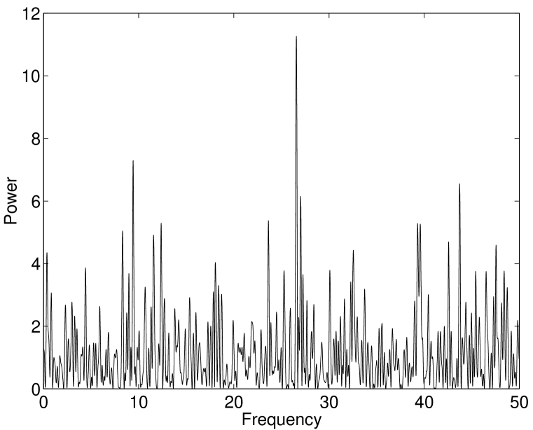
Figure 6: Power Spectrum of Super-Kamiokande 10-day data computed by the likelihood method.

We previously noted [15] that 9.42 y^-1 and 26.57 y^-1 sum to 35.99 y^-1, which is the sampling frequency, from which we inferred that one peak is spurious, being an alias of the other. Since the peak at 26.57 y^-1 had the bigger power, and since it falls in the band of twice the synodic rotation frequency, we assumed that the peak at 9.42 y^-1 was merely an alias. However, when the Super-Kamiokande data were subdivided into 5-day bins [18], the peak at 26.57 y^-1 disappeared, but the peak at 9.42 y^-1 remained. Hence it was clear that the peak at 26.57 y^-1 was an alias of the peak at 9.42 y^-1, not the other way around.

We analyzed the new Super-Kamiokande 5-day data using the likelihood procedure, taking account of the experimental statistical error estimates, the mean live time and the start and end time of each bin [38]. The resulting power spectrum is shown in Figure 7. The biggest peak, A, in the range 0–100 y^-1 is that at $9.43\pm 0.05$ y^-1, which now has the enhanced power $S=11.51$. In agreement with the analysis of the Super-Kamiokande group, we find that the peak at 26.57 y^-1 has disappeared. Hence 9.43 y^-1 is the primary peak, and the 26.57 y^-1 peak was merely an alias in the 10-day data. Since the 5-day binning is also very regular, the power spectrum of the timing now has a huge peak at 72.01 y^-1 (period 5.07 days), so an alias peak would be expected at $72.01-9.43=62.58$ y^-1, and we do indeed find a peak (not shown in Fig. 7) at $\nu=62.56\pm 0.08$ y^-1 with $S=5.36$. There are also notable peaks at $39.28\pm 0.05$ y^-1 ($S=8.91$), labeled C, and $43.72\pm 0.06$ y^-1 ($S=9.83$), labeled B in Fig. 7. The latter two peaks, plus that at 9.43 y^-1, are the three strongest peaks in the range 0–100 y^-1. Furthermore, the three peaks A, B, and C are all stronger in the 5-day dataset than in the 10-day dataset, as one would expect of real modulation, because of the difference in the sampling time.

Figure 7: Power Spectrum of Super-Kamiokande 5-day data computed by the likelihood method, taking account of measurement error, start time, and end time, of each bin.

6 Explanation for the Peak Frequencies

To understand these three peaks, it is helpful to seek guidance from measurements of the solar magnetic field. A power spectrum out to 120 y^-1 of the photospheric field at Sun-center during the Super-Kamiokande data-acquisition interval is shown in Figure 8. We see that the fundamental and second harmonic of the rotation frequency are virtually absent, but there is a remarkable sequence of higher harmonics. By forming the combined spectrum statistic [9] of the third through the seventh harmonics, we obtain the estimate $13.20\pm 0.14$ y^-1 for the synodic rotation frequency of the photospheric magnetic field, leading to the value $14.20\pm 0.14$ y^-1 for the sidereal rotation frequency.

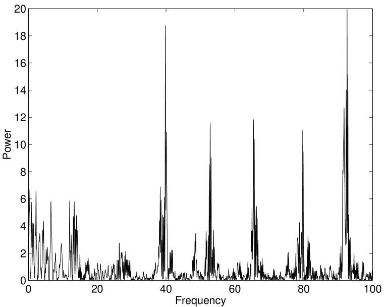
Figure 8: Power spectrum of the disk-center solar magnetic field for the interval of operation of Super-Kamiokande.

We see that peak C, at 39.28 y^-1, falls within the band of frequencies, $39.60\pm 0.42$ y^-1, of the third harmonic of the synodic rotation frequency of the magnetic field. We have applied the shuffle test [3, 39], randomly re-assigning flux and error measurements (kept together) to time bins. For this purpose, the shuffle test is more reliable than Monte Carlo simulations, since by using actual data there is no need to assume some form for the probability distribution function of the simulated data. In this way we find that only 5 of 1,000 simulations yield a power larger than 8.91 (the power of peak C) in this search band. It appears, therefore, that peak C may be attributed to the effect of the Sun’s internal inhomogeneous magnetic field that necessarily rotates with the ambient medium. To check this assumption, we have determined the frequency for which the neutrino and magnetic data show the strongest correlation by means of the joint spectrum statistic [9]. This frequency is found to be 39.56 y^-1. Figure 9 shows the cumulative Rayleigh powers derived from the neutrino and magnetic data for this frequency. We see that there is a remarkable correspondence, both powers growing from 1996 until 1998, then decreasing until about 2000.6 (solar maximum), after which both increase sharply, indicating again the influence of the solar cycle variations of magnetic structures in the convection zone.

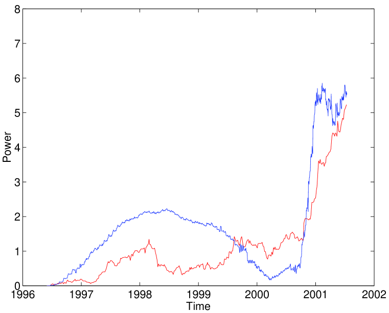
Figure 9: Cumulative contribution to the final Rayleigh power of disk-center magnetic field (blue) and 5-day Super-Kamiokande data (red) for frequency 39.56 y^-1. The steep rise begins near solar maximum (2000.6).

We now consider peak A at 9.43 y^-1 with power 11.51, and peak B at 43.72 y^-1 with power 9.83. We presented evidence above for r-mode oscillations [33] in the Homestake and GALLEX-GNO data that appear to be the origin of the well-known Rieger oscillation [31] and of similar “Rieger-type” oscillations [32] that have been discovered in recent years. We have therefore examined the possibility that peaks A and B may be related to such oscillations interpreted as r modes.

R-modes are retrograde waves that, in a uniform and uniformly rotating model Sun, have frequencies

$$\nu(\ell,m,{\rm syn})=m(\nu_{R}-1)-\frac{2m\nu_{R}}{\ell(\ell+1)}$$ (2)

as seen from Earth, where $\ell$ and $m$ are two of the usual spherical-harmonic indices, and $\nu_{R}$ is the sidereal rotation frequency (in cycles per year). If r-mode oscillations are to influence the solar neutrino flux, they must interfere with magnetic regions that co-rotate with the ambient medium. The interference frequencies will be given by

$$\nu=\left|m(\nu_{R}-1)-\frac{2m\nu_{R}}{\ell(\ell+1)}\pm m^{\prime}(\nu_{R}-1)\right|$$ (3)

where $m^{\prime}$, the azimuthal index for the magnetic structure, may be different from that of the r-mode. For $m^{\prime}=m$, equation (3) yields the frequency

$$\nu(\ell,m,{\rm rot})=\frac{2m\nu_{R}}{\ell(\ell+1)},$$ (4)

for the minus sign, and

$$\nu(\ell,m,{\rm alias})=2m(\nu_{R}-1)-\frac{2m\nu_{R}}{\ell(\ell+1)}$$ (5)

for the plus sign. The frequencies given by (4) are the well-known Rieger-type frequencies, which we showed in Sect. 2 were found in the Cl and Ga data. We may regard the frequencies given by (5) as aliases of these frequencies.

For $\ell=2$ and $m=2$ and for the range of values of $\nu_{R}$ inferred from the magnetic-field data, equation (4) leads us to expect oscillations in the band $9.47\pm 0.09$, and equation (5) leads us to expect oscillations in the band $43.33\pm 0.47$. We see that the peaks A and B fall within these bands. On applying the shuffle test, we find only 2 cases out of 10,000 in which a peak with power larger than 11.51 occurs in the band $9.47\pm 0.09$, and only 3 cases out of 1,000 that yield a power larger than 9.83 in the band $43.33\pm 0.47$. Figure 10 shows the cumulative Rayleigh powers at these two frequencies as a function of time. These two power components have a very similar trend in their time evolution, indicating that they both originate in the same internal oscillation, an r-mode with $\ell=2$, $m=2$. Note the contrast between Figs. 9 and 10, showing the different origins of the A and B peaks from that of C.

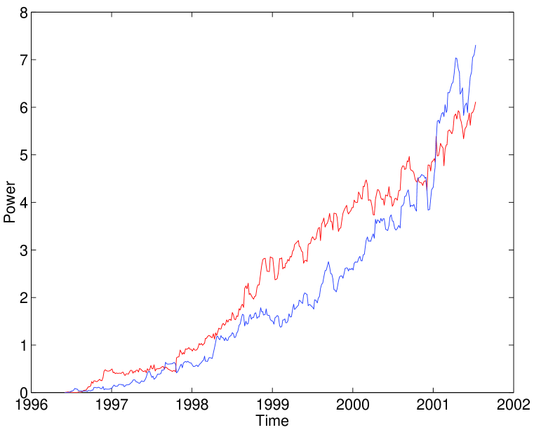
Figure 10: Cumulative contribution to the final Rayleigh powers of oscillations at 9.42 y^-1 (red) and 43.72 y^-1 (blue).

7 Discussion of the Frequency Peaks

In the previous Section we have shown that frequency peaks A (9.43 y^-1) and B (43.72 y^-1) are not only related to each other, but also that they can be quantitatively explained as r-mode oscillations when one determines the rotation rate of the solar magnetic field from observations. Frequency peak C (39.28 y^-1) was shown to be the same as the third harmonic of the magnetic field rotation rate, the only harmonic in the search band which was sufficiently prominent, since the fundamental and second harmonic were weak. Peak C illustrates the difficulty in predicting which frequency peaks will be important, since at the 2000.6 solar maximum the field broke up into structures which made third and seventh harmonics of the rotation rate especially strong, as shown in Fig. 8.

These same three peaks are seen in the analysis of the Super-Kamiokande group [18], but they claim them not to be statistically significant. In another paper [40] we have addressed this disagreement in detail, but some of the results will be summarized here. All comparisons are made standardizing on the 5-day data, a 0 to 50 y^-1 search band, and a Monte Carlo method to provide the statistical significance of the strongest peak. With the analysis method used by Super-Kamiokande, the Lomb-Scargle procedure with the mean live times, the leading peak has a power of 7.29 at frequency 43.73 y^-1. Since 32% of the simulations have power equal to or greater than 7.29, the result is clearly not statistically significant, in agreement with the conclusion of Yoo et al. [18]. If instead one uses a modified Lomb-Scargle analysis [37], employing again the mean live time but now taking into account the average statistical error of each data-point, the most significant peak becomes that at 9.43 y^-1 with a power of 9.56, which is significant at the 95% confidence level. This analysis still assumes that each data-point occurs at a unique time. By using the likelihood analysis one can take into account for each run the start time, end time, and mean live time, as well as the statistical errors. This increases the power of the 9.43 y^-1 peak to 11.67, which has a significance level of 99.3%. Clearly, by using this analysis method, we reach a different qualitative conclusion than do Yoo et al. [18].

As more experimental information is used, the significance of the flux modulation increases, as should be the case for a real signal. Yoo et al. [18] found from a sequence of Lomb-Scargle analyses using simulated data with a sinusoidally varying neutrino flux that, for periods of 20 days or more, they could not identify a signal if the depth of modulation is less than 10%. Since we find the depth of modulation at 9.43 y^-1 (period 38.73 days) is only 7%, we agree that they could not identify it reliably, whereas our more sensitive analysis method does.

8 Significance for Neutrino Physics

The evidence given above for neutrino flux variability in the Cl, Ga, and Super-Kamiokande data indicates that our current understanding of either the Sun or the neutrino model is inadequate. Changes in solar physics such as non-steady or non-spherically symmetric nuclear burning would be difficult to reconcile with the neutrino flux frequencies observed, or their apparent location in some cases in the solar convection zone. Association of these frequencies with the solar magnetic field rotation rates points very strongly to their cause involving the Resonant-Spin-Flavor-Precession (RSFP) process. This can occur, however, only subdominantly to the MSW effect. The use of RSFP would be simplest with the three known light active neutrinos, the mass differences of which force the process to take place in the solar core (from 0.05 $R_{\odot}$ at neutrino energy 3.35 MeV to 0.20 $R_{\odot}$ at 13 MeV [12]), with the MSW effect for each energy at a slightly larger radius. There are several disagreements between this solution and the results of our analyses. First, flux modulations show in all cases but one frequencies corresponding to solar rotation rates in the convection zone above the tachocline ($\sim 0.7R_{\odot}$). See Fig. 1, for instance. Second, the depth of modulation in this model is too small. In the Super-Kamiokande energy region the predicted [12] modulation is $\sim 2$–3%, but we find about 7%. Third, the depth of modulation is predicted [12] to increase with neutrino energy, being 0.77% at 2.50 MeV and 1.03% at 3.35 MeV, whereas we find large effects at low energy; see Fig. 4, for example.

The next simplest model, which we introduced reluctantly some time ago, now seems forced upon us. Already the large transition magnetic moment required for RSFP necessitates new physics, so one hopes that the need for a sterile neutrino arises from the same new physics. The sterile neutrino is required for a fit to the data, for example to provide $\Delta m^{2}\sim 10^{-8}$ eV² needed to have RSFP in the convection zone. Such a mass difference was essential even to fit the time-averaged solar data when RSFP alone was used [22, 23]. For the same reason that RSFP gave such a good fit to the data (i.e., the energy dependence of the neutrino survival probability), invoking it subdominantly in this sterile neutrino model solves [11] two current problems with the fits that occur when MSW alone is used. In addition to these positive qualities, the usual negative ones are avoided. The lack of solar antineutrinos places no limitation on RSFP because of the sterile final state. Constraints from unitarity using atmospheric and solar neutrino data are avoided, since the sterile neutrino does not mix with active ones. For the same reason nucleosynthesis considerations provide no limits. There is also sufficient uncertainty in the fraction of solar neutrinos oscillating into active neutrinos in the ⁸B energy region to allow for the needed quantity of sterile final states [41]. Finally, it has been shown [11] that this model can accommodate the depths of modulation required. For a reasonable magnetic field shape (profile 2 in [11]), the maximum modulation depths are found to be about 15% in the Super-Kamiokande energy region, 17% for Cl, and 40% for Ga. Thus in every respect investigated, the model of a sterile neutrino coupled to the electron neutrino via only a transition magnetic moment satisfies the empirical information.

9 Predictions and Conclusions

The analysis of Super-Kamiokande data, when combined with the results of analyses of Cl and Ga data, yields a variety of evidence for variability of the solar neutrino flux. It should be stressed that this evidence can in principle all be understood in terms of known fluid-dynamic and solar-dynamic processes in the standard solar model. In particular, the frequency peaks in the Super-Kamiokande data are all explained. These same peaks are seen in the analysis by the Super-Kamiokande collaboration, but their less sensitive method of analysis makes these peaks appear insignificant, whereas our method, that uses more of the experimental information, can reveal these small modulations [40].

Although it is normal—perhaps inevitable—in exploratory research that one examines the results of an analysis and then seeks to interpret the results in known terms, this is a process that one would like to avoid. In mature research, one would begin with a prediction, and then look to see if that prediction is borne out in a new study.

This procedure will be difficult to implement within the context of solar neutrino modulation, for several reasons: we have inadequate information concerning the flows and magnetic fields deep in the solar interior, we must hypothesize about the neutrino physics involved, and we have inadequate understanding of the way in which dynamical processes near the tachocline lead to observable consequences at the photosphere and above. Although helioseismology has greatly improved our knowledge of the solar interior in recent years, solar physics is not yet at the stage that we can safely infer, from observational data, the flows and magnetic structures which occur deep in the solar interior.

However, one may at this stage consider two sources of periodic modulation that are well established, rotational effects and Rieger-type oscillations [31, 32], and attempt to identify search bands associated with these dynamical processes. We may expect to find modulation corresponding to the synodic rotation frequency in the solar equatorial plane ($13.20\pm 0.14$ yr^-1) or a low harmonic of this frequency, such as the second ($26.40\pm 0.28$ yr^-1) or third ($29.60\pm 0.42$ yr^-1). The power resulting from modulation at a given amplitude decreases as $(2\pi\nu D)^{-2}$ where $D$ is the average length of each time bin [38], so that high harmonics will be difficult to detect. Aliases of the higher harmonics would be correspondingly suppressed. Concerning the Rieger-type oscillations, we propose that they may be attributed r-mode oscillations, specifically the $\ell=3$, $m=1$ mode ($2.20\pm 0.02$ yr^-1), the $\ell=3$, $m=3$ mode ($6.50\pm 0.07$ yr^-1), and either the $\ell=3$, $m=2$ mode or the $\ell=2$, $m=1$ mode, which have the same frequency ($4.40\pm 0.05$ yr^-1). Hence it would be reasonable to search for these modes and also the $\ell=2$, $m=2$ mode ($9.47\pm 0.09$ yr^-1).

We apply this simple approach to the Super-Kamiokande power spectrum. Concerning the rotational frequency bands, we found a signal with power $S=8.91$ in the third band. For the specified search band, we found from the shuffle test that the probability of obtaining this strong a peak by chance is 0.005. The probability of obtaining this result by chance in three “trials” (for the three rotational bands being considered) is 0.015. Concerning the four 4-mode bands being considered, we find a peak in one of them ($\ell=2$, $m=2$) with power $S=11.51$. We find from the shuffle test that the probability of obtaining this strong peak by chance in the relevant search band is 0.003. The probability of obtaining this result by chance in four “trials” for the four 4-mode bands being considered is 0.012.

We now need to estimate the probability of obtaining both results in the same dataset. From the relation $P=e^{-S}$, we find that p-values of 0.015 and 0.012 convert to power values of 4.20 and 4.42, respectively. The corresponding combined power statistic [9]

$$G=Z-\ln(1+Z),$$ (6)

where $Z$ is the sum of the powers (i.e., 8.62), has the value 6.36. Hence there is a probability of 0.0017 of obtaining these two peaks in these seven search bands by chance.

This small probability does not utilize all the information in Fig. 8, which shows why only the one harmonic found in the neutrino data could be observed, provided the photospheric magnetic field represents that in the solar interior. There is no similar guidance in the r-mode case, since too little is known about the complex solar interior “weather” to predict which of the peaks should be observable. For a different neutrino energy and solar cycle, the other three r-modes were observed in the Cl and Ga experiments, as described toward the end of Sec. 2. Concerning the “alias” r-mode frequencies given by Eq. 5, we should comment that, to the best of our knowledge, these have not previously been identified in solar data, so it will be interesting to see if they show up in subsequent neutrino data.

More precise specification of expected frequencies does not appear possible at this time. That is why the power spectrum analysis of the SNO data, expected shortly, is so important. The SNO and Super-Kamiokande experiments had some overlap in time of operation and observed a similar neutrino energy range. If one-day bins are used, the alias peak at 62.56 y^-1 should not be seen, but the r-mode frequencies of Fig. 10 at 9.43 y^-1 and 43.72 y^-1 should be. In data taken in the solar cycle after 2000.6, the 39.3 y^-1 frequency of Fig. 9 should be present, and with shorter sampling time, some of the higher harmonics of the magnetic field rotation may also be observed.

Other types of tests exist of the RSFP framework, which appears to explain so well the current information on solar neutrino flux variations. First, experiments are being instrumented to measure electron neutrino magnetic moments as low as $\sim 10^{-12}\mu_{B}$, which is in the range of interest. Second, future measurements of the ⁷Be neutrino flux are likely to give a much lower value of the time-averaged flux than predicted by the LMA solution.

The potential explanation for the cause of solar neutrino flux variability makes proof of the effect all the more important. In view of the results of the KamLAND experiment, a subdominant RSFP process appears to be required, and this necessitates coupling the electron neutrino to a sterile neutrino via only a large transition magnetic moment. Such new physics, which appears compatible with all known limitations and observations, should have many significant consequences.

10 Acknowledgments

We are indebted to G.M. Fuller, J.D. Scargle, G. Walther, M.S. Wheatland, and S.J. Yellin for assistance and helpful discussions. D.O.C. has been supported in part by a grant from the Department of Energy No. DE-FG03-91ER40618, and P.A.S. is supported by grant No. AST-0097128 from the National Science Foundation.

Appendix A Appendix: Brief Explanation of the Likelihood Calculation

The log-likelihood that the data $x_{r}$ may be fit by a given functional form $X_{r}$ is given [38] by

$$L=-\frac{1}{2}\sum^{R}_{r=1}\frac{(x_{r}-X_{r})^{2}}{\sigma^{2}_{r}},$$

apart from a constant term, where $r=1,\ldots,R$ enumerates the data bins. We adopt

$$x_{r}=\frac{g_{r}}{{\rm mean}(g_{r})}-1,$$

where $g_{r}$ are the flux measurements, and scale the error estimates accordingly. We adopt the functional form

$$X_{r}=\frac{1}{D_{r}}\int^{t_{er}}_{t_{sr}}dt(Ae^{i2\pi\nu t}+A^{*}e^{-i2\pi\nu t}),$$

where $D_{r}$ is the duration of each bin. Then, for each frequency, we adjust the amplitude A to maximize the likelihood [3].

What is significant is not the actual log-likelihood as computed from (1), but the increase in the log-likelihood over the value that corresponds to a constant flux, which is given (apart from the same constant term) by

$$L_{0}=-\frac{1}{2}\sum^{R}_{r=1}\frac{x^{2}_{r}}{\sigma^{2}_{r}}.$$

Hence the relative log-likelihood, which is equivalent to the power spectrum, is given by

$$S=L-L_{0},$$

i.e., by

$$S=\frac{1}{2}\sum^{R}_{r=1}\frac{x^{2}_{r}}{\sigma^{2}_{r}}-\frac{1}{2}\sum^{R}_{r=1}\frac{(x_{r}-X_{r})^{2}}{\sigma^{2}_{r}}.$$

Application of the formalism above to one frequency in the Super-Kamiokande data shows the magnitude of the flux modulation. For $\nu=9.43$, and for zero time chosen arbitrarily to be the date 1970.00, we find that $A=0.0192-0.0291i$. This corresponds to a depth of modulation of the neutrino flux of 7%.

References

- [1] K. Eguchi et al., Phys. Rev. Lett. 90, 021802 (2003).
- [2] C.-S. Lim and W.J. Marciano, Phys. Rev. D 37, 1368 (1988); E.Kh. Akhmedov, Sov. J. Nucl. Phys. 48, 382 (1988) and Phys. Lett. B213, 64 (1988).
- [3] P.A. Sturrock, G. Walther and M.S. Wheatland, Astrophys. J. 491, 409 (1997).
- [4] P.A. Sturrock, G. Walther and M.S. Wheatland, Astrophys. J. 507, 978 (1998).
- [5] P.A. Sturrock, J.D. Scargle, G. Walther and M.S. Wheatland, Astrophys. J. 523, L177 (1999).
- [6] P.A. Sturrock and J.D. Scargle, Astrophys. J. 550, L101 (2000).
- [7] P.A. Sturrock and M.A. Weber, Astrophys. J. 565, 1366 (2002).
- [8] P.A. Sturrock and M.A. Weber, “Multi-Wavelength Observations of Coronal Structure and Dynamics—Yohkoh 10th Anniversary Meeting” (COSPAR Colloquia Series, P.C.H. Martens and D. Cauffman, eds., 2002), p. 323.
- [9] P.A. Sturrock, astro-ph/0304148; P.A. Sturrock and M.S. Wheatland, astro-ph/0307353; P.A. Sturrock, J.D. Scargle, G. Walther and M.S. Wheatland, Solar Physics (in press, 2005).
- [10] P.A. Sturrock, hep-ph/0304106.
- [11] B.C. Chauhan and J. Pulido, JHEP 0406, 008 (2004). The neutrino model used was suggested by one of us (D.O.C.) in a much earlier version of this present paper, but delayed publication now enables us to utilize their excellent results.
- [12] A.B. Balantekin and C. Volpe, hep-ph/0411148.
- [13] S. Fukuda et al., Phys. Rev. Lett. 86, 5651 (2001).
- [14] M.B. Smy, hep-ex/0206016 and http://www-sk.icrr.u-tokyo.ac.jp/sk/lowe/index.html
- [15] P.A. Sturrock and D.O. Caldwell, Bull. Am. Astron. Soc. 34, 1314 (2002); P.A. Sturrock, Astrophys. J. 594, 1102 (2004). D.O. Caldwell and P.A. Sturrock, hep-ph/0305303.
- [16] A. Milsztajn, hep-ph/0301252.
- [17] M. Nakahata, http://www-sk.icrr.u-tokyo.ac.jp/sk/lowe/frequencyanalysis/ index.html.
- [18] J. Yoo et al., Phys. Rev. D 68, 092002 (2003).
- [19] L. Wolfenstein, Phys. Rev. D 17, 2369 (1978); Phys. Rev. D 20, 2634 (1979); S.P. Mikheyev and A.Yu. Smirnov, Sov. J. Nucl. Phys. 42, 913 (1985); Nuovo Cimento 9C, 17 (1986).
- [20] P.C. de Holanda and A.Yu. Smirnov, Phys. Rev. D 69, 113002 (2004).
- [21] B.T. Cleveland et al., Astrophys. J. 496, 505 (1998).
- [22] M.M. Guzzo and H. Nunokawa, Astropart. Phys. 12, 87 (1999); J. Pulido and E.Kh. Akhmedov, Astropart. Phys. 13, 227 (2000); E.Kh. Akhmedov and J. Pulido, Phys. Lett. B485, 178 (2000); O.G. Miranda, C. Peña-Garay, T.I. Rashba, V.B. Semikoz and J.W.F. Valle, Nucl. Phys. B595, 360 (2001) and Phys. Lett. B521, 299 (2001); J. Pulido, Astropart. Phys. 18, 173 (2002).
- [23] B.C. Chauhan and J. Pulido, Phys. Rev. D 66, 053006 (2002) includes the SNO data in the fits.
- [24] Q.R. Ahmad et al., Phys. Rev. Lett. 89, 011301 and 011302 (2002).
- [25] A. Aguilar et al., Phys. Rev. D 64, 112007 (2001) and earlier references therein.
- [26] W. Hampel et al., Phys. Lett. B447, 127 (1999); M. Altmann et al., Phys. Lett. B490, 16 (2000).
- [27] J. Schou et al., Astrophys. J. 505, 390 (1998).
- [28] S. Tsuneta et al., Solar Phys. 136, 37 (1991).
- [29] E. Antonucci et al., Astrophys. J. 360, 296 (1998).
- [30] T. Bai, Bull. Am. Astron. Soc. 34, 953 (2002).
- [31] E. Rieger et al., Nature 312, 623 (1984).
- [32] T. Bai, Astrophys. J. 388, L69 (1992); Solar Phys. 150, 385 (1994); J.N. Kile, and E.W. Cliver, Astrophys. J. 370, 442 (1991).
- [33] J. Papaloizou, and J.E. Pringle, Mon. Not. R. Astro. Soc. 182, 423 (1978); J. Provost, G. Berthomieu, and A. Rocca, Astron. Astrophys. 94, 126 (1981); H. Saio, Astrophys. J. 256, 717 (1982).
- [34] A. Friedland and A. Gruzinov, Astropart. Phys. 19, 575 (2003).
- [35] L. Pandola, Astropart. Phys. 22, 219 (2004).
- [36] P.A. Sturrock and D.O. Caldwell, hep-ph/0409064.
- [37] N. Lomb, Astrophys. Space Sci. 39, 447 (1996); further developed by J.D. Scargle, Astrophys. J. 263, 835 (1982); Astrophys. J. 343, 874 (1989).
- [38] P.A. Sturrock, Astrophys. J. 594, 1102 (2003); ibid. 605, 568 (2004).
- [39] J.N. Bahcall and W.H. Press, Astrophys. J. 370, 730 (1991).
- [40] P.A. Sturrock, D.O. Caldwell, J.D. Scargle, and M.S. Wheatland, hep-ph/0501205.
- [41] A.B. Balantekin, V. Barger, D. Marfatia, S. Pakvasa, and H. Yüksel, Phys. Lett. B613, 61 (2005); B.C. Chauhan and J. Pulido, JHEP 042, 040 (2004).