Charged Kaon $K\to 3\pi$ CP Violating Asymmetries
at NLO in CHPT

Abstract:

We give the first full next-to-leading order analytical results in Chiral Perturbation Theory for the charged Kaon $K\to 3\pi$ slope $g$ and decay rates CP-violating asymmetries. We have included the dominant Final State Interactions at NLO analytically and discussed the importance of the unknown counterterms. We find that the uncertainty due to them is reasonable just for $\Delta g_{C}$, i.e. the asymmetry in the $K^{+}\to\pi^{+}\pi^{+}\pi^{-}$ slope $g$, we get $\Delta g_{C}=-(2.4\pm 1.2)\times 10^{-5}$. The rest of the asymmetries are very sensitive to the unknown counterterms, in particular, the decay rate asymmetries can change even sign. One can use this large sentivity to get valuable information on those counterterms and on $\mbox{Im }G_{8}$ coupling –very important for the CP-violating parameter $\varepsilon^{\prime}_{K}$– from the eventual measurement of these asymmetries. We also provide the one-loop ${\cal O}(e^{2}p^{2})$ electroweak octet contributions for the neutral and charged Kaon $K\to 3\pi$ decays.

1 Introduction

The decay of a Kaon into three pions has a long history. The first calculations were done using current algebra methods or tree level Lagrangians, see [1] and references therein. Then using Chiral Perturbation Theory (CHPT) [2, 3] at tree level in [4]. Some introductory lectures on CHPT can be found in [5] and recent reviews in [6].

The one-loop calculation was done in [7, 8] and used in [9], unfortunately the analytical full results were not available. Recently, there has appeared the first full published result in [10].

CP-violating observables in $K\to 3\pi$ decays have also attracted a lot of work since long time ago [11, 12, 13, 14, 15, 16, 17, 18, 19, 20, 21, 22] and references therein.

At next-to-leading order (NLO) there were no exact results available in CHPT so that the results presented in [16, 17, 18, 19] about the NLO corrections were based in assumptions about the behavior of those corrections and/or using model depending results in [16]. In [20, 21] there are partial results at NLO within the linear $\sigma$-model.

Recently, two experiments, namely, NA48 at CERN and KLOE at Frascati, have announced the possibility of measuring the asymmetry $\Delta g_{C}$ and $\Delta g_{N}$ with a sensitivity of the order of $10^{-4}$, i.e., two orders of magnitude better than at present [23], see for instance [24] and [25]. It is therefore mandatory to have these predictions at NLO in CHPT. The goal of this paper is to make such predictions.

In particular, we have explicitly checked the one-loop results of [10], we also provide the complete one-loop calculation for the electroweak octet contribution up to ${\cal O}(e^{2}p^{2})$ in CHPT for all the decays $K\rightarrow 3\pi$ and finally, we estimate the dominant FSI for the charged Kaon $K\rightarrow 3\pi$ decays. We use all this to make the first full NLO in CHPT predictions for the charged Kaon $K\to 3\pi$ slope $g$ and decay rates CP-violating asymmetries. We also present analytical results for all of our predictions.

Notation and definitions of the asymmetries are in Section 2. In Section 3 we collect the inputs that we use for the weak counterterms in the leading and next-to-leading order weak chiral Lagrangians. In Section 4 we give the CHPT predictions at leading- and next-to-leading order for the decay rates and the slopes $g$, $h$ and $k$. We discuss the results for the CP-violating asymmetries at leading order first in Section 5 and we discuss them at NLO in Section 6. Finally, we give the conclusions and make comparison with earlier work in Section 7. In Appendix A, the $\Delta S=1$ CHPT Lagrangian used at NLO can be found. In Appendix B we give the notation we use for the $K\to 3\pi$ amplitudes and the new results at order $e^{2}p^{2}$. In Appendix C we give the analytic formulas needed for the slope $g$ and the asymmetries $\Delta g$ at LO and NLO and in Appendix D the relevant quantities to calculate the decay rates $\Gamma$ and the CP-violating asymmetries in the decay rates $\Delta\Gamma$ also at LO and NLO. In Appendix E we give the analytical results for the dominant –two-bubble– FSI contribution to the decays of charged Kaons and to the CP-violating asymmetries at NLO order, i.e. order $p^{6}$.

2 Notation and Definitions

The lowest order SU(3) $\times$ SU(3) chiral Lagrangian describing $|\Delta S|=1$ transitions is

$${\cal L}^{(2)}_{|\Delta S|=1} = C\,F_{0}^{6}\,e^{2}\,G_{E}\,\mbox{tr}\left(\Delta_{32}u^{\dagger}Qu\right)+CF_{0}^{4}\left[G_{8}\,\mbox{tr}\left(\Delta_{32}u_{\mu}u^{\mu}\right)+G_{8}^{\prime}\mbox{tr}\left(\Delta_{32}\chi_{+}\right)\right.$$ (1)

$$+ \left.G_{27}\,t^{ij,kl}\,\mbox{tr}\left(\Delta_{ij}u_{\mu}\right)\,\mbox{tr}\left(\Delta_{kl}u^{\mu}\right)\right]+{\rm h.c.}$$

with

$$C=-\frac{3}{5}\frac{G_{F}}{\sqrt{2}}V_{ud}{V^{*}_{us}}\simeq-1.07\times 10^{-6}\,{\rm GeV}^{-2}\,.$$ (2)

The correspondence with the couplings $c_{2}$ and $c_{3}$ of [7, 8] is

$$c_{2}=CF_{0}^{4}\,G_{8};$$

$$c_{3}=-\frac{\displaystyle 1}{\displaystyle 6}CF_{0}^{4}\,G_{27}\,.$$ (3)

$F_{0}$ is the chiral limit value of the pion decay constant $f_{\pi}=(92.4\pm 0.4)$ MeV,

$$u_{\mu}\equiv iu^{\dagger}(D_{\mu}U)u^{\dagger}=u_{\mu}^{\dagger}\;,$$

$$\Delta_{ij}=u\lambda_{ij}u^{\dagger}\;(\lambda_{ij})_{ab}\equiv\delta_{ia}\delta_{jb}\;,$$

$$\chi_{+(-)}=u^{\dagger}\chi u^{\dagger}+(-)u\chi^{\dagger}u$$ (4)

$\chi=\mbox{diag}(m_{u},m_{d},m_{s})$ a 3 $\times$ 3 matrix collecting the light quark masses, $U\equiv u^{2}=\exp{(i\sqrt{2}\Phi/F_{0})}$ is the exponential representation incorporating the octet of light pseudo-scalar mesons in the SU(3) matrix $\Phi$;

$$\Phi\equiv\left(\begin{array}[]{ccc}\frac{\displaystyle\pi^{0}}{\displaystyle\sqrt{2}}+\frac{\displaystyle\eta_{8}}{\displaystyle\sqrt{6}}&\pi^{+}&K^{+}\\ \pi^{-}&-\frac{\displaystyle\pi^{0}}{\displaystyle\sqrt{2}}+\frac{\displaystyle\eta_{8}}{\displaystyle\sqrt{6}}&K^{0}\\ K^{-}&\bar{K^{0}}&-2\frac{\displaystyle\eta_{8}}{\displaystyle\sqrt{6}}\end{array}\right)\,.$$ (6)

The non-zero components of the SU(3) $\times$ SU(3) tensor $t^{ij,kl}$ are

$$t^{21,13}=t^{13,21}=\frac{1}{3}\,;\, t^{22,23}=t^{23,22}=-\frac{\displaystyle 1}{\displaystyle 6}\,;$$

$$t^{23,33}=t^{33,23}=-\frac{1}{6}\,;\, t^{23,11}=t^{11,23}=\frac{\displaystyle 1}{\displaystyle 3}\,;$$ (7)

and $Q=\mbox{diag}(2/3,-1/3,-1/3)$ is a 3 $\times$ 3 matrix which collects the electric charge of the three light quark flavors.

We calculate the amplitudes

$$K_{2}(k) \to \pi^{0}(p_{1})\pi^{0}(p_{2})\pi^{0}(p_{3})\,,\quad[A^{2}_{000}]\,,$$

$$K_{2}(k) \to \pi^{+}(p_{1})\pi^{-}(p_{2})\pi^{0}(p_{3})\,,\quad[A^{2}_{+-0}]\,,$$

$$K_{1}(k) \to \pi^{+}(p_{1})\pi^{-}(p_{2})\pi^{0}(p_{3})\,,\quad[A^{1}_{+-0}]\,,$$

$$K^{+}(k) \to \pi^{0}(p_{1})\pi^{0}(p_{2})\pi^{+}(p_{3})\,,\quad[A_{00+}]\,,$$

$$K^{+}(k) \to \pi^{+}(p_{1})\pi^{+}(p_{2})\pi^{-}(p_{3})\,,\quad[A_{++-}]\,,$$ (8)

as well as their CP-conjugated decays at NLO (i.e. order $p^{4}$ in this case) in the chiral expansion and in the isospin symmetry limit $m_{u}=m_{d}$. We have also calculated the contribution of the ${\cal O}(e^{2}p^{2})$ electroweak octet counterterms. In (2) we have indicated the four momentum carried by each particle and the symbol we will use for the amplitude. The states $K_{1}$ and $K_{2}$ are defined as

$$K_{1(2)}\,=\,\frac{K^{0}-(+)\overline{K^{0}}}{\sqrt{2}}\,.$$ (9)

For the explicit form of the Lagrangian we have used, see Appendix A. Our results for the octet and 27-plet terms fully agree with the results found in [10] so that we do not write them again. The electroweak contributions to $K\to 3\pi$ decays of order $e^{2}p^{0}$ and $e^{2}p^{2}$ can be found in Subsection B.1 in Appendix B.

In this paper we discuss CP-violating asymmetries in the decay of the charged Kaon into three pions; namely, asymmetries in the slope $g$ defined as

$$\frac{\left|A_{K^{+}\to 3\pi}(s_{1},s_{2},s_{3})\right|^{2}}{\left|A_{K^{+}\to 3\pi}(s_{0},s_{0},s_{0})\right|^{2}}=1+g\,y+h\,y^{2}+k\,x^{2}+{\cal O}(yx^{2},y^{3})\,$$ (10)

and some asymmetries in the integrated $K^{+}\to 3\pi$ decay rates. Above, we used the Dalitz variables

$$x\equiv\frac{s_{1}-s_{2}}{m_{\pi^{+}}^{2}} \hskip 14.22636pt{\rm and}\hskip 14.22636pt y\equiv\frac{s_{3}-s_{0}}{m_{\pi^{+}}^{2}}\,$$ (11)

with $s_{i}\equiv(k-p_{i})^{2}$, $3s_{0}\equiv m_{K}^{2}+m_{\pi^{(1)}}^{2}+m_{\pi^{(2)}}^{2}+m_{\pi^{(3)}}^{2}$.

The CP-violating asymmetries in the slope $g$ are defined as

$$\Delta g_{C}\equiv\frac{g[K^{+}\to\pi^{+}\pi^{+}\pi^{-}]-g[K^{-}\to\pi^{-}\pi^{-}\pi^{+}]}{g[K^{+}\to\pi^{+}\pi^{+}\pi^{-}]+g[K^{-}\to\pi^{-}\pi^{-}\pi^{+}]}$$

$${\rm and}\hskip 14.22636pt\Delta g_{N}\equiv\frac{g[K^{+}\to\pi^{0}\pi^{0}\pi^{+}]-g[K^{-}\to\pi^{0}\pi^{0}\pi^{-}]}{g[K^{+}\to\pi^{0}\pi^{0}\pi^{+}]+g[K^{-}\to\pi^{0}\pi^{0}\pi^{-}]}\,.$$ (12)

A first update at LO of these asymmetries was already presented in [26].

The CP-violating asymmetries in the decay rates are defined as

$$\Delta\Gamma_{C}\equiv\frac{\Gamma[K^{+}\to\pi^{+}\pi^{+}\pi^{-}]-\Gamma[K^{-}\to\pi^{-}\pi^{-}\pi^{+}]}{\Gamma[K^{+}\to\pi^{+}\pi^{+}\pi^{-}]+\Gamma[K^{-}\to\pi^{-}\pi^{-}\pi^{+}]}$$

$${\rm and}\hskip 14.22636pt\Delta\Gamma_{N}\equiv\frac{\Gamma[K^{+}\to\pi^{0}\pi^{0}\pi^{+}]-\Gamma[K^{-}\to\pi^{0}\pi^{0}\pi^{-}]}{\Gamma[K^{+}\to\pi^{0}\pi^{0}\pi^{+}]+\Gamma[K^{-}\to\pi^{0}\pi^{0}\pi^{-}]}\,.$$ (13)

In particular, we also want to check the statement that with appropriate cuts one can get one order of magnitude enhancement in $\Delta\Gamma_{C}$ and $\Delta\Gamma_{N}$ asymmetries [13].

3 Numerical Inputs for the Weak Chiral Counterterms

Here we collect the values of the weak chiral counterterms that we use in this work.

3.1 Counterterms of the LO Weak Chiral Lagrangian

In [10], a fit to all available $K\to\pi\pi$ amplitudes at NLO in CHPT [27] and $K\to 3\pi$ amplitudes and slopes in the $K\to 3\pi$ amplitudes at NLO in CHPT was done. The result found there for the ratio of the isospin definite [0 and 2] $K\to\pi\pi$ amplitudes to all orders in CHPT was

$$\frac{A_{0}[K\to\pi\pi]}{A_{2}[K\to\pi\pi]}=21.8\,;$$ (14)

giving the infamous $\Delta I=1/2$ rule for Kaons and

$$\left[\frac{A_{0}[K\to\pi\pi]}{A_{2}[K\to\pi\pi]}\right]^{(2)}=17.8\,,$$ (15)

to lowest CHPT order $p^{2}$. I.e., Final State Interactions and the rest of higher order corrections are responsible for 22% of the $\Delta I=1/2$ enhancement rule. Yet most of this enhancement appears at lowest CHPT order! The last result is equivalent [using $F_{0}=87.7$ MeV] to

$$\mbox{Re }G_{8}=6.8\pm 0.6 \hskip 14.22636pt{\rm and}\hskip 14.22636pt G_{27}=0.48\pm 0.06\,.$$ (16)

In this normalization, $\mbox{Re }G_{8}=G_{27}=1$ at large $N_{c}$. No information can be obtained for $\mbox{Re }(e^{2}G_{E})$ due to its tiny contribution to CP-conserving amplitudes.

CP-conserving observables are fixed by physical meson masses, the pion decay coupling in the chiral limit $F_{0}$ and the real part of the counterterms. To predict CP-violating asymmetries we also need the values of the imaginary part of these couplings. Let us see what we know about them. At large $N_{c}$, all the contributions to $\mbox{Im }G_{8}$ and $\mbox{Im }(e^{2}G_{E})$ are factorizable and the scheme dependences are not under control. The unfactorizable topologies are not included at this order and they bring in unrelated dynamics with its new scale and scheme dependence, so that one cannot give an uncertainty to the large $N_{c}$ result for $\mbox{Im }G_{8}$ and $\mbox{Im }(e^{2}G_{E})$. We get

$$\mbox{Im }G_{8}\Big{|}_{N_{c}}\!\!\! = \!\!\!\,1.9\,\mbox{Im }\tau\,,$$

$$\mbox{Im }(e^{2}G_{E})\Big{|}_{N_{c}}\!\!\! = \!\!\!\,-2.9\,\mbox{Im }\tau\,.$$ (17)

In the Standard Model [28]

$$\mbox{Im }\tau\equiv-\mbox{Im }\left(\frac{V_{td}V^{*}_{ts}}{V_{ud}V^{*}_{us}}\right)\simeq-(6.05\pm 0.50)\times 10^{-4}\,,$$ (18)

and we used [29]

$$\langle 0|\overline{q}q|0\rangle_{\overline{\rm MS}}(2{\rm GeV})=-(0.018\pm 0.004)\,{\rm GeV}^{3}$$ (19)

which agrees with the most recent sum rule determinations of this condensate and of light quark masses –see [30] for instance– and the lattice light quark masses world average [31].

There have been recently advances on going beyond the leading order in $1/N_{c}$ in both couplings, $\mbox{Im }G_{8}$ and $\mbox{Im }(e^{2}G_{E})$.

In [32, 33, 34], there are recent model independent calculations of $\mbox{Im }(e^{2}G_{E})$. The results there are valid to all orders in $1/N_{c}$ and NLO in $\alpha_{S}$. They are obtained using the hadronic tau data collected by ALEPH [35] and OPAL [36] at LEP. The agreement is quite good between them and their results can be summarized in

$$\mbox{Im }(e^{2}G_{E})=-(4.0\pm 0.9)\,\mbox{Im }\tau\,,$$ (20)

where the central value is an average and the error is the smallest one. In [37] it was used a Minimal Hadronic Approximation to large $N_{c}$ to calculate $\mbox{Im }(e^{2}G_{E})$, they got

$$\mbox{Im }(e^{2}G_{E})=-(6.7\pm 2.0)\,\mbox{Im }\tau\,,$$ (21)

which is also in agreement though somewhat larger. There are also lattice results for $\mbox{Im }(e^{2}G_{E})$ both using domain-wall fermions [38] and Wilson fermions [39]. All of them made the chiral limit extrapolations, their results are in agreement between themselves and their average gives

$$\mbox{Im }(e^{2}G_{E})=-(3.2\pm 0.3)\,\mbox{Im }\tau\,.$$ (22)

There are also results on $\mbox{Im }G_{8}$ at NLO in $1/N_{c}$. In [40], the authors made a calculation using a hadronic model which reproduced the $\Delta I=1/2$ rule for Kaons through a very large $Q_{2}$ penguin-like contribution –see [41] for details. The results obtained there are

$$\mbox{Re }G_{8}=6.0\pm 1.7,\,\,\, {\rm and} G_{27}=0.35\pm 0.15\,,$$ (23)

in very good agreement with the experimental results in (16).

The result found in [40] is

$$\mbox{Im }G_{8}=(4.4\pm 2.2)\,\mbox{Im }\tau$$ (24)

at NLO in $1/N_{c}$. The hadronic model used there had however some drawbacks [42] which have been eliminated in the ladder resummation hadronic model in [43]. The work in [40, 41] will be eventually updated using this hadronic model.

In [40] there was also a determination of $\mbox{Re }(e^{2}G_{E})$ though very uncertain. However, since the contribution of $\mbox{Re }(e^{2}G_{E})$ is very small in all the quantities we calculate, we take the value from [40] with 100% uncertainty and add its contribution to the error of those quantities.

Very recently, using a Minimal Hadronic Approximation to large $N_{c}$, the authors of [44] found qualitatively similar results to those in [40]. I.e. enhancement toward the explanation of the $\Delta I=1/2$ rule through $Q_{2}$ penguin-like diagrams and a matrix element of the gluonic penguin $Q_{6}$ around three times the factorisable contribution. The same type of enhancement though less moderate was already found in [45].

3.2 Counterterms of the NLO Weak Chiral Lagrangian

To describe $K\to 3\pi$ at NLO, in addition to $\mbox{Re }G_{8}$, $G_{27}$, $\mbox{Re }(e^{2}G_{E})$, $\mbox{Im }G_{8}$ and $\mbox{Im }(e^{2}G_{E})$, we also need several other ingredients. Namely, for the real part we need the chiral logs and the counterterms. The relevant counterterm combinations were called $\widetilde{K}_{i}$ in [10]. The chiral logs are fully analytically known [10] –we have confirmed them in the present work. The real part of the counterterms, $\mbox{Re }\widetilde{K}_{i}$, can be obtained from the fit of the $K\to 3\pi$ CP-conserving decays to data done in [10]. The relation of the $\widetilde{K}_{i}$ counterterms and those defined in Appendix A, and the values used for them are in Table 1 and Table 2 respectively.

$\widetilde{K}_{1}$	$\mbox{Re }(G_{8})(N_{5}^{r}-2N_{7}^{r}+2N_{8}^{r}+N_{9}^{r})+G_{27}\left(-\frac{1}{2}D_{6}^{r}\right)$
$\widetilde{K}_{2}$	$\mbox{Re }(G_{8})(N_{1}^{r}+N_{2}^{r})+G_{27}\left(\frac{1}{3}D_{26}^{r}-\frac{4}{3}D_{28}^{r}\right)$
$\widetilde{K}_{3}$	$\mbox{Re }(G_{8})(N_{3}^{r})+G_{27}\left(\frac{2}{3}D_{27}^{r}+\frac{2}{3}D_{28}^{r}\right)$
$\widetilde{K}_{4}$	$G_{27}\left(D_{4}^{r}-D_{5}^{r}+4D_{7}^{r}\right)$
$\widetilde{K}_{5}$	$G_{27}\left(D_{30}^{r}+D_{31}^{r}+2D_{28}^{r}\right)$
$\widetilde{K}_{6}$	$G_{27}\left(8D_{28}^{r}-D_{29}^{r}+D_{30}^{r}\right)$
$\widetilde{K}_{7}$	$G_{27}\left(-4D_{28}^{r}+D_{29}^{r}\right)$
$\widetilde{K}_{8}$	$\mbox{Re }(G_{8})(2N_{5}^{r}+4N_{7}^{r}+N_{8}^{r}-2N_{10}^{r}-4N_{11}^{r}-2N_{12}^{r})+G_{27}\left(-\frac{2}{3}D_{1}^{r}+\frac{2}{3}D_{6}^{r}\right)$
$\widetilde{K}_{9}$	$\mbox{Re }(G_{8})(N_{5}^{r}+N_{8}^{r}+N_{9}^{r})+G_{27}\left(-\frac{1}{6}D_{6}^{r}\right)$
$\widetilde{K}_{10}$	$G_{27}\left(2D_{2}^{r}-2D_{4}^{r}-D_{7}^{r}\right)$
$\widetilde{K}_{11}$	$G_{27}D_{7}^{r}$

Table 1: Relevant combinations of the octet $N_{i}^{r}$ and 27-plet $D_{i}^{r}$ weak counterterms for $K\to 3\pi$ decays.

	$\mbox{Re }\widetilde{K}_{i}(M_{\rho})$ from [10]	$\mbox{Im }\widetilde{K}_{i}(M_{\rho})$ from (26)
$\widetilde{K}_{2}(M_{\rho})$	$0.35\pm 0.02$	$[0.31\pm 0.11]\,\mbox{Im }\tau$
$\widetilde{K}_{3}(M_{\rho})$	$0.03\pm 0.01$	$[0.023\pm 0.011]\,\mbox{Im }\tau$
$\widetilde{K}_{5}(M_{\rho})$	$-(0.02\pm 0.01)$	$0$
$\widetilde{K}_{6}(M_{\rho})$	$-(0.08\pm 0.05)$	$0$
$\widetilde{K}_{7}(M_{\rho})$	$0.06\pm 0.02$	$0$

Table 2: Numerical inputs used for the weak counterterms of order $p^{4}$. The values of $\mbox{Re }\widetilde{K}_{i}$ and $\mbox{Im }\widetilde{K}_{i}$ which do not appear are zero. For explanations, see the text.

For the imaginary parts at NLO, we need $\mbox{Im }G_{8}^{\prime}$ in addition to $\mbox{Im }G_{8}$ and $\mbox{Im }(e^{2}G_{E})$. To the best of our knowledge, there is just one calculation at NLO in $1/N_{c}$ at present [40]. The results found there, using the same hadronic model discussed above, are

$$\mbox{Re }G_{8}^{\prime}=0.9\pm 0.1\,\,\, {\rm and} \mbox{Im }G_{8}^{\prime}=(1.0\pm 0.4)\,\mbox{Im }\tau\,.$$ (25)

The imaginary part of the order $p^{4}$ counterterms, $\mbox{Im }\widetilde{K}_{i}$, is much more problematic. They cannot be obtained from data and there is no available NLO in $1/N_{c}$ calculation for them.

One can use several approaches to get the order of magnitude and/or the signs of $\mbox{Im }\widetilde{K}_{i}$. Among these approaches are factorization plus meson dominance [47]. If one uses factorization, one needs couplings of order $p^{6}$ from the strong chiral Lagrangian for some of the $\widetilde{K}_{i}$ counterterms, see also [48]. Not very much is known about these ${\cal O}(p^{6})$ couplings though. One can use Meson Dominance to saturate them but it is not clear that this procedure will be in general a good estimate. See for instance [49] for some detailed analysis of some order $p^{6}$ strong counterterms obtained at large $N_{c}$ using also short-distance QCD constraints and comparison with meson exchange saturation. See also [50] for a very recent estimate of some relevant order $p^{6}$ counterterms in the strong sector using Meson Dominance and factorization.

Another more ambitious procedure to predict the necessary NLO weak counterterms is to combine short-distance QCD, large $N_{c}$ constraints plus other chiral constraints and some phenomenological inputs to construct the relevant $\Delta S=1$ Green functions, see [43, 49, 51]. This last program has not yet been used systematically to get all the $\Delta S=1$ counterterms at NLO.

We will follow here more naive approaches that will be enough for our purpose of estimating the effect of the unknown counterterms. We can assume that the ratio of the real to the imaginary parts is dominated by the same strong dynamics at LO and NLO in CHPT, therefore

$$\frac{\mbox{Im }\widetilde{K}_{i}}{\mbox{Re }\widetilde{K}_{i}}\simeq\frac{\mbox{Im }G_{8}}{\mbox{Re }G_{8}}\simeq\frac{\mbox{Im }G_{8}^{\prime}}{\mbox{Re }G_{8}^{\prime}}\simeq(0.9\pm 0.3)\,\mbox{Im }\tau\,,$$ (26)

if we use (24) and (25). The results obtained under these assumptions for the imaginary part of the $\widetilde{K}_{i}$ counterterms are written in Table 2. In particular, we set to zero those $\mbox{Im }\widetilde{K}_{i}$ whose corresponding $\mbox{Re }\widetilde{K}_{i}$ are set also to zero in the fit to CP-conserving amplitudes done in [10]. Of course, the relation above can only be applied to those $\widetilde{K}_{i}$ couplings with non-vanishing imaginary part. Octet dominance to order $p^{4}$ is a further assumption implicit in (26). The second equality in (26) is well satisfied by the model calculation in (25).

The values of $\mbox{Im }\widetilde{K}_{i}$ obtained using (26) will allow us to check the counterterm dependence of the CP-violating asymmetries. They will also provide us a good estimate of the counterterm contribution to the CP-violating asymmetries that we are studying.

We can get a second piece of information from the variation of the amplitudes when $\mbox{Im }\widetilde{K}_{i}$ are put to zero and the remaining scale dependence is varied between $M_{\rho}$ and 1.5 GeV. We use in this case the known scale dependence of $\mbox{Re }\widetilde{K}_{i}$ together with their absolute value at the scale $\nu=M_{\rho}$ from [10].

4 CP-Conserving Observables

Here we give the results for the CP-conserving slopes $g_{C}$, $h_{C}$, and $k_{C}$ and the decay rate $\Gamma_{C}$ of $K^{+}\to\pi^{+}\pi^{+}\pi^{-}$ and slopes $g_{N}$, $h_{N}$, and $k_{N}$ and decay rate $\Gamma_{N}$ of $K^{+}\to\pi^{+}\pi^{0}\pi^{0}$ within CHPT at LO and NLO. These results are not new –see [10] and references therein– but we want to give them again, first as a check of our analytical results and second, to recall the kind of corrections that one expects in the CP-conserving quantities from LO to NLO for the different observables.

We will use the values of $\mbox{Re }G_{8}$ and $G_{27}$ in (16), and disregard the EM corrections since we are in the isospin limit and they are much smaller than the octet and 27-plet contributions. For the real part of the NLO counterterms, we will use the results from a fit to data in [10]. So, really these are just checks.

The values of the NLO counterterms given in [10] were fitted without including CP-violating contributions in the amplitudes, i.e., taking the coupling $G_{8}$ and the counterterms themselves as real quantities. The inclusion of an imaginary part for these couplings does not affect significantly the CP conserving observables.

To be consistent with the fitted values of the counterterms of the ${\cal O}(p^{4})$ Lagrangian we do not consider any ${\cal O}(p^{6})$ contribution to the amplitudes in this section. Indeed, these counterterms, fixed with the use of experimental data and order $p^{4}$ formulas, do contain the effects of higher order contributions. We also use the same conventions used in [10] for the pion masses, i.e., we use the average final state pion mass which for $K^{+}\to\pi^{+}\pi^{+}\pi^{-}$ is $m_{\pi}=$ 139 MeV and for $K^{+}\to\pi^{0}\pi^{0}\pi^{+}$ is $m_{\pi}=$ 137 MeV. In the following subsections we provide analytic formulas at LO and in Tables 3 and 4 we give the numerical results.

4.1 Slope $g$

The slope $g$ is defined in equation (10). We give here the results for

$$\,g_{C} \equiv \frac{1}{2}\Big{\{}g[K^{+}\to\pi^{+}\pi^{+}\pi^{-}]+g[K^{-}\to\pi^{-}\pi^{-}\pi^{+}]\Big{\}}$$

$$\,{\rm and}\,\,\,g_{N} \equiv \frac{1}{2}\Big{\{}g[K^{+}\to\pi^{0}\pi^{0}\pi^{+}]+g[K^{-}\to\pi^{0}\pi^{0}\pi^{-}]\Big{\}}.$$ (27)

Without including the tiny CP-violating effects $g[K^{+}]_{\rm LO}=g[K^{-}]_{\rm LO}$,

$$g_{C}^{\rm LO} = \,\,-3m_{\pi}^{2}\frac{3\mbox{Re }G_{8}-13G_{27}}{m_{K}^{2}\left(3\mbox{Re }G_{8}+2G_{27}\right)+9F_{0}^{2}\mbox{Re }\left(e^{2}G_{E}\right)}\,,$$

$$g_{N}^{\rm LO}\,\, = \,\,3\frac{m_{\pi}^{2}}{(m_{K}^{2}-m_{\pi}^{2})}\frac{(19m_{K}^{2}-4m_{\pi}^{2})G_{27}+6(m_{K}^{2}-m_{\pi}^{2})\mbox{Re }G_{8}+9F_{0}^{2}\mbox{Re }\left(e^{2}G_{E}\right)}{m_{K}^{2}\left(3\mbox{Re }G_{8}+2G_{27}\right)+9F_{0}^{2}\mbox{Re }\left(e^{2}G_{E}\right)}.$$

The value for $\mbox{Re }(e^{2}G_{E})$ is not very well known. However its contribution turns out to be negligible and for numerical purposes we take the result for $\mbox{Re }(e^{2}G_{E})$ from [40] with 100% uncertainty. We do not consider its contribution for the central values in Table 3 and we add its effect to the quoted error. In addition, the quoted uncertainty for $g^{\rm LO}_{C}$ and $g^{\rm LO}_{N}$ contains the uncertainties from $\mbox{Re }G_{8}$ and $G_{27}$ in (16).

The analytical NLO formulas are in (C). It is interesting to observe the impact of the counterterms so that we calculate also the slopes at NLO with $\widetilde{K}_{i}=0$, see Table 3. The contribution of the counterterms at $\mu=M_{\rho}$ is relatively small for $g_{C}$ and $g_{N}$, see Table 3.

	$g_{C}$	$\Gamma_{C}\;(10^{-18}\ {\rm GeV})$	$g_{N}$	$\Gamma_{N}\;(10^{-18}\ {\rm GeV})$
LO	$-0.16\pm 0.02$	$1.2\pm 0.2$	$0.55\pm 0.04$	$0.37\pm 0.07$
NLO,$\widetilde{K}_{i}(M_{\rho})$
from Table 2	$-0.22\pm 0.02$	$3.1\pm 0.6$	$0.61\pm 0.05$	$0.95\pm 0.20$
NLO,
$\widetilde{K}_{i}(M_{\rho})=0$	$-0.28\pm 0.03$	$1.3\pm 0.4$	$0.80\pm 0.05$	$0.41\pm 0.12$
PDG02	$-0.2154\pm 0.0035$	$2.97\pm 0.02$	$0.652\pm 0.031$	$0.92\pm 0.02$
ISTRA+	–	–	$0.627\pm 0.011$	–
KLOE	–	–	$0.585\pm 0.016$	$0.95\pm 0.01$

Table 3: CP conserving predictions for the slope $g$ and the decay rates. The theoretical errors come from the variation in the inputs parameters discussed in Section 3. In the last three lines, we give the experimental 2002 world average from PDG [52], and the recent results from ISTRA+ [23] and the preliminary ones from KLOE [25] which are not included in [52].

4.2 Slopes $h$ and $k$

We can also predict the slopes $h_{C(N)}$ and $k_{C(N)}$ defined in (10). At LO, the slope $k_{C}$ for $K^{+}\to\pi^{+}\pi^{+}\pi^{-}$ and the slope $k_{N}$ for $K^{+}\to\pi^{0}\pi^{0}\pi^{+}$ are identically zero and the corresponding slopes $h_{C(N)}$ are equal to $g_{C(N)}^{2}/4$. The NLO results are written in Table 4 together with the slopes obtained when the counterterms $\widetilde{K}_{i}$ are switched off at $\mu=M_{\rho}$. We can see that the slopes $h_{C(N)}$ and $k_{C(N)}$ are dominated by the counterterm contribution contrary to what happened with $g_{C(N)}$ which get the main contributions at LO.

	$h_{C}$	$k_{C}$	$h_{N}$	$k_{N}$
LO	$0.006\pm 0.001$	$0$	$0.075\pm 0.003$	$0$
NLO,$\widetilde{K}_{i}(M_{\rho})$
from Table 2	$0.012\pm 0.005$	$-0.0054\pm 0.0015$	$0.069\pm 0.018$	$0.004\pm 0.002$
NLO,
$\widetilde{K}_{i}(M_{\rho})=0$	$0.04\pm 0.01$	$0.0004\pm 0.0025$	$0.15\pm 0.05$	$0.008\pm 0.002$
PDG02	$0.012\pm 0.008$	$-0.0101\pm 0.0034$	$0.057\pm 0.018$	$0.0197\pm 0.0054$
ISTRA+	–	–	$0.046\pm 0.013$	$0.001\pm 0.002$
KLOE	–	–	$0.030\pm 0.016$	$0.0064\pm 0.0032$

Table 4: CP conserving predictions for the slopes $h$ and $k$. The theoretical errors come from the variation in the inputs parameters discussed in Section 3. In the last three lines, we give the experimental 2002 world average from PDG [52], and the recent results from ISTRA+ [23] and the preliminary ones from KLOE [25] which are not included in [52].

4.3 Decay Rates

The decay rates $K\to 3\pi$ with two identical pions can be written as

$$\Gamma_{ijl}\,\equiv\frac{1}{512\pi^{3}m_{K}^{3}}\,\int_{s_{3min}}^{s_{3max}}ds_{3}\int_{s_{1min}}^{s_{1max}}ds_{1}\,|A(K\rightarrow\pi^{i}\pi^{j}\pi^{l})|^{2},$$ (29)

with

$$s_{1max} = (E_{j}^{*}+E_{l}^{*})^{2}-\left(\sqrt{E_{j}^{*2}-m_{j}^{2}}-\sqrt{E_{l}^{*2}-m_{l}^{2}}\right)^{2}\,,$$

$$s_{1min} = (E_{j}^{*}+E_{l}^{*})^{2}-\left(\sqrt{E_{j}^{*2}-m_{j}^{2}}+\sqrt{E_{l}^{*2}-m_{l}^{2}}\right)^{2}\,,$$

$$s_{3max} = (m_{K}-m_{l})^{2}\quad{\rm and}\quad s_{3min}=(m_{i}+m_{j})^{2}\,.$$ (30)

The energies $E_{j}^{*}=(s_{3}-m_{i}^{2}+m_{j}^{2})/(2\sqrt{s_{3}})$ and $E_{l}^{*}=(m_{K}^{2}-s_{3}-m_{l}^{2})/(2\sqrt{s_{3}})$ are those of the pions $\pi^{j}$ and $\pi^{l}$ in the $s_{3}$ rest frame. It is useful to define

$$|A_{C}|^{2} = \frac{1}{2}\Big{\{}|A\left(K^{+}\rightarrow\pi^{+}\pi^{+}\pi^{-}\right)|^{2}+|A\left(K^{-}\rightarrow\pi^{-}\pi^{-}\pi^{+}\right)|^{2}\Big{\}}\,,$$

$$|A_{N}|^{2} = \frac{1}{2}\Big{\{}|A\left(K^{+}\rightarrow\pi^{0}\pi^{0}\pi^{+}\right)|^{2}+|A\left(K^{-}\rightarrow\pi^{0}\pi^{0}\pi^{-}\right)|^{2}\Big{\}}\,.$$ (31)

At LO and again disregarding the tiny CP-violating effects we get

$$\,|A_{C}^{\rm LO}|^{2}\,\equiv\,|A_{++-}^{\rm LO}|^{2}\,=\,|A_{--+}^{\rm LO}|^{2}\,=\,$$

$$|C|^{2}\times\left|\mbox{Re }G_{8}\left(s_{3}-m_{K}^{2}-m_{\pi}^{2}\right)\,+\,\frac{G_{27}}{3}\left(13m_{\pi}^{2}+3m_{K}^{2}-13s_{3}\right)\,+\,\mbox{Re }\left(e^{2}G_{E}\right)(-2F_{0}^{2})\right|^{2}\,,$$

$$\,|A_{N}^{\rm LO}|^{2}\,\equiv\,|A_{00+}^{\rm LO}|^{2}\,=\,|A_{00-}^{\rm LO}|^{2}\,=\,|C|^{2}\,\Big{|}\mbox{Re }G_{8}\left(m_{\pi}^{2}-s_{3}\right)$$

$$\hskip 56.9055pt+\frac{G_{27}}{6(m_{K}^{2}-m_{\pi}^{2})}\left(5m_{K}^{4}+19m_{\pi}^{2}m_{K}^{2}-4m_{\pi}^{4}+s_{3}(4m_{\pi}^{2}-19m_{K}^{2})\right)$$

$$\hskip 56.9055pt+\mbox{Re }\left(e^{2}G_{E}\right)\frac{F_{0}^{2}}{2(m_{K}^{2}-m_{\pi}^{2})}\left(5m_{\pi}^{2}-m_{K}^{2}-3s_{3}\right)\Big{|}^{2}\,.$$

The amplitudes $|A_{C(N)}|^{2}$ needed for the NLO prediction are in (D) in Appendix D.

The results for $\Gamma_{C}$ and $\Gamma_{N}$ at LO and NLO are in Table 3. The contribution of $\mbox{Re }(e^{2}G_{E})$ is very small (around 1%) and we include it in the final uncertainty as in Section 4.1 together with the rest of input uncertainties. We have also included in Table 3 the results with the counterterms $\widetilde{K}_{i}=0$ at $\mu=M_{\rho}$. We can conclude from them that the decay widths are strongly dependent on the NLO counterterms contribution.

5 CP-Violating Predictions at Leading Order

The numerators of the asymmetries in (2) and (2) are proportional to strong phases times the real part of the squared amplitudes. At LO in CHPT, the strong phases start at one-loop and are order $p^{4}/p^{2}$ while the real part of the squared amplitudes are order $(p^{2})^{2}$. The denominators are proportional to the real part of the squared amplitudes which are order $(p^{2})^{2}$, so the asymmetries (2) and (2) for the slope $g$ and decay rates $\Gamma$ are order $p^{2}$ in CHPT.

We have checked that the effect of $\mbox{Re }(e^{2}G_{E})$ is very small also for the $\Delta g$ and $\Delta\Gamma$ asymmetries. For the numerics, we have used $\mbox{Re }(e^{2}G_{E})=0$ and used the value in [40] with 100% variation to estimate its contribution which we have added to the quoted final uncertainty of the asymmetries. For the $\mbox{Re }G_{8}$ and $G_{27}$ we have used always the values in (16). For $\mbox{Im }G_{8}$ and $\mbox{Im }(e^{2}G_{E})$, we have used two sets of inputs; namely, the large $N_{c}$ limit predictions in (3.1) and the values in (24) and (20). For the pion masses we have used the same convention used in [10] and given here in Section 4. The results are reported in Table 5.

5.1 CP Violating Asymmetries in the Slope $g$

At LO, the CP-violating asymmetries in the slope $\Delta g_{C(N)}$ can be written as [26]

$$\Delta g_{C(N)}^{\rm LO}\simeq\frac{m_{K}^{2}}{F_{0}^{2}}\,B_{C(N)}\,\mbox{Im }G_{8}+D_{C(N)}\,\mbox{Im }(e^{2}G_{E})\,,$$ (33)

where the functions $B_{C(N)}$ and $D_{C(N)}$ only depend on $\mbox{Re }G_{8}$, $G_{27}$, $m_{K}$ and $m_{\pi}$ and can be found in (C) and (C) in Appendix C. Numerically,

$$\Delta g_{C}^{\rm LO}\simeq\left[1.16\,\mbox{Im }G_{8}-0.12\,\mbox{Im }(e^{2}G_{E})\right]\times 10^{-2}\,,$$

$$\Delta g_{N}^{\rm LO}\simeq-\left[0.52\,\mbox{Im }G_{8}+0.063\,\mbox{Im }(e^{2}G_{E})\right]\times 10^{-2}\,.$$ (34)

	$\Delta g_{C}^{\rm LO}(10^{-5})$	$\Delta\Gamma_{C}^{\rm LO}(10^{-6})$	$\Delta g_{N}^{\rm LO}(10^{-5})$	$\Delta\Gamma_{N}^{\rm LO}(10^{-6})$
(3.1)	$-1.5$	$-0.2$	$0.5$	$0.8$
(24) and (20)	$-3.4\pm 2.1$	$-0.6\pm 0.4$	$1.2\pm 0.8$	$2.0\pm 1.3$

Table 5: CP-violating predictions at LO in the chiral expansion. The details of the calculation are in Section 5. The inputs used for $\mbox{Im }G_{8}$ and $\mbox{Im }(e^{2}G_{E})$ are in the first column. The difference between $\Delta g_{C}^{\rm LO}$ here and the one reported in [26] comes from updating the values of $\mbox{Re }G_{8}$ and $G_{27}$ from [10]. The error in the first line is not reported for the reasons explained in Section 3.

From (5.1) and the inputs discussed in Section 3.1 we conclude that the asymmetries $\Delta g_{C(N)}$ are poorly sensitive to $\mbox{Im }(e^{2}G_{E})$. This fact makes an accurate enough measurement of these asymmetries very interesting to check if $\mbox{Im }G_{8}$ can be as large as predicted in [40, 44, 45]. It also makes these CP-violating asymmetries complementary to the direct CP-violating parameter $\varepsilon^{\prime}_{K}$ where there is a cancellation between the $\mbox{Im }G_{8}$ and $\mbox{Im }(e^{2}G_{E})$ contributions.

5.2 CP-Violating Asymmetries in the Decay Rates

The observables we study here were defined in (2). We can write them again as follows

$$\Delta\Gamma_{C(N)} = \frac{\int_{s_{3min}}^{s_{3max}}ds_{3}\int_{s_{1min}}^{s_{1max}}ds_{1}\,\Delta|A_{C(N)}|^{2}}{\int_{s_{3min}}^{s_{3max}}ds_{3}\int_{s_{1min}}^{s_{1max}}ds_{1}\,|A_{C(N)}|^{2}}$$ (35)

where the extremes of integration are in (4.3), the quantities $|A_{C(N)}|^{2}$ were defined in (4.3) and $\Delta|A_{C(N)}|^{2}$ are defined by

$$\Delta|A_{C}|^{2} = \frac{1}{2}\Big{\{}|A\left(K^{+}\rightarrow\pi^{+}\pi^{+}\pi^{-}\right)|^{2}-|A\left(K^{-}\rightarrow\pi^{-}\pi^{-}\pi^{+}\right)|^{2}\Big{\}}\,,$$

$$\Delta|A_{N}|^{2} = \frac{1}{2}\Big{\{}|A\left(K^{+}\rightarrow\pi^{0}\pi^{0}\pi^{+}\right)|^{2}-|A\left(K^{-}\rightarrow\pi^{0}\pi^{0}\pi^{-}\right)|^{2}\Big{\}}\,.$$ (36)

At LO we get,

$$\Delta|A_{C(N)}^{\rm LO}|^{2} = 2\,\Bigg{[}\mbox{Im }G_{8}\left\{\,G_{27}\left(B_{8}^{(2)}C_{27}^{(4)}-B_{27}^{(2)}C_{8}^{(4)}\right)\,\right.$$ (37)

$$\left.\hskip 28.45274pt+\,\mbox{Re }\left(e^{2}G_{E}\right)\left(B_{8}^{(2)}C_{E}^{(4)}-B_{E}^{(2)}C_{8}^{(4)}\right)\right\}$$

$$+\mbox{Im }\left(e^{2}G_{E}\right)\,\left\{\mbox{Re }G_{8}\left(B_{E}^{(2)}C_{8}^{(4)}-B_{8}^{(2)}C_{E}^{(4)}\right)\right.$$

$$\left.\hskip 28.45274pt+G_{27}\left(B_{E}^{(2)}C_{27}^{(4)}-B_{27}^{(2)}C_{E}^{(4)}\right)\right\}\hskip 42.67912pt\Bigg{]}\,,$$

where we do not show explicitly the $s_{j}$ dependence of the functions $B_{i}^{(2)}$ and $C_{i}^{(4)}$ nor the subscript $C$ or $N$ in $B_{i}^{(2)}$ and $B_{i}^{(4)}$ for the sake of simplicity. The analytical expressions for the functions $B_{i}^{(2)}$ and $C_{i}^{(4)}$ are reported in Appendix D.

In (37), we have used consistently the LO result for the denominator of (35) though its value is very different from the experimental number, see Table 3.

The numerics for the asymmetries in the decay rates are

$$\Delta\Gamma_{C}^{\rm LO}\simeq\left[0.24\,\mbox{Im }G_{8}+0.03\,\mbox{Im }(e^{2}G_{E})\right]\times 10^{-3}\,,$$

$$\Delta\Gamma_{N}^{\rm LO}\simeq-\left[0.88\,\mbox{Im }G_{8}+0.13\,\mbox{Im }(e^{2}G_{E})\right]\times 10^{-3}\,.$$ (38)

The results using the two sets of inputs discussed in Section 3 for $\mbox{Im }G_{8}$ and $\mbox{Im }(e^{2}G_{E})$ are reported in Table 5. The asymmetries in the width are also poorly sensitive to $\mbox{Im }(e^{2}G_{E})$ thus also their accurate measurement will provide important information on $\mbox{Im }G_{8}$.

In [13], it was noticed that the asymmetry $\Delta\Gamma_{C}$ increases if a cut on the energy of the pion with charge opposite that of the decaying Kaon is made. Afterward, the authors in [14] claimed that if this cut is made at $s_{3}=1.1\times 4m_{\pi}^{2}$, the asymmetry is enhanced by one order of magnitude. We checked that the decay rate asymmetry $\Delta\Gamma_{C}$ at LO changes from its value in Table 5 to $\Delta\Gamma_{C}=-5.6\times 10^{-6}$, i.e. one order of magnitude enhancement when we perform such a cut in the integration, in agreement with [14]. It remains to see if this enhancement persists at NLO and how feasible is to perform this cut at the experimental side. We will come back to this issue in the conclusions in Section 7. This enhancement does not occur for $\Delta\Gamma_{N}$.

6 CP-Violating Predictions at Next-to-Leading Order

At NLO one needs the real parts at order $p^{4}$, i.e. at one-loop, for which we have the exact expression, see Appendix B. To make the full discussion about CP-violating asymmetries at NLO in CHPT we also need the FSI at order $p^{6}$ that would imply to calculate $K\to 3\pi$ amplitudes at two-loops. However, one can use the optical theorem and the one-loop and tree-level $\pi\pi$ scattering and $K\to 3\pi$ results to get the imaginary part of the dominant two-bubble contributions. The results for these dominant two-bubble FSI are presented in the next subsection.

6.1 Final State Interactions at NLO

Though the complete analytical FSI at NLO are unknown at present, one can do a very good job using the known results at order $p^{2}$ and order $p^{4}$ for $\pi\pi$ scattering and for $K\to 3\pi$ together with the optical theorem to get analytically the order $p^{6}$ imaginary parts that come from two-bubbles. These contributions are expected to be dominant to a very good accuracy. We are disregarding three-body re-scattering since they cannot be written as a bubble resummation. One can expect them to be rather small being suppressed by the available phase space [22].

Making use of the Dalitz variables defined in (11) the amplitudes in (2) [without isospin breaking terms] can be written as expansions in powers of $x$ and $y$,

$$A_{++-} = (-2\alpha_{1}+\alpha_{3})\,-\,(\beta_{1}-\frac{1}{2}\beta_{3}+\sqrt{3}\gamma_{3})\,y\,+\,{\cal O}(y^{2},x)\,,$$

$$A_{00+} = \frac{1}{2}(-2\alpha_{1}+\alpha_{3})\,-\,(-\beta_{1}+\frac{1}{2}\beta_{3}+\sqrt{3}\gamma_{3})\,y\,+\,{\cal O}(y^{2},x)\,,$$

$$A^{2}_{+-0} = (\alpha_{1}+\alpha_{3})^{R}\,-\,(\beta_{1}+\beta_{3})^{R}\,y\,+\,{\cal O}(y^{2},x)\,,$$

$$A^{1}_{+-0} = (\alpha_{1}+\alpha_{3})^{I}\,-\,(\beta_{1}+\beta_{3})^{I}\,y\,+\,{\cal O}(y^{2},x)\,,$$

$$A^{2}_{000} = 3\,(\alpha_{1}+\alpha_{3})^{R}\,+\,{\cal O}(y^{2},x)\,,$$

$$A^{1}_{000} = 3\,(\alpha_{1}+\alpha_{3})^{I}\,+\,{\cal O}(y^{2},x)\,,$$ (39)

where the parameters $\alpha_{i}$, $\beta_{i}$ and $\gamma_{i}$ are functions of the pion and Kaon masses, $F_{0}$, the lowest order $\Delta S=1$ Lagrangian couplings $G_{8}$, $G_{8}^{\prime}$, $G_{27}$, $G_{E}$ and the counterterms appearing at order $p^{4}$, i.e., $L_{i}^{\prime}s$, $\widetilde{K}_{i}^{\prime}s$. We do not add here EM corrections since we expect them to be small and of the same size of isospin breaking effects in quark masses which we have not considered. The ${\cal O}(e^{2}p^{0})$ and ${\cal O}(e^{2}p^{2})$ contributions can be found in Subsection B.1.

In (6.1), superindices $R$ and $I$ mean that either the real part of the counterterms or their imaginary part appear, respectively. In the remainder, the superscript ${(+-0)}$ will refer to the amplitude $A(K^{0}\to\pi^{+}\pi^{-}\pi^{0})=(A^{2}_{+-0}+A^{1}_{+-0})/\sqrt{2})$, that is proportional to the full couplings and not only to the real or the imaginary part of such couplings.

If we do not consider FSI, the complex parameters $\alpha_{i}^{{\rm NR}}$, $\beta_{i}^{{\rm NR}}$ and $\gamma_{i}^{{\rm NR}}$ –with the superscript ${\rm NR}$ meaning that re-scattering effects have not been included– can be written at NLO in terms of the order $p^{2}$ and $p^{4}$ counterterms and the constants $B_{i,0(1)}=B_{i,0(1)}^{(2)}+B_{i,0(1)}^{(4)}$ and $H^{(4)}_{i,0(1)}$ defined in (B), (101) and (106). They can be obtained from Appendix D by expanding the corresponding functions $B_{i}$, $C_{i}$ and $H_{i}$ as in (106). We get

$$\alpha_{1}^{\rm NR} = \ -G_{8}\,\frac{1}{2}\,B_{8,0}^{(++-)}\,+\,\frac{1}{3}\,\sum_{i=27,E}G_{i}\,\left(B_{i,0}^{(+-0)}-B_{i,0}^{(++-)}\right)$$

$$\hskip 56.9055pt+\frac{1}{3}\,\sum_{i=1,11}\left(H_{i,0}^{(4)(+-0)}-H_{i,0}^{(4)(++-)}\right)\widetilde{K}_{i}\,,$$

$$\alpha_{3}^{\rm NR} = \sum_{i=27,E}G_{i}\,\frac{1}{3}\,\left(B_{i,0}^{(++-)}+2B_{i,0}^{(+-0)}\right)+\frac{1}{3}\,\sum_{i=1,11}\left(H_{i,0}^{(4)(++-)}+2H_{i,0}^{(4)(+-0)}\right)\widetilde{K}_{i}\,,$$

$$\beta_{1}^{\rm NR} = -G_{8}\,B_{8,1}^{(++-)}\,-\,\frac{1}{3}\,\sum_{i=27,E}G_{i}\left(B_{i,1}^{(+-0)}+B_{i,1}^{(++-)}-B_{i,1}^{(00+)}\right)$$

$$- \frac{1}{3}\,\sum_{i=1,11}\left(H_{i,1}^{(4)(+-0)}+H_{i,1}^{(4)(++-)}-H_{i,1}^{(4)(00+)}\right)\widetilde{K}_{i}\,,$$

$$\beta_{3}^{\rm NR} = \frac{1}{3}\,\sum_{i=27,E}G_{i}\left(B_{i,1}^{(++-)}-B_{i,1}^{(00+)}-2B_{i,1}^{(+-0)}\right)$$

$$+\frac{1}{3}\,\sum_{i=1,11}\left(H_{i,1}^{(4)(++-)}-H_{i,1}^{(4)(00+)}-2H_{i,1}^{(4)(+-0)}\right)\widetilde{K}_{i}\,,$$

$$\sqrt{3}\gamma_{3}^{\rm NR} = -\frac{1}{2}\,\sum_{i=27,E}G_{i}\left(B_{i,1}^{(++-)}+B_{i,1}^{(00+)}\right)-\frac{1}{2}\,\sum_{i=1,11}\left(H_{i,1}^{(4)(++-)}+H_{i,1}^{(4)(00+)}\right)\widetilde{K}_{i}\,.$$ (40)

At LO the expressions above give

$$\alpha_{1}^{\rm LO} = iC\left[G_{8}\frac{m_{K}^{2}}{3}\,+\,G_{27}\frac{m_{K}^{2}}{27}\,+\,e^{2}G_{E}\frac{2}{3}F_{0}^{2}\right]\,,$$

$$\alpha_{3}^{\rm LO} = iC\left[-G_{27}\frac{10m_{K}^{2}}{27}\,-\,e^{2}G_{E}\frac{2}{3}F_{0}^{2}\right]\,,$$

$$\beta_{1}^{\rm LO} = iC\left[-G_{8}m_{\pi}^{2}\,-\,G_{27}\frac{m_{\pi}^{2}}{9}\right]\,,$$

$$\beta_{3}^{\rm LO} = iC\left[-G_{27}\frac{5m_{\pi}^{2}}{18(m_{K}^{2}-m_{\pi}^{2})}\left(5m_{K}^{2}-14m_{\pi}^{2}\right)\,+\,e^{2}G_{E}F_{0}^{2}\frac{3m_{\pi}^{2}}{2(m_{K}^{2}-m_{\pi}^{2})}\right]\,,$$

$$\sqrt{3}\gamma_{3}^{\rm LO} = iC\left[G_{27}\frac{5m_{\pi}^{2}}{4(m_{K}^{2}-m_{\pi}^{2})}\left(3m_{K}^{2}-2m_{\pi}^{2}\right)\,+\,e^{2}G_{E}F_{0}^{2}\frac{3m_{\pi}^{2}}{4(m_{K}^{2}-m_{\pi}^{2})}\right]\,,$$ (41)

with the constant $C$ defined in (2).

The strong FSI mix the two final states with isospin $I=1$ and leaves unmixed the isospin $I=2$ state. The mixing in the isospin $I=1$ decay amplitudes is taken into account by introducing the strong re-scattering 2 $\times$ 2 matrix $\mathbb{R}$ [17]. The amplitudes in (2) including the FSI effects can be written as follows at all orders,

$$T_{c}\left(\begin{array}[]{c}A_{++-}^{(1)}\\ A_{00+}^{(1)}\end{array}\right)_{\rm R} = \Big{(}\,{\mathbb{I}}+i\,\mathbb{R}\,\Big{)}T_{c}\left(\begin{array}[]{c}A_{++-}^{(1)}\\ A_{00+}^{(1)}\end{array}\right)_{\rm NR}\,,$$ (46)

$$T_{n}\left(\begin{array}[]{c}A_{+-0}^{(2)}\\ A_{000}^{(2)}\end{array}\right)_{\rm R} = \Big{(}\,{\mathbb{I}}+i\,\mathbb{R}\,\Big{)}T_{n}\left(\begin{array}[]{c}A_{+-0}^{(2)}\\ A_{000}^{(2)}\end{array}\right)_{\rm NR}\,,$$ (51)

$$A_{++-}^{(2)}|_{\rm R} = \left(\,1\,+\,i\,\delta_{2}\,\right)A_{++-}^{(2)}|_{\rm NR}\,,$$

with the matrices

$$T_{c}\,=\,\frac{1}{3}\,\left(\begin{array}[]{cc}1&1\\ 1&-2\end{array}\right)\,,\hskip 56.9055ptT_{n}\,=\,\frac{1}{3}\,\left(\begin{array}[]{cc}0&1\\ -3&1\end{array}\right)$$ (57)

projecting the final state with $I=1$ into the symmetric–non-symmetric basis [17]. The subscript R (NR) means that the re-scattering effects have (not) been included. In these definitions the matrix $\mathbb{R}$, $\delta_{2}$ and the amplitudes $A^{(i)}$ depend on $s_{1}$, $s_{2}$ and $s_{3}$.

Up to linear terms in $y$, equation (46) is equivalent to

$$\left(\begin{array}[]{c}-\alpha_{1}+\frac{1}{2}\alpha_{3}\\ -\beta_{1}+\frac{1}{2}\beta_{3}\end{array}\right)_{\rm R} = \left(\,{\mathbb{I}}+i\,\mathbb{R}\,\right)\left(\begin{array}[]{c}-\alpha_{1}+\frac{1}{2}\alpha_{3}\\ -\beta_{1}+\frac{1}{2}\beta_{3}\end{array}\right)_{\rm NR}\,,$$ (62)

$$\left(\begin{array}[]{c}\alpha_{1}+\alpha_{3}\\ \beta_{1}+\beta_{3}\end{array}\right)_{\rm R} = \left(\,{\mathbb{I}}+i\,\mathbb{R}\,\right)\left(\begin{array}[]{c}\alpha_{1}+\alpha_{3}\\ \beta_{1}+\beta_{3}\end{array}\right)_{\rm NR}\,,$$ (67)

$$\gamma_{3,{\rm R}} = \left(\,1\,+\,i\,\delta_{2}\,\right)\gamma_{3,{\rm NR}}\,.$$

Here, the matrix $\mathbb{R}$ and $\delta_{2}$ are functions of the meson masses and the pion decay coupling. At lowest order in the chiral counting they are given by

$$\mathbb{R}^{\rm LO} = \frac{1}{32\pi F_{0}^{2}}\sqrt{\frac{m_{K}^{2}-9m_{\pi}^{2}}{m_{K}^{2}+3m_{\pi}^{2}}}\left(\begin{array}[]{cc}\frac{1}{3}(9m_{\pi}^{2}+2m_{K}^{2})&0\\ \frac{1}{3}m_{K}^{2}&-5\frac{m_{\pi}^{2}(m_{K}^{4}-27m_{\pi}^{4})}{(m_{K}^{2}+3m_{\pi}^{2})(m_{K}^{2}-9m_{\pi}^{2})}\end{array}\right)$$ (71)

and

$$\delta_{2}^{\rm LO}\,=\,-\frac{1}{96\pi F_{0}^{2}}\,m_{K}^{2}\,\sqrt{\frac{m_{K}^{2}-9m_{\pi}^{2}}{m_{K}^{2}+3m_{\pi}^{2}}}$$ (72)

in agreement with [22].

If we substitute the values of the masses and the coupling constant $F_{0}$, we get

$$\mathbb{R}^{\rm LO}=\left(\begin{array}[]{cc}0.136&0\\ 0.050&-0.143\end{array}\right)\,,\hskip 42.67912pt\delta_{2}^{\rm LO}\,=\,-0.050\,.$$ (73)

We have also obtained the phase $\delta_{2}^{\rm NLO}$ and two combinations of the $\mathbb{R}^{\rm NLO}$ matrix elements at NLO when including the dominant FSI from two-bubbles obtained as explained before. The determination of all the elements of $\mathbb{R}^{\rm NLO}$ would require the calculation of the FSI at NLO for all the amplitudes in (6.1) –we only have done the charged Kaon decays. The analytical expressions for these NLO quantities are given in Appendix E.5. Numerically, we get

$$\frac{\left(-\alpha_{1}+\frac{1}{2}\alpha_{3}\right)_{\rm R}}{\left(-\alpha_{1}+\frac{1}{2}\alpha_{3}\right)_{\rm NR}}\Bigg{|}^{\rm NLO}=1+i\,0.156\,,\hskip 56.9055pt$$

$$\frac{\left(-\beta_{1}+\frac{1}{2}\beta_{3}\right)_{\rm R}}{\left(-\beta_{1}+\frac{1}{2}\beta_{3}\right)_{\rm NR}}\Bigg{|}^{\rm NLO}=1+i\,0.569\,,\hskip 42.67912pt{\rm and}\hskip 42.67912pt\delta_{2}^{\rm NLO}\,=\,-0.104\,.$$ (74)

6.2 Results on the Asymmetries in the Slope $g$

As we have seen in Section 5, the electroweak contribution to $\Delta g$ at LO proportional to $\mbox{Im }(e^{2}G_{E})$ is at most around 10% of the leading contribution proportional to $G_{8}$ while $\mbox{Re }(e^{2}G_{E})$ generates a negligible contribution. We include in our results the NLO absorptive part of the electroweak amplitude which is proportional to $\mbox{Im }(e^{2}G_{E})$. The rest of the electroweak amplitude is just used in the estimate of the errors..

In order to study the NLO effects in $g_{C(N)}$ and $\Delta g_{C(N)}$, it is convenient to introduce

$$|A(K^{+}\rightarrow 3\,\pi)|^{2} = A^{+}_{0}\,+\,y\,A^{+}_{y}\,+\,{\cal O}(x,y^{2})\,,$$

$$|A(K^{-}\rightarrow 3\,\pi)|^{2} = A^{-}_{0}\,+\,y\,A^{-}_{y}\,+\,{\cal O}(x,y^{2})\,,$$ (75)

so that

$$\hskip 19.91684ptg[K^{+(-)}\to 3\pi]\,=\,\frac{A^{+(-)}_{y}}{A^{+(-)}_{0}}\,,$$ (76)

$$\Delta g\,=\,\frac{A^{+}_{y}A^{-}_{0}-A^{+}_{0}A^{-}_{y}}{A^{+}_{y}A^{-}_{0}+A^{+}_{0}A^{-}_{y}}\,.$$

Notice that the numerator and denominator in (76) are not the same as the difference $g[K^{+}\to 3\pi]-g[K^{-}\to 3\pi]$ and the sum $g[K^{+}\to 3\pi]+g[K^{-}\to 3\pi]$ respectively. At NLO, the sum $A^{+}_{y}A^{-}_{0}+A^{+}_{0}A^{-}_{y}$ does not contain the FSI at NLO since they are part of the order $p^{6}$ contributions, i.e. of the next-to-next-to-leading order effects for the real parts. However, the difference $A^{+}_{y}A^{-}_{0}-A^{+}_{0}A^{-}_{y}$ is proportional to the imaginary part of the amplitudes, therefore to have it at NLO we must take into account the FSI phases, i.e. we need to include the FSI at NLO only in the imaginary part.

The analytical expressions of the functions $A^{+(-)}_{0}$ and $A^{+(-)}_{y}$ at NLO are collected for the charged and the neutral Kaon cases in Appendix C. From these expressions, we get the following numerical results

$$\Delta g_{C}^{\rm NLO}\simeq\left[0.66\,\mbox{Im }G_{8}+4.33\,\mbox{Im }\widetilde{K}_{2}-18.11\,\mbox{Im }\widetilde{K}_{3}-0.07\,\mbox{Im }(e^{2}G_{E})\right]\times 10^{-2}\,,$$

$$\Delta g_{N}^{\rm NLO}\simeq-\left[0.04\,\mbox{Im }G_{8}+3.69\,\mbox{Im }\widetilde{K}_{2}+26.29\,\mbox{Im }\widetilde{K}_{3}+0.05\,\mbox{Im }(e^{2}G_{E})\right]\times 10^{-2}\,.$$

Where we have used the values for $\mbox{Re }\widetilde{K}_{i}$ from the fit to CP-conserving $K\to 3\pi$ amplitudes [10]. The NLO counterterms $\mbox{Im }G_{8}$, $\mbox{Im }(e^{2}G_{E})$ and $\mbox{Im }\widetilde{K}_{3}$ are scale independent. In (6.2), we have fixed the remaining scale dependence from $\mbox{Im }\widetilde{K}_{2}$ at $\mu=M_{\rho}$. For the only two unknown counterterms $\mbox{Im }\widetilde{K}_{2}$ and $\mbox{Im }\widetilde{K}_{3}$, we have made two estimates of their effects. First, using (26) as explained in Section 3. The other estimate of the effects of $\mbox{Im }\widetilde{K}_{2}$ and $\mbox{Im }\widetilde{K}_{3}$ is to put them to zero and to vary their known scale dependence between $\mu=M_{\rho}$ and $\mu=1.5$ GeV. We include the induced variation as a further uncertainty in our predictions.

Our final results for the slope $g$ asymmetries at NLO are in Table 6.

	$\Delta g_{C}^{\rm NLO}(10^{-5})$	$\Delta\Gamma_{C}^{\rm NLO}(10^{-6})$	$\Delta g_{N}^{\rm NLO}(10^{-5})$	$\Delta\Gamma_{N}^{\rm NLO}(10^{-6})$
$\widetilde{K}_{i}(M_{\rho})$ from Table 2	$-2.4\pm 1.2$	$[-11,9]$	$1.1\pm 0.7$	$[-9,11]$
$\widetilde{K}_{i}(M_{\rho})=0$	$-2.4\pm 1.3$	$1.0\pm 0.7$	$0.9\pm 0.5$	$4.0\pm 3.2$

Table 6: CP-violating predictions for the slope $g$ and the decay rates $\Gamma$ at NLO in CHPT. The details of the calculation are in Section 6. The inputs used for $\mbox{Im }G_{8}$ and $\mbox{Im }(e^{2}G_{E})$ are in (24) and (20), respectively.

The central values are obtained with the input values in Table 2 and the uncertainty includes the uncertainties of $\mbox{Im }G_{8}$, $\mbox{Im }(e^{2}G_{E})$, the uncertainties of the counterterms quoted in Table 2, the variation due to the scale explained above and the error due to the electroweak corrections.

The contribution of the order $p^{4}$ counterterms $\mbox{Im }\widetilde{K}_{i}$ to $\Delta g_{C}$ is around 25% using the values in Table 2 and the dominant contribution is the term proportional to $\mbox{Im }G_{8}$. For $\Delta g_{N}$ we find a much larger dependence on the values of the $\mbox{Im }\widetilde{K}_{i}$. Of course, since $\mbox{Im }\widetilde{K}_{i}$ are unknown these results should be taken just as order of magnitude results, a factor of two or three could not be unreasonable for $\Delta g_{C}$ and $\Delta g_{N}$. The contribution of $\mbox{Im }(e^{2}G_{E})$ is smaller than a 10% of the dominant one for both $\Delta g_{C}$ and $\Delta g_{N}$.

6.3 Results on the Asymmetries in the Decay Rates

We also only include NLO absorptive electroweak effects proportional to $\mbox{Im }(e^{2}G_{E})$ for the same reasons explained in the previous subsection. The analytical functions $|A_{C(N)}^{NLO}|^{2}$ and $\Delta|A_{C(N)}^{NLO}|^{2}$ needed to obtain the asymmetries in (35) at NLO are given in (D). Also as explained in the previous subsection, one should consistently not include FSI at NLO, which are order $p^{6}$, in the squared amplitudes $|A_{C(N)}^{NLO}|^{2}$ since they are part of the next-to-next-to-leading order corrections. On the contrary, one has to include FSI at NLO in the differences $\Delta|A_{C(N)}^{NLO}|^{2}$ since these differences are proportional to the FSI phases.

The results obtained numerically from (D) in terms of the imaginary part of the counterterms are

$$\Delta\Gamma_{C}^{\rm NLO}\simeq\left[-2.8\,\mbox{Im }G_{8}+49.2\,\mbox{Im }\widetilde{K}_{2}+103.6\,\mbox{Im }\widetilde{K}_{3}+0.2\,\mbox{Im }(e^{2}G_{E})\right]\times 10^{-3}\,,$$

$$\Delta\Gamma_{N}^{\rm NLO}\simeq\left[-3.1\,\mbox{Im }G_{8}+45.7\,\mbox{Im }\widetilde{K}_{2}+56.3\,\mbox{Im }\widetilde{K}_{3}+0.12\,\mbox{Im }(e^{2}G_{E})\right]\times 10^{-3}\,.$$

In both cases the final value of the asymmetry is strongly dependent on the exact value of the $\mbox{Im }\widetilde{K}_{i}$ due to large cancellations in the contribution proportional to $\mbox{Im }G_{8}$. If we use the uncertainties quoted in Table 6 for $\mbox{Im }\widetilde{K}_{i}$, the induced errors in $\Delta\Gamma_{C}$ and $\Delta\Gamma_{N}$ are over 100%. In Table 6, we just quote therefore ranges for the two decay rates CP-violating asymmetries.

7 Comparison with Earlier Work and Conclusions

7.1 Comparison with Earlier Work

The asymmetries $\Delta g_{C}$ and $\Delta g_{N}$ have been discussed in the literature before finding conflicting results. The rather large result

$$\left|\Delta g_{C}\right|\simeq\left|\Delta g_{N}\right|\simeq 140.0\times 10^{-5}\ ,$$ (79)

was found in [16].

The upper bounds

$$\left|\Delta g_{C}\right|\leq 0.7\times 10^{-5}\,,$$ (80)

at LO and

$$\left|\Delta g_{C}\right|\leq 4.5\times 10^{-5}\,,$$ (81)

at NLO were found in [17]. The NLO bound was obtained making plausible assumptions since no full NLO result in CHPT was used.

In [18],

$$\Delta g_{C}\simeq-0.16\times 10^{-5}\ ,$$ (82)

was found at LO and

$$\Delta g_{C}\simeq-(0.23\pm 0.06)\times 10^{-5}\,\,{\rm and}\,\,\Delta g_{N}\simeq(0.13\pm 0.04)\times 10^{-5}$$ (83)

in [19] also at LO. The authors of [18, 19] also made some estimate of the NLO corrections and arrived to the conclusion that they could increase their LO result up to one order of magnitude. But again no full NLO calculation in CHPT was used.

The asymmetries $\Delta\Gamma_{C}$ and $\Delta\Gamma_{N}$ have also been discussed before and the results found were also in conflict among them:

$$\left|\Delta\Gamma_{C}\right|\simeq 31.0\times 10^{-6} \hskip 14.22636pt{\rm and}\hskip 14.22636pt \left|\Delta\Gamma_{N}\right|\simeq 100.0\times 10^{-6}\ ,$$ (84)

in [16] ,

$$\Delta\Gamma_{C}\simeq-0.04\times 10^{-6}\ ,$$ (85)

in [18],

$$\Delta\Gamma_{C}\simeq-(0.06\pm 0.02)\times 10^{-6}\,\,{\rm and}\,\,\Delta\Gamma_{N}\simeq(0.24\pm 0.08)\times 10^{-6}$$ (86)

in [19], and

$$\Delta\Gamma_{C}\simeq-1.0\times 10^{-6}\ ,$$ (87)

in [21] –where we have used $\sin(\delta_{SM})\simeq 0.85$ [52]. The result in [16] was claimed to be at one–loop, however they did not use CHPT fully at one–loop. We find, in general, that the results in [16] are overestimated as already pointed out in [17, 18, 19, 20, 21]. See [17] where some explanations for this large discrepancy are discussed.

The results in [17, 18, 19] were reviewed in [53]. They used factorizable values for $\mbox{Im }G_{8}$ and $\mbox{Im }G_{E}$, i.e. the couplings in (3.1), therefore their results have to be compared with the first row in Table 5. The reason of the difference between their results and ours is due mainly to the fact that these authors obtain the value of $\mbox{Re }G_{8}$ using the experimental value for the isospin I=0 $K\to\pi\pi$ amplitude $\mbox{Re }a_{0}$. This amplitude $\mbox{Re }a_{0}$ contains large higher order in CHPT corrections. Corrections of similar size occur also in $\mbox{Im }a_{0}$ when considered at all orders. However the authors used analytic LO formulas for $\mbox{Im }a_{0}$ as well as for the imaginary parts of $K\to 3\pi$ amplitudes. This asymmetric procedure of considering the real parts of the amplitudes experimentally and the imaginary parts analytically just at LO leads to a value for $\mbox{Re }G_{8}$ which is overestimated. Therefore the CP violating asymmetries at LO are underestimated in [17, 18, 19]. The same comments apply to the predictions of $\varepsilon_{K}^{\prime}$ in those references as emphasized in [48]. Our result in Tables 5 and 6 fulfill numerically the upper bound found in [17] for $\Delta g_{C}$ at NLO but not the upper bound found there at LO because of the same reason explained above.

The results in [21] were obtained at NLO using the linear $\sigma$-model. Recently, there was an update of those results in [20]:

$$\Delta g_{C}\simeq-(3.4\pm 0.6)\times 10^{-5}\ ,$$ (88)

at LO and

$$\Delta g_{C}\simeq-(4.2\pm 0.8)\times 10^{-5}\ ,$$ (89)

at NLO in the linear $\sigma$-model. It is , however, unclear from the text, the values used for the gluonic and the electroweak penguins matrix elements to get those results. Though the LO result in (88) agrees numerically with our result in Table 5, we do not agree analytically with the results in [20] when the author says that the electroweak penguins contribution at LO is as much as 34% of the gluonic penguins contribution. We find that the electroweak penguin contribution is one order of magnitude suppressed with respect to the gluonic one.

7.2 Conclusions

We have performed the first full analysis at NLO in CHPT of the CP-violating asymmetries in the slope $g$ and the decay rate $\Gamma$ for the disintegration of charged Kaons into three pions. We have done the full order $p^{4}$ calculation for $K\to 3\pi$ and completely agree with the recent results in [10]. To give the CP-asymmetries at NLO, one needs the FSI phases at NLO also, i.e. at two loops.We have calculated the dominant two-bubble contributions using the optical theorem and the known one-loop and tree level results in Appendix E as explained in Section 6.1. Due to the small phase space available for the re-scattering effects of the final tree pions one expects the rest of the FSI to be very suppressed. We have included this contribution in our final numbers. As a byproduct, we have predicted the isospin I=2 FSI phase at NLO and two combinations of matrix elements of the isospin I=1 FSI re-scattering matrix $\mathbb{R}$ at NLO. They can be found numerically in Section 6.1 and analytically in Appendix E.5. We have given analytical expressions for all the results in the Appendices B, C, D, and E.

Our final results at LO can be found in Table 5 and at NLO in Table 6. If we use the counterterms in Table 2, we find NLO corrections of the expected size, i.e. around 20%, for $\Delta g_{C}$ and $\Delta g_{N}$. With those values for the NLO counterterms, the CP-violating asymmetry $\Delta g_{C}$ is dominated by the value of $\mbox{Im }G_{8}$ while the rest of the CP-violating asymmetries studied here, namely, $\Delta g_{N}$, $\Delta\Gamma_{C}$ and $\Delta\Gamma_{N}$, are dominated by the value of $\mbox{Im }\widetilde{K}_{2}$ and $\mbox{Im }\widetilde{K}_{3}$.

Of course, our results in Table 6 depend on the size of $\mbox{Im }\widetilde{K}_{2}$ and $\mbox{Im }\widetilde{K}_{3}$. If their values are within a factor two to three the ones in Table 2 then the central value of $\Delta g_{C}$ changes within the quoted uncertainties for it, while the central value for $\Delta g_{N}$ doubles. The asymmetries in the decay rates $\Delta\Gamma_{C}$ and $\Delta\Gamma_{N}$ can change even sign if we vary $\mbox{Im }\widetilde{K}_{2}$ and $\mbox{Im }\widetilde{K}_{3}$ within the uncertainties quoted in Table 2. Therefore, we have presented for them just ranges.

We partially disagree with references [17, 19, 53] when the authors claim that one could expect one order of magnitude enhancement at NLO in all the asymmetries studied here. We find that for $\Delta g_{C}$ and $\Delta g_{N}$ the NLO corrections are of the order of 20% to 30% . Only $\Delta\Gamma_{C}$ and $\Delta\Gamma_{N}$ can vary of one order of magnitude and even change sign depending on the value of $\mbox{Im }\widetilde{K}_{2}$ and $\mbox{Im }\widetilde{K}_{3}$. We also find that $\Delta g_{C}$ can be as large as $-4\times 10^{-5}$ both at LO and NLO while in the conclusions of [17, 19, 53] it was claimed that any of these asymmetries could not exceed $10^{-5}$ within the Standard Model.

In Section 5.2, we found that making the cut proposed in [13, 14] for the energy of the pion with charge opposite to the decaying Kaon, there is one order of magnitude enhancement for $\Delta\Gamma_{C}$ in agreement with the claims in those references. This result is however valid for our LO calculation. It remains unclear whether the cut can provide a real advantage at NLO since in this case the cancellation among the various counterterm contributions can mask the effect. In addition, it remains to see how feasible is to perform this cut experimentally. We do not find this enhancement for $\Delta\Gamma_{N}$.

The measurement of these CP-violating asymmetries by NA48 at CERN and/or by KLOE at Frascati and/or elsewhere at the level of $10^{-4}$ to $10^{-5}$ will be extremely interesting for many reasons. The combined analysis of all four CP-violating asymmetries $\Delta g_{C}$, $\Delta g_{N}$, $\Delta\Gamma_{C}$ and $\Delta\Gamma_{N}$ can allow to obtain more information on the values of the presently poorly known $\mbox{Im }G_{8}$, and the unknown $\mbox{Im }\widetilde{K}_{2}$ and $\mbox{Im }\widetilde{K}_{3}$. Due to the different dependence on these parameters, if the measurement is good enough, one can try to fix $\mbox{Im }\widetilde{K}_{2}$ and $\mbox{Im }\widetilde{K}_{3}$ from the measurement of the asymmetries $\Delta g_{N}$, $\Delta\Gamma_{C}$ and $\Delta\Gamma_{N}$ which are dominated by the order $p^{4}$ counterterms and use them to predict more accurately $\Delta g_{C}$.

The large dependence of the asymmetry $\Delta g_{C}$ of $\mbox{Im }G_{8}$ at NLO can also be used as consistency check between the theoretical predictions for $\Delta g_{C}$ and for the CP-violating parameter $\varepsilon_{K}^{\prime}$. Any prediction for $\varepsilon_{K}^{\prime}$ has to be also able to predict the CP-violating asymmetries discussed here. In particular, the measurement of $\Delta g_{C}$ may also shed light on a possible large value for $\mbox{Im }G_{8}$ as found in calculations at NLO in $1/N_{c}$ –see for instance [40, 44, 45].

Moreover, it seems that some models beyond the Standard Model can reach values not much larger than $1\times 10^{-4}$ for the CP-violating asymmetries, see for instance [54]. Our results can help to distinguish new physics effects from the Standard Model ones in these observables and unveil beyond the Standard Model physics.

Appendices

Appendix A $\Delta S=1$ Chiral Lagrangian

At next to leading order, the SU(3) $\times$ SU(3) chiral Lagrangian describing $K\to 3\pi$ decays is given by

$${\cal L}^{(4)}_{|\Delta S|=1} = CF_{0}^{2}\mbox{Re }{G_{8}}\,\left\{N_{1}{\cal O}_{1}^{8}+N_{2}{\cal O}_{2}^{8}+N_{3}{\cal O}_{3}^{8}+N_{4}{\cal O}_{4}^{8}+N_{5}{\cal O}_{5}^{8}+N_{6}{\cal O}_{6}^{8}+N_{7}{\cal O}_{7}^{8}\right.$$ (90)

$$+ \left.N_{8}{\cal O}_{8}^{8}+N_{9}{\cal O}_{9}^{8}+N_{10}{\cal O}_{10}^{8}+N_{11}{\cal O}_{11}^{8}+N_{12}{\cal O}_{12}^{8}+N_{13}{\cal O}_{13}^{8}\right\}+{\rm h.c.}$$

for the octet part [8, 55, 56],

$${\cal L}^{(4)}_{|\Delta S|=1} = CF_{0}^{2}G_{27}\,\left\{D_{1}{\cal O}_{1}^{27}+D_{2}{\cal O}_{2}^{27}+D_{4}{\cal O}_{4}^{27}+D_{5}{\cal O}_{5}^{27}+D_{6}{\cal O}_{6}^{27}+D_{7}{\cal O}_{7}^{27}\right.$$ (91)

$$+ \left.D_{26}{\cal O}_{26}^{27}+D_{27}{\cal O}_{27}^{27}+D_{28}{\cal O}_{28}^{27}+D_{29}{\cal O}_{29}^{27}D_{30}{\cal O}_{30}^{27}+D_{31}{\cal O}_{31}^{27}\right\}+{\rm h.c.}$$

for the 27-plet part [8, 55] and

$${\cal L}^{(4)}_{|\Delta S|=1} = Ce^{2}F_{0}^{4}\mbox{Re }{G_{8}}\,\left\{Z_{1}{\cal O}_{1}^{EW}+Z_{2}{\cal O}_{2}^{EW}+Z_{3}{\cal O}_{3}^{EW}+Z_{4}{\cal O}_{4}^{EW}+Z_{5}{\cal O}_{5}^{EW}Z_{6}{\cal O}_{6}^{EW}\right.$$ (92)

$$+ Z_{7}{\cal O}_{7}^{EW}+Z_{8}{\cal O}_{8}^{EW}+Z_{9}{\cal O}_{9}^{EW}+Z_{10}{\cal O}_{10}^{EW}$$

$$+ \left.Z_{11}{\cal O}_{11}^{EW}+Z_{12}{\cal O}_{12}^{EW}+Z_{13}{\cal O}_{13}^{EW}+Z_{14}{\cal O}_{14}^{EW}\right\}+{\rm h.c.}$$

for the electroweak part with the dominant octet structure [57].

The octet operators are

$${\cal O}_{1}^{8}=\mbox{tr}\left(\Delta_{32}u_{\mu}u^{\mu}u_{\nu}u^{\nu}\right),\; {\cal O}_{2}^{8}=\mbox{tr}\left(\Delta_{32}u_{\mu}u_{\nu}u^{\nu}u^{\mu}\right),\;$$

$${\cal O}_{3}^{8}=\mbox{tr}\left(\Delta_{32}u_{\mu}u_{\nu}\right)\mbox{tr}\left(u^{\mu}u^{\nu}\right),\; {\cal O}_{4}^{8}=\mbox{tr}\left(\Delta_{32}u_{\mu}\right)\mbox{tr}\left(u_{\nu}u^{\mu}u^{\nu}\right),\;$$

$${\cal O}_{5}^{8}=\mbox{tr}\left(\Delta_{32}\left(\chi_{+}u_{\mu}u^{\mu}+u_{\mu}u^{\mu}\chi_{+}\right)\right),\; {\cal O}_{6}^{8}=\mbox{tr}\left(\Delta_{32}u_{\mu}\right)\mbox{tr}\left(u^{\mu}\chi_{+}\right),\;$$

$${\cal O}_{7}^{8}=\mbox{tr}\left(\Delta_{32}\chi_{+}\right)\mbox{tr}\left(u_{\mu}u^{\mu}\right),\; {\cal O}_{8}^{8}=\mbox{tr}\left(\Delta_{32}u_{\mu}u^{\mu}\right)\mbox{tr}\left(\chi_{+}\right),\;$$

$${\cal O}_{9}^{8}=\mbox{tr}\left(\Delta_{32}\left(\chi_{-}u_{\mu}u^{\mu}-u_{\mu}u^{\mu}\chi_{-}\right)\right),\; {\cal O}_{10}^{8}=\mbox{tr}\left(\Delta_{32}\chi_{+}\chi_{+}\right),\;$$

$${\cal O}_{11}^{8}=\mbox{tr}\left(\Delta_{32}\chi_{+}\right)\mbox{tr}\left(\chi_{+}\right),\; {\cal O}_{12}^{8}=\mbox{tr}\left(\Delta_{32}\chi_{-}\chi_{-}\right),\;$$

$${\cal O}_{13}^{8}=\mbox{tr}\left(\Delta_{32}\chi_{-}\right)\mbox{tr}\left(\chi_{-}\right)\,.$$ (93)

The 27-plet operators are

$${\cal O}_{1}^{27}=t^{ij,kl}\mbox{tr}\left(\Delta_{ij}\chi_{+}\right)\mbox{tr}\left(\Delta_{kl}\chi_{+}\right),\;$$

$${\cal O}_{2}^{27}=t^{ij,kl}\mbox{tr}\left(\Delta_{ij}\chi_{-}\right)\mbox{tr}\left(\Delta_{kl}\chi_{-}\right),\;$$

$${\cal O}_{4}^{27}=t^{ij,kl}\mbox{tr}\left(\Delta_{ij}u_{\mu}\right)\mbox{tr}\left(\Delta_{kl}\left(u^{\mu}\chi_{+}+\chi_{+}u^{\mu}\right)\right),\;$$

$${\cal O}_{5}^{27}=t^{ij,kl}\mbox{tr}\left(\Delta_{ij}u_{\mu}\right)\mbox{tr}\left(\Delta_{kl}\left(u^{\mu}\chi_{-}-\chi_{-}u^{\mu}\right)\right),\;$$

$${\cal O}_{6}^{27}=t^{ij,kl}\mbox{tr}\left(\Delta_{ij}\chi_{+}\right)\mbox{tr}\left(\Delta_{kl}u^{\mu}u_{\mu}\right),\;$$

$${\cal O}_{7}^{27}=t^{ij,kl}\mbox{tr}\left(\Delta_{ij}u_{\mu}\right)\mbox{tr}\left(\Delta_{kl}u^{\mu}\right)\mbox{tr}\left(\chi_{+}\right),\;$$

$${\cal O}_{26}^{27}=t^{ij,kl}\mbox{tr}\left(\Delta_{ij}u^{\mu}u_{\mu}\right)\mbox{tr}\left(\Delta_{kl}u^{\nu}u_{\nu}\right),\;$$

$${\cal O}_{27}^{27}=t^{ij,kl}\mbox{tr}\left(\Delta_{ij}\left(u_{\mu}u_{\nu}+u_{\nu}u_{\mu}\right)\right)\mbox{tr}\left(\Delta_{kl}\left(u^{\mu}u^{\nu}+u^{\nu}u^{\mu}\right)\right),\;$$

$${\cal O}_{28}^{27}=t^{ij,kl}\mbox{tr}\left(\Delta_{ij}\left(u_{\mu}u_{\nu}-u_{\nu}u_{\mu}\right)\right)\mbox{tr}\left(\Delta_{kl}\left(u^{\mu}u^{\nu}-u^{\nu}u^{\mu}\right)\right),\;$$

$${\cal O}_{29}^{27}=t^{ij,kl}\mbox{tr}\left(\Delta_{ij}u_{\mu}\right)\mbox{tr}\left(\Delta_{kl}u_{\nu}u^{\mu}u^{\nu}\right),\;$$

$${\cal O}_{30}^{27}=t^{ij,kl}\mbox{tr}\left(\Delta_{ij}u_{\mu}\right)\mbox{tr}\left(\Delta_{kl}\left(u^{\mu}u_{\nu}u^{\nu}+u_{\nu}u^{\nu}u^{\mu}\right)\right),\;$$

$${\cal O}_{29}^{27}=t^{ij,kl}\mbox{tr}\left(\Delta_{ij}u_{\mu}\right)\mbox{tr}\left(\Delta_{kl}u^{\mu}\right)\mbox{tr}\left(u_{\nu}u^{\nu}\right).$$ (94)

The dominant octet electroweak operators are

$${\cal O}_{1}^{EW}=\mbox{tr}\left(\Delta_{32}\left\{u^{\dagger}Qu,\chi_{+}\right\}\right),\; {\cal O}_{2}^{EW}=\mbox{tr}\left(\Delta_{32}u^{\dagger}Qu\right)\mbox{tr}\left(\chi_{+}\right),$$

$${\cal O}_{3}^{EW}=\mbox{tr}\left(\Delta_{32}u^{\dagger}Qu\right)\mbox{tr}\left(\chi_{+}u^{\dagger}Qu\right),\; {\cal O}_{4}^{EW}=\mbox{tr}\left(\Delta_{32}\chi_{+}\right)\mbox{tr}\left(QU^{\dagger}QU\right),$$

$${\cal O}_{5}^{EW}=\mbox{tr}\left(\Delta_{32}u^{\mu}u_{\mu}\right),\; {\cal O}_{6}^{EW}=\mbox{tr}\left(\Delta_{32}\left\{u^{\dagger}Qu,u^{\mu}u_{\mu}\right\}\right),\;$$

$${\cal O}_{7}^{EW}=\mbox{tr}\left(\Delta_{32}u^{\mu}u_{\mu}\right)\mbox{tr}\left(QU^{\dagger}QU\right),\; {\cal O}_{8}^{EW}=\mbox{tr}\left(\Delta_{32}u^{\mu}\right)\mbox{tr}\left(Qu^{\dagger}u_{\mu}u\right),\;$$

$${\cal O}_{9}^{EW}=\mbox{tr}\left(\Delta_{32}u^{\mu}\right)\mbox{tr}\left(Quu_{\mu}u^{\dagger}\right),\; {\cal O}_{10}^{EW}=\mbox{tr}\left(\Delta_{32}u^{\mu}\right)\mbox{tr}\left(\left\{uQu^{\dagger},u^{\dagger}Qu\right\}u_{\mu}\right),\;$$

$${\cal O}_{11}^{EW}=\mbox{tr}\left(\Delta_{32}\left\{u^{\dagger}Qu,u^{\mu}\right\}\right)\mbox{tr}\left(uQu^{\dagger}u_{\mu}\right),\; {\cal O}_{12}^{EW}=\mbox{tr}\left(\Delta_{32}\left\{u^{\dagger}Qu,u^{\mu}\right\}\right)\mbox{tr}\left(u^{\dagger}Quu_{\mu}\right),\;$$

$${\cal O}_{13}^{EW}=\mbox{tr}\left(\Delta_{32}u^{\dagger}Qu\right)\mbox{tr}\left(u^{\mu}u_{\mu}\right),\; {\cal O}_{14}^{EW}=\mbox{tr}\left(\Delta_{32}u^{\dagger}Qu\right)\mbox{tr}\left(u^{\dagger}Quu_{\mu}u^{\mu}\right).$$

We have done the NLO calculation in the presence of strong interactions which at LO order are described by [2, 3]

$${\cal L}^{(2)} = \frac{F_{0}^{2}}{4}\left[\mbox{tr}\left(u_{\mu}u^{\mu}\right)+\mbox{tr}\left(\chi_{+}\right)\right];$$ (96)

at NLO, the SU(3) $\times$ SU(3) strong chiral Lagrangian needed in $K\to 3\pi$ decays is given by

$${\cal L}^{(4)} = L_{1}\mbox{tr}\left(u_{\mu}u^{\mu}\right)^{2}+L_{2}\mbox{tr}\left(u^{\mu}u^{\nu}\right)\mbox{tr}\left(u_{\mu}u^{\nu}\right)+L_{3}\mbox{tr}\left(u^{\mu}u_{\mu}u^{\nu}u_{\nu}\right)+L_{4}\mbox{tr}\left(u^{\mu}u_{\mu}\right)\mbox{tr}\left(\chi_{+}\right)$$

$$+ L_{5}\mbox{tr}\left(u^{\mu}u_{\mu}\chi_{+}\right)+L_{6}\mbox{tr}\left(\chi_{+}\right)\mbox{tr}\left(\chi_{+}\right)+L_{7}\mbox{tr}\left(\chi_{-}\right)\mbox{tr}\left(\chi_{-}\right)+\frac{1}{2}L_{8}\mbox{tr}\left(\chi_{+}\chi_{+}+\chi_{-}\chi_{-}\right)\,.$$

Appendix B $K\to 3\pi$ Amplitudes at NLO

A general way of writing the decay amplitude for $K^{+}\rightarrow 3\pi$ at NLO including FSI effects also at NLO is

$$A(K^{+}\rightarrow 3\pi)\,(s_{1},s_{2},s_{3})=G_{8}\,a_{8}(s_{1},s_{2},s_{3})\,+\,G_{27}\,a_{27}(s_{1},s_{2},s_{3})\,+\,e^{2}G_{E}\,a_{E}(s_{1},s_{2},s_{3})\,\hskip 14.22636pt$$

$$+\,F^{(4)}(\widetilde{K}_{i},Z_{i},s_{1},s_{2},s_{3})\,+\,i\,F^{(6)}(\widetilde{K}_{i},Z_{i},s_{1},s_{2},s_{3})\,.\hskip 56.9055pt$$ (98)

While for the corresponding CP conjugate the amplitude is

$$A(K^{-}\rightarrow 3\pi)\,(s_{1},s_{2},s_{3})=G_{8}^{*}\,a_{8}(s_{1},s_{2},s_{3})\,+\,G_{27}\,a_{27}(s_{1},s_{2},s_{3})\,+\,e^{2}G_{E}^{*}\,a_{E}(s_{1},s_{2},s_{3})\,\hskip 14.22636pt$$

$$+\,F^{(4)}(\widetilde{K}_{i}^{*},Z_{i}^{*},s_{1},s_{2},s_{3})\,+\,i\,F^{(6)}(\widetilde{K}_{i}^{*},Z_{i}^{*},s_{1},s_{2},s_{3})\,.\hskip 56.9055pt$$ (99)

The energies $s_{i}$ are defined in Section 2, the $\widetilde{K}_{i}$ and $Z_{i}$ are counterterms appearing at ${\cal O}(p^{4})$ and ${\cal O}(e^{2}p^{2})$ respectively, see Table 1 and (92) for definitions. The functions $F^{(4)}(s_{1},s_{2},s_{3})$ and $F^{(6)}(s_{1},s_{2},s_{3})$ are

$$F^{(4)}(\widetilde{K}_{i},Z_{i},s_{1},s_{2},s_{3}) = \sum_{i=1,11}H_{i}^{(4)}(s_{1},s_{2},s_{3})\widetilde{K}_{i}+\sum_{i=1,14}J_{i}^{(4)}(s_{1},s_{2},s_{3})Z_{i}\,,$$

$$F^{(6)}(\widetilde{K}_{i},Z_{i},s_{1},s_{2},s_{3}) = \sum_{i=1,11}H_{i}^{(6)}(s_{1},s_{2},s_{3})\widetilde{K}_{i}+\sum_{i=1,14}J_{i}^{(6)}(s_{1},s_{2},s_{3})Z_{i}\,.$$ (100)

The complex functions $a_{i}$ can be written in terms of real functions as

$$a_{i}\,(s_{1},s_{2},s_{3})\, = \,B_{i}(s_{1},s_{2},s_{3})\,+\,i\,C_{i}(s_{1},s_{2},s_{3})$$ (101)

$B_{i}(s_{1},s_{2},s_{3})$ and $C_{i}(s_{1},s_{2},s_{3})$ are real functions corresponding to the dispersive and absorptive amplitudes respectively and admit a CHPT expansion

$$B_{i}(s_{1},s_{2},s_{3}) = B_{i}^{(2)}(s_{1},s_{2},s_{3})+B_{i}^{(4)}(s_{1},s_{2},s_{3})+{\cal O}(p^{6})\,,$$

$$C_{i}(s_{1},s_{2},s_{3}) = C_{i}^{(4)}(s_{1},s_{2},s_{3})+C_{i}^{(6)}(s_{1},s_{2},s_{3})+{\cal O}(p^{8})\,,$$ (102)

where the superscript ${(2n)}$ indicates that the function is ${\cal O}(p^{2n})$ in CHPT.

The functions $B_{i}^{(2)}$, $B_{i}^{(4)}$, $C_{i}^{(4)}$ and the part depending on $\widetilde{K}_{i}$ of $F^{(4)}$ in (B) and (B) for $i=8,27$, which correspond to the CP-conserving amplitudes up to order ${\cal O}(p^{4})$ and without electroweak corrections, that is,

$$A(K\to 3\pi) = \mbox{Re }G_{8}\left(B_{8}^{(2)}(s_{1},s_{2},s_{3})+B_{8}^{(4)}(s_{1},s_{2},s_{3})+iC_{8}^{(4)}(s_{1},s_{2},s_{3})\right)$$ (103)

$$+G_{27}\left(B_{27}^{(2)}(s_{1},s_{2},s_{3})+B_{27}^{(4)}(s_{1},s_{2},s_{3})+iC_{27}^{(4)}(s_{1},s_{2},s_{3})\right)$$

$$+F^{(4)}(\mbox{Re }\widetilde{K}_{i},s_{1},s_{2},s_{3})\,$$

were obtained in [10]. We calculated these amplitudes for all the decays defined in (2) and got total agreement with [10]. The explicit expressions can be found there taking into account that the relation between the functions defined here and those used in [10] is, for the charged Kaon decays,

$$M_{10}(s_{3})+M_{11}(s_{1})+M_{11}(s_{2})+M_{12}(s_{1})(s_{2}-s_{3})+M_{12}(s_{2})(s_{1}-s_{3})$$

$$\hskip 28.45274pt=\mbox{Re }G_{8}\left(B_{8}^{(2)}+B_{8}^{(4)}+iC_{8}^{(4)}\right)_{(++-)}$$

$$\hskip 56.9055pt+G_{27}\left(B_{27}^{(2)}+B_{27}^{(4)}+iC_{27}^{(4)}\right)_{(++-)}+F^{(4)}_{(++-)}\,,$$

$$M_{7}(s_{3})+M_{8}(s_{1})+M_{8}(s_{2})+M_{9}(s_{1})(s_{2}-s_{3})+M_{9}(s_{2})(s_{1}-s_{3})$$

$$\hskip 28.45274pt=\mbox{Re }G_{8}\left(B_{8}^{(2)}+B_{8}^{(4)}+iC_{8}^{(4)}\right)_{(00+)}$$

$$\hskip 56.9055pt+G_{27}\left(B_{27}^{(2)}+B_{27}^{(4)}+iC_{27}^{(4)}\right)_{(00+)}+F^{(4)}_{(00+)}\,.$$ (104)

The functions $B_{i}^{(2)}$, $B_{i}^{(4)}$, $C_{i}^{(4)}$ and the part depending on $\widetilde{K}_{i}$ of $F^{(4)}$ in (B) and (B) were calculated for $i=8,27$ in [10]. We calculated these quantities and got total agreement with [10], the explicit expressions can be found there. The functions $C_{i}^{(6)}(s_{1},s_{2},s_{3})$ (for i=8,27) and $F^{(6)}$ are associated to FSI at NLO coming from two loops diagrams and are discussed in Appendix E.

We have also calculated the contributions of order $e^{2}p^{0}$ and $e^{2}p^{2}$ from the CHPT Lagrangian in (1) and (92) in presence of strong interactions for all the $K\to 3\pi$ transitions, that fix the functions $B_{E}^{(2)}$, $B_{E}^{(4)}$, $C_{E}^{(4)}$ and $J_{i}^{(4)}$. The results are in the next subsection.

In order to calculate the asymmetries in the slope g defined in (10) we need to expand these amplitudes in powers of the Dalitz plots variables $x$ and $y$,

$$x\equiv\frac{s_{1}-s_{2}}{m_{\pi^{+}}^{2}} {\rm and} \quad y\equiv\frac{s_{3}-s_{0}}{m_{\pi^{+}}^{2}}\,.$$ (105)

The notation we are going to use here is

$$G_{i}^{(2n)}(s_{1},s_{2},s_{3})\,=\,G_{i,0}^{(2n)}\,+\,y\,G_{i,1}^{(2n)}\,+\,{\cal O}(x,y^{2})\,;$$ (106)

where the function $G_{i}(s_{1},s_{2},s_{3})$ can be any of the functions $B_{i}(s_{1},s_{2},s_{3})$, $C_{i}(s_{1},s_{2},s_{3})$ defined in (101) or $H_{i}(s_{1},s_{2},s_{3})$, $J_{i}(s_{1},s_{2},s_{3})$ in (B). The coefficients $G_{i,0(1)}^{(2n)}$ are real quantities that depend on the masses $m_{\pi}^{2}$, $m_{K}^{2}$, the pion decay constant and the strong counterterm couplings of ${\cal O}(p^{4})$, i.e., $L_{i}^{r}$.

B.1 ${\cal O}(e^{2}p^{0})$ and ${\cal O}(e^{2}p^{2})$ Contributions

Here we give the order $e^{2}p^{0}$ and $e^{2}p^{2}$ contributions to all the $K\to 3\pi$ amplitudes without including virtual photon loops ones. We do not give the order $e^{2}p^{2}$ contributions from one order $e^{2}p^{0}$ $\Delta S=0$ vertex when it is inserted in the external Kaon and pion lines since these contributions are mainly responsible of the $m_{\pi^{+}}^{2}-m_{\pi^{0}}^{2}$ and $m_{K^{+}}^{2}-m_{K^{0}}^{2}$ mass differences and we take physical masses for them.

Electroweak interactions break in general isospin symmetry. An isospin decomposition which is valid up to order $e^{2}p^{2}$ at least, is the following

$$A_{++-}(s_{1},s_{2},s_{3}) = 2A_{c,+}(s_{1},s_{2},s_{3})+B_{c}(s_{1},s_{2},s_{3})+B_{t,+}(s_{1},s_{2},s_{3})\,,$$

$$A_{00+}(s_{1},s_{2},s_{3}) = A_{c,0}(s_{1},s_{2},s_{3})-B_{c}(s_{1},s_{2},s_{3})+B_{t,+}(s_{1},s_{2},s_{3})\,,$$

$$A^{1}_{+-0}(s_{1},s_{2},s_{3}) = C_{0}^{R}(s_{1},s_{2},s_{3})+\frac{2}{3}\left[B_{t,0}^{R}(s_{3},s_{2},s_{1})-B_{t,0}^{R}(s_{3},s_{1},s_{2})\right]$$

$$+A_{n,+}^{I}(s_{1},s_{2},s_{3})-B_{n}^{I}(s_{1},s_{2},s_{3})\,,$$

$$A^{2}_{+-0}(s_{1},s_{2},s_{3}) = C_{0}^{I}(s_{1},s_{2},s_{3})+\frac{2}{3}\left[B_{t,0}^{I}(s_{3},s_{2},s_{1})-B_{t,0}^{I}(s_{3},s_{1},s_{2})\right]$$

$$+A_{n,+}^{R}(s_{1},s_{2},s_{3})-B_{n}^{R}(s_{1},s_{2},s_{3})\,,$$

$$A^{1}_{000}(s_{1},s_{2},s_{3}) = 3A_{n,0}^{I}(s_{1},s_{2},s_{3})\,,$$

$$A^{2}_{000}(s_{1},s_{2},s_{3}) = 3A_{n,0}^{R}(s_{1},s_{2},s_{3})\,,$$ (107)

where $A_{c}$, $A_{n}$, $B_{c}$ and $B_{n}$ describe $I=1$ final states, $B_{t}$ the $I=2$ one and $C_{0}$ the $I=0$ one. In (B.1) the superindex $R$ means that only the real part of the counterterms appear in these functions and the superindex $I$ that only the imaginary part is present. In the following we give the order $e^{2}p^{2}$ and $e^{2}p^{0}$ contributions to the functions defined in (B.1).

In order to write the formulas in a concise form we define

$$C_{ew} \equiv -i\frac{3}{5}\frac{G_{F}}{\sqrt{2}}V_{ud}V_{us}^{*}\frac{F_{0}^{6}}{f_{K}f_{\pi}^{3}}e^{2}G_{E}\,,$$

$$C_{ew}^{R} \equiv -i\frac{3}{5}\frac{G_{F}}{\sqrt{2}}V_{ud}V_{us}^{*}\frac{F_{0}^{6}}{f_{K}f_{\pi}^{3}}\mbox{Re }(e^{2}G_{E})\,,$$

$$C_{ew}^{I} \equiv \frac{3}{5}\frac{G_{F}}{\sqrt{2}}V_{ud}V_{us}^{*}\frac{F_{0}^{6}}{f_{K}f_{\pi}^{3}}\mbox{Im }(e^{2}G_{E})\,,$$

$$\Delta \equiv m_{K}^{2}-m_{\pi}^{2}\ ,$$ (108)

$$B^{LP}_{k} \equiv \overline{B}(m_{L},m_{P},s_{k})\ ,\quad\quad B^{LP}\equiv\overline{B}(m_{L},m_{P},s)\ ,$$ (109)

$$D^{LP}_{k} = \overline{B}_{1}(m_{L},m_{P},s_{k})\ ,\quad\quad D^{LP}\equiv\overline{B}_{1}(m_{L},m_{P},s)\ ,$$ (110)

$$\nu_{L} \equiv \frac{m_{L}^{2}}{16\pi^{2}}\ln\left(\frac{m_{L}}{\nu}\right)\ ,$$ (111)

where $L,\ P=\pi,\ K,\ \eta$ and $k=1,2,3$. The functions $\overline{B}(m_{L},m_{P},s_{k})$ and $\overline{B}_{1}(m_{L},m_{P},s_{k})$ can be found, e.g., in [58]. The constants $C_{ew}^{R(I)}$ must be used instead of $C_{ew}$ in the functions with superindex $R$ or $I$, respectively.

B.1.1 Electroweak Contributions at ${\cal O}(e^{2}p^{0})$

$$A_{n,+}(s_{1},s_{2},s_{3})=A_{n,0}(s_{1},s_{2},s_{3}) = 0\,,$$

$$A_{c,+}(s_{1},s_{2},s_{3})=A_{c,0}(s_{1},s_{2},s_{3}) = -C_{ew}\,,$$

$$B_{n}(s_{1},s_{2},s_{3}) = \frac{C_{ew}}{2\Delta}(s_{1}+s_{2}-2s_{3})\,,$$

$$B_{t,+}(s_{1},s_{2},s_{3})=B_{t,0}(s_{1},s_{2},s_{3}) = -\frac{C_{ew}}{4\Delta}(s_{1}+s_{2}-2s_{3})\,,$$

$$B_{c}(s_{1},s_{2},s_{3}) = \frac{C_{ew}}{4\Delta}(s_{1}+s_{2}-2s_{3})\,,$$

$$C_{0}(s_{1},s_{2},s_{3}) = 0\,.$$ (112)

B.1.2 Electroweak Loop Contributions at ${\cal O}(e^{2}p^{2})$

We checked that the electroweak loops at order $e^{2}p^{2}$ do not break the isospin symmetry and

$$A_{n,+}(s_{1},s_{2},s_{3})=A_{n,0}(s_{1},s_{2},s_{3})=A_{n}(s_{1},s_{2},s_{3})\,,$$

$$A_{c,+}(s_{1},s_{2},s_{3})=A_{c,0}(s_{1},s_{2},s_{3})=A_{c}(s_{1},s_{2},s_{3})\,,$$

$$B_{t,+}(s_{1},s_{2},s_{3})=B_{t,0}(s_{1},s_{2},s_{3})=B_{t}(s_{1},s_{2},s_{3})\,.$$

We get

$$A_{n}|_{Z_{i}=0} = \frac{C_{ew}}{f_{\pi}^{2}}\sum_{i=1,2,3}S_{0}(s_{i})\,\,,{\rm with}$$

$$S_{0}(s) = \frac{1}{36}\left(m_{K}^{2}+11\,m_{\pi}^{2}\right)\,\left(\frac{1}{\Delta}+\frac{1}{s}\right)\,\left(\nu_{K}-\nu_{\pi}\right)-\frac{1}{72\Delta}\Big{[}3(3s-m_{K}^{2}-3m_{\pi}^{2})$$

$$\!\!\!\times\left(sB^{KK}+4(m_{\pi}^{2}-s)B^{\pi\pi}\right)+\Big{(}\frac{\Delta^{2}}{s}(m_{K}^{2}+11m_{\pi}^{2})-7m_{K}^{4}+26m_{K}^{2}$$

$$\!\!\!\times m_{\pi}^{2}+29m_{\pi}^{4}-s(5m_{K}^{2}+67m_{\pi}^{2})+27s^{2}\Big{)}B^{K\pi}\left.+8\Delta\left(\Delta+s\right)D^{K\pi}\right]\,,$$

$$A_{c}|_{Z_{i}=0} = \frac{C_{ew}}{f_{\pi}^{2}}\Big{\{}8[m_{\pi}^{2}(-L_{5}^{r}+8L_{6}^{r}+4L_{8}^{r})+\frac{2}{3}L_{4}^{r}(m_{K}^{2}-3m_{\pi}^{2})]$$

$$+\sum_{i=1,2,3}S_{1}(s_{i})\Big{\}}\,,{\rm with}$$

$$S_{1}(s) = \frac{1}{648\Delta}\Big{[}8(19m_{K}^{2}-6m_{\pi}^{2})\nu_{\eta}+4(305m_{K}^{2}-318m_{\pi}^{2})(\nu_{K}+\nu_{\pi})$$ (115)

$$\!\!\!\left.-\frac{2}{3s}(27\Delta^{2}+s(217m_{K}^{2}-435m_{\pi}^{2}))(\nu_{K}-\nu_{\pi})\right.-6m_{\pi}^{2}(-17m_{K}^{2}$$

$$\!\!\!+5m_{\pi}^{2}+9s)B^{\eta\eta}+162\Delta sB^{KK}+54(m_{\pi}^{4}-10m_{\pi}^{2}s+3s^{2}$$

$$\!\!\!+3m_{K}^{2}(m_{\pi}^{2}+s))B^{\pi\pi}+2(17m_{K}^{4}+15m_{\pi}^{4}-m_{K}^{2}(68m_{\pi}^{2}-43s)$$

$$\!\!\!+17m_{\pi}^{2}s-24s^{2})B^{\eta K}+\Big{(}\frac{9\Delta^{3}}{s}+2(73m_{K}^{4}-206m_{K}^{2}m_{\pi}^{2}+25m_{\pi}^{4})$$

$$\!\!\!+3(51m_{K}^{2}-19m_{\pi}^{2})s+16s^{2}\Big{)}B^{K\pi}-3(-9(5m_{K}^{4}-6m_{K}^{2}m_{\pi}^{2}$$

$$\!\!\!+m_{\pi}^{4})+4(m_{K}^{2}-3m_{\pi}^{2})s+5s^{2})D^{\eta K}+(261\times m_{K}^{4}+153m_{\pi}^{4}$$

$$\!\!\!-244m_{\pi}^{2}s+275s^{2}-m_{K}^{2}(414m_{\pi}^{2}+212s))D^{K\pi}\Big{]}\,,$$

$$C_{0}|_{Z_{i}=0} = \frac{C_{ew}}{f_{\pi}^{2}}\Big{[}S_{2}(s_{1},s_{2},s_{3})-S_{2}(s_{2},s_{1},s_{3})\Big{]}\,,{\rm with}$$

$$S_{2}(s_{1},s_{2},s_{3}) = \frac{s_{1}}{216\Delta}\Big{[}6(2\nu_{\eta}-\nu_{K}-\nu_{\pi})+2\Big{(}3\Delta(s_{1}+s_{2}-s_{3})\frac{1}{s_{1}s_{2}}-\frac{1}{s_{3}}(3\Delta$$ (116)

$$\!\!\!+41s_{3})\Big{)}(\nu_{K}-\nu_{\pi})-9(s_{3}-4m_{K}^{2})B_{3}^{KK}-9(5m_{K}^{2}-m_{\pi}^{2}-s_{3})$$

$$\!\!\!\!\!\times\!B_{3}^{\eta K}+\!\frac{3}{s_{3}}(\Delta\!+\!s_{3})(\Delta\!-\!2s_{3})B_{3}^{K\pi}-6\Delta D_{3}^{\eta K}+6(\Delta-2s_{3})D_{3}^{K\pi}\Big{]}$$

$$\!\!\!+\frac{1}{216\Delta}\Big{[}9(4m_{K}^{2}-s_{1})(s_{2}-s_{3})B_{1}^{KK}-\left(42m_{K}^{4}-16m_{\pi}^{4}\right.+m_{K}^{2}$$

$$\!\!\!\left.\times(118m_{\pi}^{2}-81s_{3}-61s_{1})+m_{\pi}^{2}(9s_{3}-53s_{1})+15s_{1}(3s_{3}+s_{1})\right)$$

$$\!\!\!\times B_{1}^{\eta K}\!+\Big{(}\frac{\Delta}{s_{1}}+1\Big{)}(3\Delta(s_{1}+s_{2}-s_{3})-(8m_{K}^{2}+22m_{\pi}^{2}-3s_{3})s_{1}$$

$$\!\!\!+44s_{1}^{2})B_{1}^{K\pi}-\!6(m_{K}^{4}-3m_{\pi}^{4}+2m_{\pi}^{2}(s_{3}-5s_{1})+2m_{K}^{2}(m_{\pi}^{2}-s_{3}$$

$$\!\!\!-2s_{1})+s_{1}(9s_{3}+2s_{1}))D_{1}^{\eta K}+2(3\Delta(s_{1}+s_{2}-s_{3})-(8m_{K}^{2}$$

$$\!\!\!+22m_{\pi}^{2}-3s_{3})s_{1}+44s_{1}^{2})D_{1}^{K\pi}\Big{]}\,,$$

$$B_{t}|_{Z_{i}=0} = \frac{C_{ew}}{f_{\pi}^{2}}\Big{\{}\frac{1}{\Delta}\Big{[}L_{3}^{r}(s_{3}(s_{1}+s_{2})-2s_{1}s_{2})+2\,L_{5}^{r}(s_{2}+s_{1}-2s_{3})m_{\pi}^{2}\Big{]}$$

$$+\left(S_{3}(s_{1},s_{2},s_{3})+S_{4}(s_{1},s_{2},s_{3})+S_{4}(s_{2},s_{1},s_{3})\right)\Big{\}}\,,{\rm with}$$

$$S_{3}(s_{1},s_{2},s_{3}) = \frac{1}{432\Delta}\Big{[}\frac{-9}{(16\pi^{2})}(5m_{K}^{4}+39m_{\pi}^{4}+4m_{K}^{2}(7m_{\pi}^{2}-3s_{3})-30m_{\pi}^{2}s_{3}$$ (117)

$$\!\!\!-3s_{3}^{2}-6s_{1}s_{2})-60(s_{1}+s_{2}-2s_{3})(\nu_{\eta}+13(\nu_{K}+\nu_{\pi}))$$

$$\!\!\!-\frac{2}{\Delta}\Big{(}\frac{108}{s_{3}}\Delta^{2}m_{\pi}^{2}-31m_{K}^{4}-26m_{K}^{2}m_{\pi}^{2}+489m_{\pi}^{4}+3(49m_{K}^{2}$$

$$\!\!\!-157m_{\pi}^{2})s_{3}-9\Delta^{2}(m_{K}^{2}+9m_{\pi}^{2}-2s_{3})\Big{(}\frac{1}{s_{1}}+\frac{1}{s_{2}}\Big{)}\Big{)}(\nu_{K}-\nu_{\pi})$$

$$\!\!\!-(54(s_{1}+s_{2}-2s_{3})(2m_{\pi}^{2}-s_{3})B_{3}^{\pi\pi}+2(17m_{K}^{4}+15m_{\pi}^{4}$$

$$\!\!\!-68m_{\pi}^{2}m_{K}^{2}+(17m_{\pi}^{2}+43m_{K}^{2})s_{3}-24s_{3}^{2})B_{3}^{\eta K}-\Big{(}\frac{108}{s_{3}}\Delta^{2}m_{\pi}^{2}$$

$$\!\!\!\!+(61m_{K}^{4}+142m_{K}^{2}m_{\pi}^{2}+13m_{\pi}^{4})\!-\!6(31m_{K}^{2}+51m_{\pi}^{2})s_{3}+185s_{3}^{2}\Big{)}$$

$$\!\!\!\!\times B_{3}^{K\pi}\!+3(45m_{K}^{4}+9m_{\pi}^{4}-54m_{K}^{2}m_{\pi}^{2}+4(3m_{\pi}^{2}-m_{K}^{2})s_{3}-\!5s_{3}^{2})$$

$$\!\!\!\!\times D_{3}^{\eta K}+(189m_{K}^{4}+81m_{\pi}^{4}-270m_{K}^{2}m_{\pi}^{2}$$

$$\!\!\!+(404m_{\pi}^{2}-284m_{K}^{2})s_{3}+35s_{3}^{2})D_{3}^{K\pi}\Big{)}\Big{]}\,,$$

$$S_{4}(s_{1},s_{2},s_{3}) = \frac{1}{432\Delta}\Big{[}54(9m_{\pi}^{4}+m_{K}^{2}(3m_{\pi}^{2}-s_{1})+(s_{1}-4m_{\pi}^{2})(s_{3}+2s_{1}))B_{1}^{\pi\pi}$$ (118)

$$\!\!\!+(44m_{K}^{4}+15m_{\pi}^{4}+m_{K}^{2}(13m_{\pi}^{2}-54s_{3}-11s_{1})-64m_{\pi}^{2}s_{1}+3s_{1}$$

$$\!\!\!\times(18s_{3}+s_{1}))B_{1}^{\eta K}-\Big{(}9\frac{\Delta^{2}}{s_{1}}(m_{K}^{2}+9m_{\pi}^{2}-2s_{3})-m_{K}^{4}+17m_{K}^{2}m_{\pi}^{2}$$

$$\!\!\!-16m_{\pi}^{4}+9(5m_{K}^{2}+m_{\pi}^{2})s_{3}-3(25m_{K}^{2}+54m_{\pi}^{2}-3s_{3})s_{1}+97s_{1}^{2}\Big{)}$$

$$\!\!\!\times B_{1}^{K\pi}-(-9\Delta(8m_{K}^{2}-s_{3})+3(17m_{K}^{2}+33m_{\pi}^{2}-27s_{3})s_{1}-33s_{1}^{2})$$

$$\!\!\!\times D_{1}^{\eta K}-(-9\Delta(10m_{K}^{2}-6m_{\pi}^{2}+s_{3})+5(23m_{K}^{2}-53m_{\pi}^{2}+9s_{3})s_{1}$$

$$\!\!\!+5s_{1}^{2})D_{1}^{K\pi}\Big{]}\,,$$

$$B_{c}|_{Z_{i}=0} = \frac{C_{ew}}{f_{\pi}^{2}}\Big{\{}\frac{1}{\Delta}\Big{[}-L_{3}^{r}(s_{3}(s_{1}+s_{2})-2s_{1}s_{2})+\frac{2}{3}(8\Delta L_{4}^{r}-3m_{\pi}^{2}L_{5}^{r})$$

$$\times(s_{1}+s_{2}-2s_{3})\Big{]}+(S_{5}(s_{1},s_{2},s_{3})+S_{6}(s_{1},s_{3})+S_{6}(s_{2},s_{3}))\Big{\}}\,,{\rm with}$$

$$\!S_{5}(s_{1},s_{2},s_{3}) = \frac{1}{216\Delta}\Big{[}\frac{9}{32\pi^{2}}(5m_{K}^{4}+39m_{\pi}^{4}+28m_{K}^{2}m_{\pi}^{2}-6s_{3}(2m_{K}^{2}+5m_{\pi}^{2})$$

$$\!\!\!-3(s_{3}^{2}+2s_{1}s_{2}))+2(55m_{K}^{2}+189(m_{\pi}^{2}-s_{3}))\nu_{\eta}+2(175m_{K}^{2}$$

$$\!\!\!+513(m_{\pi}^{2}-s_{3}))(\nu_{K}+\nu_{\pi})+\Big{(}3\Delta(m_{K}^{2}-7m_{\pi}^{2}-6s_{3})\Big{(}\frac{1}{s_{1}}+\frac{1}{s_{2}}\Big{)}$$

$$\!\!\!+\frac{12\Delta}{s_{3}}(m_{K}^{2}+8m_{\pi}^{2})+\frac{1}{3\Delta}(163m_{K}^{4}+554m_{K}^{2}m_{\pi}^{2}+579m_{\pi}^{4}-243$$

$$\!\!\!\times(m_{K}^{2}+3m_{\pi}^{2})s_{3})\Big{)}(\nu_{K}-\nu_{\pi})+4m_{\pi}^{2}(-17m_{K}^{2}+5m_{\pi}^{2}+9s_{3})B_{3}^{\eta\eta}$$

$$\!\!\!-108s_{3}\Delta B_{3}^{KK}-9(34m_{\pi}^{4}-42m_{K}^{2}m_{\pi}^{2}+(39m_{K}^{2}-37m_{\pi}^{2})s_{3}+3s_{3}^{2})$$

$$\!\!\!\times B_{3}^{\pi\pi}-\frac{1}{3}(17m_{K}^{4}+15m_{\pi}^{4}-68m_{K}^{2}m_{\pi}^{2}+(43m_{K}^{2}+17m_{\pi}^{2})s_{3}-24$$

$$\!\!\!\times s_{3}^{2})B_{3}^{\eta K}+\frac{1}{6}(673m_{K}^{4}-794m_{K}^{2}m_{\pi}^{2}+337m_{\pi}^{4}-\frac{36}{s_{3}}\Delta^{2}(m_{K}^{2}$$

$$\!\!\!+8m_{\pi}^{2})-6(81m_{K}^{2}+25m_{\pi}^{2})s_{3}+101s_{3}^{2})B_{3}^{K\pi}-\frac{1}{2}(9(5m_{K}^{4}$$

$$\!\!\!-6m_{K}^{2}m_{\pi}^{2}+m_{\pi}^{4})-4(m_{K}^{2}-3m_{\pi}^{2})s_{3}-5s_{3}^{2})D_{3}^{\eta K}-\frac{1}{6}(477m_{K}^{4}$$

$$\!\!\!+369m_{\pi}^{4}+1556m_{\pi}^{2}s_{3}-445s_{3}^{2}-m_{K}^{2}(846m_{\pi}^{2}+284s_{3}))D_{3}^{K\pi}\Big{]}\,,$$

$$S_{6}(s_{1},s_{3}) = \frac{1}{216\Delta}\Big{[}2m_{\pi}^{2}(17m_{K}^{2}-5m_{\pi}^{2}-9s_{1})B_{1}^{\eta\eta}-18\Big{(}4m_{K}^{4}+s_{1}(2s_{3}+s_{1})+4$$ (120)

$$\!\!\!\times m_{K}^{2}(3m_{\pi}^{2}-2(s_{3}+s_{1}))\Big{)}B_{1}^{KK}-9(m_{\pi}^{4}+3m_{K}^{2}(9m_{\pi}^{2}-7s_{1})+3s_{3}s_{1}$$

$$\!\!\!-m_{\pi}^{2}(12s_{3}-8s_{1}))B_{1}^{\pi\pi}+\frac{1}{6}(332m_{K}^{4}-177m_{\pi}^{4}+m_{K}^{2}(781m_{\pi}^{2}-594s_{3}$$

$$\!\!\!-311s_{1})+4m_{\pi}^{2}(27s_{3}-13s_{1})+3(54s_{3}-11s_{1})s_{1})B_{1}^{\eta K}-\frac{1}{6}(9\frac{\Delta^{2}}{s_{1}}(m_{K}^{2}$$

$$\!\!\!-7m_{\pi}^{2}-6s_{3})+(335m_{K}^{4}+104m_{\pi}^{4}-27m_{\pi}^{2}s_{3}-m_{K}^{2}(439m_{\pi}^{2}-81s_{3}))$$

$$\!\!\!\!-\!3(69m_{K}^{2}+34m_{\pi}^{2}-27s_{3})s_{1}+61s_{1}^{2})B_{1}^{K\pi}\!+\!\frac{1}{2}(9\Delta(4(m_{K}^{2}+m_{\pi}^{2})\!$$

$$\!\!\!\!-\!3s_{3})+(7m_{K}^{2}+39m_{\pi}^{2}+27s_{3})s_{1}-49s_{1}^{2})D_{1}^{\eta K}\!+\!\frac{1}{6}(9\Delta(22m_{K}^{2}-34m_{\pi}^{2}$$

$$\!\!\!+9s_{3})-(139m_{K}^{2}-865m_{\pi}^{2}+189s_{3})s_{1}-257s_{1}^{2})D_{1}^{K\pi}\Big{]}\,,$$

$$B_{n}|_{Z_{i}=0} = \frac{C_{ew}}{f_{\pi}^{2}}\Big{\{}\frac{2}{\Delta}\Big{[}L_{3}^{r}(-s_{3}(s_{1}+s_{2})+2s_{1}s_{2})-2\,L_{5}^{r}(s_{2}+s_{1}-2s_{3})m_{\pi}^{2}\Big{]}$$

$$+\left(S_{7}(s_{1},s_{2},s_{3})+S_{8}(s_{1},s_{3})+S_{8}(s_{2},s_{3})\right)\Big{\}}\,,{\rm with}$$

$$S_{7}(s_{1},s_{2},s_{3}) = \frac{1}{144\Delta}\Big{[}\frac{6}{16\pi^{2}}(4m_{K}^{4}+14m_{K}^{2}m_{\pi}^{2}+6m_{\pi}^{4}-6s_{3}(2m_{K}^{2}+m_{\pi}^{2})$$ (121)

$$\!\!\!\!-3(2s_{3}^{2}-s_{1}^{2}-s_{2}^{2}))+12(s_{1}\!+s_{2}\!-2s_{3})\Big{(}4\nu_{\eta}\!+43(\nu_{K}+\nu_{\pi})\Big{)}$$

$$\!\!\!-4\Big{(}\Delta(m_{K}^{2}-7m_{\pi}^{2})\Big{(}\frac{2}{s_{3}}-\frac{1}{s_{1}}-\frac{1}{s_{2}}\Big{)}-\frac{12}{\Delta}(m_{K}^{4}+5m_{K}^{2}m_{\pi}^{2}$$

$$\!\!\!\left.+6m_{\pi}^{4}-s_{3}(4m_{K}^{2}+5m_{\pi}^{2}))\right)(\nu_{K}-\nu_{\pi})+\frac{2}{3}\Big{(}18(2s_{3}-s_{1}-s_{2})$$

$$\!\!\!\times(s_{3}B_{3}^{KK}\!-(2m_{\pi}^{2}+s_{3})B_{3}^{\pi\pi})+(37m_{K}^{4}+25m_{\pi}^{4}-134m_{K}^{2}m_{\pi}^{2}$$

$$\!\!\!+(54m_{\pi}^{2}+90m_{K}^{2})s_{3}-63s_{3}^{2})B_{3}^{\eta K}\!+6((-19m_{K}^{4}+2m_{K}^{2}m_{\pi}^{2}$$

$$\!\!\!+29m_{\pi}^{4})+\frac{1}{s_{3}}(m_{K}^{6}-9m_{K}^{4}m_{\pi}^{2}+15m_{K}^{2}m_{\pi}^{4}-7m_{\pi}^{6})+(25m_{K}^{2}$$

$$\!\!\!-19m_{\pi}^{2})s_{3}-3s_{3}^{2})B_{3}^{K\pi}+(135m_{K}^{4}+6m_{K}^{2}(-27m_{\pi}^{2}+s_{3})+3(9$$

$$\!\!\!\times m_{\pi}^{2}-5s_{3})(m_{\pi}^{2}+3s_{3}))D_{3}^{\eta K}+3(79m_{K}^{4}+43m_{\pi}^{4}-122m_{\pi}^{2}m_{K}^{2}$$

$$\!\!\!+(110m_{\pi}^{2}-86m_{K}^{2})s_{3}+15s_{3}^{2})D_{3}^{K\pi}\Big{)}\Big{]}\,,$$

$$S_{8}(s_{1},s_{3}) = \frac{1}{216\Delta}\Big{[}-\!18(2m_{K}^{4}+m_{K}^{2}(6m_{\pi}^{2}-4s_{3}-3s_{1})-s_{1}(3m_{\pi}^{2}-s_{3}-2s_{1}))$$ (122)

$$\!\!\!\!\times B_{1}^{KK}\!-\!18(m_{K}^{2}(7m_{\pi}^{2}-s_{1})+21m_{\pi}^{4}-12m_{\pi}^{2}(s_{3}+s_{1})+3s_{3}s_{1})B_{1}^{\pi\pi}$$

$$\!\!\!+(-50m_{K}^{4}+m_{K}^{2}(-23m_{\pi}^{2}+63s_{3})+(m_{\pi}^{2}+3s_{1})(m_{\pi}^{2}-\!9s_{3}+6s_{1}))$$

$$\!\!\!\!\times B_{1}^{\eta K}\!-3\Big{(}\!-19m_{K}^{4}+20m_{\pi}^{4}\!-m_{K}^{2}(m_{\pi}^{2}-6s_{3})\!+\!\frac{1}{s_{1}}(m_{K}^{6}-9m_{K}^{4}m_{\pi}^{2}$$

$$\!\!\!+15m_{K}^{2}m_{\pi}^{4}-7m_{\pi}^{6})+(16m_{K}^{2}+5m_{\pi}^{2})s_{1}-18s_{1}^{2}\Big{)}B_{1}^{K\pi}-3(\Delta(38$$

$$\!\!\!\times m_{K}^{2}-26m_{\pi}^{2}+3s_{3})+(-37m_{K}^{2}+67m_{\pi}^{2}+3s_{3})s_{1}-21s_{1}^{2})D_{1}^{K\pi}$$

$$\!\!\!-3(3\Delta(8m_{K}^{2}-s_{3})+(-5m_{K}^{2}-m_{\pi}^{2}+9s_{3})s_{1}-3s_{1}^{2})D_{1}^{\eta K}\Big{]}\,,$$

B.1.3 Electroweak Counterterm Contributions at ${\cal O}(e^{2}p^{2})$

The electroweak counterterm contributions at ${\cal O}(e^{2}p^{2})$ break isospin symmetry and we use the decomposition in (B.1). We define the constant

$$C_{ew}^{Z}\,=\,-i\frac{3}{5}\frac{G_{F}}{\sqrt{2}}V_{ud}V_{us}^{*}\frac{F_{0}^{6}}{f_{K}f_{\pi}^{3}}\mbox{Re }G_{8}\,.$$ (123)

We get

$$A_{c,0}^{Z}(s_{1},s_{2},s_{3}) = \frac{C_{ew}^{Z}}{f_{\pi}^{2}}\,\left\{-2(m_{K}^{2}+5m_{\pi}^{2})Z^{r}_{1}-2(2m_{K}^{2}+5m_{\pi}^{2})Z^{r}_{2}+\frac{4}{3}(m_{K}^{2}-2m_{\pi}^{2})Z^{r}_{3}\right.$$ (124)

$$\!\!\!\hskip 28.45274pt+\frac{m_{K}^{2}}{9}\left(-3Z^{r}_{5}-2Z^{r}_{7}+6(Z^{r}_{11}+Z^{r}_{12})\right)-(m_{K}^{2}-27m_{\pi}^{2})\frac{Z^{r}_{6}}{9}$$

$$\!\!\!\left.\hskip 28.45274pt-\frac{2}{9}(m_{K}^{2}-3m_{\pi}^{2})(6Z^{r}_{13}+Z^{r}_{14})\right\}\,,$$

$$A_{c,+}(s_{1},s_{2},s_{3}) = A_{c,0}(s_{1},s_{2},s_{3})-\frac{C_{ew}^{Z}}{f_{\pi}^{2}}\frac{2m_{K}^{2}}{3}\left(-6Z^{r}_{4}+2Z^{r}_{7}+Z^{r}_{11}+Z^{r}_{12}\right)\,,$$ (125)

$$B_{c}^{Z}(s_{1},s_{2},s_{3}) = \frac{C_{ew}^{Z}}{f_{\pi}^{2}}\frac{(s_{1}+s_{2}-2s_{3})}{36\Delta}\Big{\{}-18(m_{K}^{2}+m_{\pi}^{2})Z^{r}_{1}-18(2m_{K}^{2}+m_{\pi}^{2})Z^{r}_{2}$$ (126)

$$\!\!\!+\Delta\Big{(}12(Z^{r}_{3}-Z^{r}_{5})-31Z^{r}_{6}+4Z^{r}_{7}+9Z^{r}_{8}-48Z^{r}_{13}-8Z^{r}_{14}\Big{)}$$

$$\!\!\!-9(3m_{K}^{2}-2m_{\pi}^{2})Z^{r}_{9}-6m_{K}^{2}Z^{r}_{10}+6(4m_{K}^{2}-3m_{\pi}^{2})Z^{r}_{11}$$

$$\!\!\!-6(4m_{K}^{2}-5m_{\pi}^{2})Z^{r}_{12}\Big{\}}\,,$$

$$B_{t,0}^{Z}(s_{1},s_{2},s_{3}) = \frac{C_{ew}^{Z}}{f_{\pi}^{2}}\frac{s_{1}+s_{2}-2s_{3}}{12\Delta}\Big{\{}6(m_{K}^{2}+m_{\pi}^{2})Z^{r}_{1}+6(2m_{K}^{2}+m_{\pi}^{2})Z^{r}_{2}$$ (127)

$$\!\!\!-\Delta(4Z^{r}_{3}\!+3Z^{r}_{6})+3(3m_{K}^{2}-2m_{\pi}^{2})Z^{r}_{8}-3(m_{K}^{2}-2m_{\pi}^{2})Z^{r}_{9}$$

$$\!\!\!+2m_{K}^{2}Z^{r}_{10}-2m_{\pi}^{2}Z^{r}_{11}+2(4m_{K}^{2}-5m_{\pi}^{2})Z^{r}_{12}\Big{\}}\,,$$

$$B_{t,+}^{Z}(s_{1},s_{2},s_{3}) = B_{t,0}^{Z}(s_{1},s_{2},s_{3})+\frac{C_{ew}^{Z}}{f_{\pi}^{2}}\frac{s_{1}+s_{2}-2s_{3}}{3}(2Z_{11}^{r}-4Z_{12}^{r}+Z_{7}^{r})\,,$$ (128)

$$A_{n,0}^{Z}(s_{1},s_{2},s_{3}) = \frac{C_{ew}^{Z}}{f_{\pi}^{2}}\,\frac{m_{K}^{2}}{9}\left(3Z^{r}_{5}-2Z^{r}_{6}+2Z^{r}_{7}-3Z^{r}_{8}-3Z^{r}_{9}-2Z^{r}_{10}\right.$$ (129)

$$\!\!\!\hskip 28.45274pt\left.+2Z^{r}_{11}+2Z^{r}_{12}\right)\,,$$

$$A_{n,+}^{Z}(s_{1},s_{2},s_{3}) = A_{n,0}^{Z}(s_{1},s_{2},s_{3})+\frac{C_{ew}^{Z}}{f_{\pi}^{2}}\frac{2m_{K}^{2}}{3}\left(-6Z^{r}_{4}+2Z^{r}_{7}+Z^{r}_{11}+Z^{r}_{12}\right)\,,$$ (130)

$$B_{n}^{Z}(s_{1},s_{2},s_{3}) = -\frac{C_{ew}^{Z}}{f_{\pi}^{2}}\frac{s_{1}+s_{2}-2s_{3}}{18\Delta}\left\{18(m_{K}^{2}+m_{\pi}^{2})Z^{r}_{1}+18(2m_{K}^{2}+m_{\pi}^{2})Z^{r}_{2}\right.$$ (131)

$$\!\!\!-\Delta(12Z^{r}_{3}+6Z^{r}_{5}+5Z^{r}_{6}-8Z^{r}_{7})-3(m_{K}^{2}-4m_{\pi}^{2})(Z^{r}_{8}+Z^{r}_{9})$$

$$\!\!\!\left.-2(m_{K}^{2}-4m_{\pi}^{2})Z^{r}_{10}+2(4m_{K}^{2}-7m_{\pi}^{2})(Z^{r}_{11}+Z^{r}_{12})\right\}\,.$$

Appendix C The Slope $g$ and $\Delta g$ at LO and NLO

We have checked that the following relations

• $F_{0}^{2}\,\mbox{Re }\left(e^{2}G_{E}\right)<<m_{\pi}^{2}\mbox{Re }G_{8}$

• $\mbox{Im }G_{8}<<\mbox{Re }G_{8}$

• $\mbox{Im }(e^{2}G_{E})<<\mbox{Re }G_{8}$

can be used in this and the next sections to simplify the analytical expressions. To obtain the numerical results included in the text we use the full expressions, with no simplifications. We have also checked that the terms disregarded with the application of these relations generate very small changes in the numbers.

Using the simplifications above, the value of $g$ at LO can be written trivially as

$$g^{\rm LO}\,=\,2\frac{B_{8,1}^{(2)}\mbox{Re }G_{8}+B_{27,1}^{(2)}G_{27}+B_{E,1}^{(2)}\mbox{Re }\left(e^{2}G_{E}\right)}{B_{8,0}^{(2)}\mbox{Re }G_{8}+B_{27,0}^{(2)}G_{27}+B_{E,0}^{(2)}\mbox{Re }\left(e^{2}G_{E}\right)}\,.$$ (132)

The expressions for $B_{8,j}^{(2)}$, $B_{27,i}^{(2)}$, and $B_{E,i}^{(2)}$ needed above can be obtained from the expressions of the corresponding $B$’s for the charged Kaon decays $++-$ and $00+$ in Appendix D and expanding them as in (106). The results we get are in (4.1).

We consider now the NLO corrections to the slope $g$. Disregarding the tiny CP-violating we have $g[K^{+}\to 3\pi]=g[K^{-}\to 3\pi]$ at NLO we get

$$A_{0}^{\rm NLO} = \left[\sum_{i=8,27}\left(B_{i,0}^{(2)}+B_{i,0}^{(4)}\right)\mbox{Re }G_{i}\,+\,\sum_{j=1,11}H_{j,0}^{(4)}\mbox{Re }\widetilde{K}_{j}\right]^{2}\,+\,\left[\sum_{i=8,27}\left(C_{i,0}^{(4)}\mbox{Re }G_{i}\right)\right]^{2}\,,$$

$$A_{y}^{\rm NLO} = 2\,\Bigg{\{}\left[\sum_{i=8,27}\left(B_{i,0}^{(2)}+B_{i,0}^{(4)}\right)\mbox{Re }G_{i}\,+\,\sum_{j=1,11}H_{j,0}^{(4)}\mbox{Re }\widetilde{K}_{j}\right]$$ (133)

$$\times\left[\sum_{i=8,27}\left(B_{i,1}^{(2)}+B_{i,1}^{(4)}\right)\mbox{Re }G_{i}\,+\,\sum_{j=1,11}H_{j,1}^{(4)}\mbox{Re }\widetilde{K}_{j}\right]$$

$$+\left[\sum_{i=8,27}\left(C_{i,0}^{(4)}\mbox{Re }G_{i}\right)\right]\times\left[\sum_{i=8,27}\left(C_{i,1}^{(4)}\mbox{Re }G_{i}\right)\right]\Bigg{\}}\,$$

for the coefficients defined in (6.2).

One can get $g_{C(N)}$ at NLO using (76) and the results above substituting the coefficients $C_{i,j}^{(4)}$, $B_{i,j}^{(2n)}$ and $H_{i,j}^{(4)}$ by their values calculated expanding in the Dalitz variables the results in [10].

The slope $g$ asymmetry in (2) can be written at LO as

$$\Delta g_{C(N)}\simeq\frac{m_{K}^{2}}{F_{0}^{2}}\,B_{C(N)}\,\mbox{Im }G_{8}+D_{C(N)}\,\mbox{Im }(e^{2}G_{E})\,.$$ (134)

We get

$$B_{C} = -\frac{15}{64}\frac{1}{\pi}\,G_{27}\sqrt{\frac{m_{K}^{2}-9m_{\pi}^{2}}{m_{K}^{2}+3m_{\pi}^{2}}}\,$$

$$\times\frac{14m_{K}^{2}m_{\pi}^{2}-18m_{\pi}^{4}+5m_{K}^{4}}{m_{K}^{2}(m_{K}^{2}-m_{\pi}^{2})(3\mbox{Re }G_{8}+2G_{27})(13G_{27}-3\mbox{Re }G_{8})}\,,$$

$$D_{C} = \frac{3}{64}\frac{1}{\pi}\,\sqrt{\frac{m_{K}^{2}-9m_{\pi}^{2}}{m_{K}^{2}+3m_{\pi}^{2}}}\frac{1}{m_{K}^{2}(m_{K}^{2}-m_{\pi}^{2})(3\mbox{Re }G_{8}+2G_{27})(13G_{27}-3\mbox{Re }G_{8})}$$

$$\times\left[3\mbox{Re }G_{8}(16m_{K}^{2}m_{\pi}^{2}-18m_{\pi}^{4}+3m_{K}^{4})-G_{27}(178m_{K}^{2}m_{\pi}^{2}-234m_{\pi}^{4}+69m_{K}^{4})\right]\,,$$

and, in the neutral case,

$$B_{N} = -\frac{15}{32}\frac{1}{\pi}\,G_{27}\sqrt{\frac{m_{K}^{2}-9m_{\pi}^{2}}{m_{K}^{2}+3m_{\pi}^{2}}}\frac{7m_{\pi}^{2}+4m_{K}^{2}}{E}\,,$$

$$D_{N} = \frac{9}{32}\frac{1}{\pi}\,\mbox{Re }G_{8}\sqrt{\frac{m_{K}^{2}-9m_{\pi}^{2}}{m_{K}^{2}+3m_{\pi}^{2}}}\frac{m_{\pi}^{2}(18m_{\pi}^{2}-7m_{K}^{2})}{m_{K}^{2}E}$$ (136)

$$+\frac{3}{32}\frac{1}{\pi}\,G_{27}\sqrt{\frac{m_{K}^{2}-9m_{\pi}^{2}}{m_{K}^{2}+3m_{\pi}^{2}}}\frac{36m_{\pi}^{4}-119m_{\pi}^{2}m_{K}^{2}-60m_{K}^{4}}{m_{K}^{2}E}\,,$$

with

$$E\equiv(3\mbox{Re }G_{8}+2G_{27})\left((19m_{K}^{2}-4m_{\pi}^{2})G_{27}+6(m_{K}^{2}-m_{\pi}^{2})\mbox{Re }G_{8}\right)\,.$$ (137)

The sum $A^{+}_{y}A^{-}_{0}+A^{+}_{0}A^{-}_{y}$, necessary to get $\Delta g$ at NLO using (6.2) and (76), can be obtained directly from (C) where we have neglected the small CP-violating effects.

For the difference $A^{+}_{y}A^{-}_{0}-A^{+}_{0}A^{-}_{y}$, we get

$$\left(A^{+}_{y}A^{-}_{0}-A^{+}_{0}A^{-}_{y}\right)_{\rm NLO} = 4{\cal A}_{I}\left[\left({\cal A}_{R}^{2}-{\cal C}_{R}^{2}\right){\cal D}_{R}-2{\cal A}_{R}{\cal B}_{R}{\cal C}_{R}\right]+4{\cal C}_{I}\left[\left({\cal A}_{R}^{2}-{\cal C}_{R}^{2}\right){\cal B}_{R}\right.$$ (138)

$$\left.+2{\cal A}_{R}{\cal C}_{R}{\cal D}_{R}\right]+4\left({\cal B}_{I}{\cal C}_{R}-{\cal D}_{I}{\cal A}_{R}\right)\left({\cal A}_{R}^{2}+{\cal C}_{R}^{2}\right)\,,$$

where ${\cal A}_{R}$, ${\cal B}_{R}$, ${\cal C}_{R}$ and ${\cal D}_{R}$ contain the contributions from the real parts of the counterterms

$${\cal A}_{R} = \sum_{i=8,27,E}\left(B_{i,0}^{(2)}+B_{i,0}^{(4)}\right)\,\mbox{Re }G_{i}\,+\,\sum_{i=1,11}H_{i,0}^{(4)}\,\mbox{Re }\widetilde{K}_{i}\,,$$

$${\cal B}_{R} = \sum_{i=8,27,E}\left(B_{i,1}^{(2)}+B_{i,1}^{(4)}\right)\,\mbox{Re }G_{i}\,+\,\sum_{i=1,11}H_{i,1}^{(4)}\,\mbox{Re }\widetilde{K}_{i}\,,$$

$${\cal C}_{R} = \sum_{i=8,27,E}\left(C_{i,0}^{(4)}+C_{i,0}^{(6)}\right)\,\mbox{Re }G_{i}\,+\,\sum_{i=1,11}H_{i,0}^{(6)}\,\mbox{Re }\widetilde{K}_{i}\,,$$

$${\cal D}_{R} = \sum_{i=8,27,E}\left(C_{i,1}^{(4)}+C_{i,1}^{(6)}\right)\,\mbox{Re }G_{i}\,+\,\sum_{i=1,11}H_{i,1}^{(6)}\,\mbox{Re }\widetilde{K}_{i}\,.$$ (139)

While ${\cal A}_{I}$, ${\cal B}_{I}$, ${\cal C}_{I}$ are the same expressions but substituting the real parts of the counterterms by their imaginary parts.

The coefficients $B_{i,0(1)}^{(2n)}$, $C_{i,0(1)}^{(2n)}$ and $H_{i,0(1)}^{(2n)}$ defined in (106) are real.

Appendix D The Quantities $|A|^{2}$ and $\Delta|A|^{2}$ at LO and NLO

Here we give the results for the quantities $A$ and $\Delta A$ defined in (4.3) and (5.2), respectively. They enter in the integrands of the decay rates $\Gamma$ in (4.3) and the CP-violating asymmetries $\Delta\Gamma$, see (35).

To simplify the analytical expressions, we have made use of the fact that the imaginary part of the counterterms is much smaller than their real parts. The $|A_{C(N)}|^{2}$ which give the asymmetries $\Delta\Gamma$ at LO are in (4.3).

The result for $\Delta|A_{C}|^{2}$ at LO can be obtained substituting in (37) the functions $B_{i}^{(2)}(s_{1},s_{2},s_{3})$ and $C_{i}^{(4)}(s_{1},s_{2},s_{3})$ for $i=8$ and $i=27$ by

$$B_{8\,++-}^{(2)}(s_{1},s_{2},s_{3}) = i\,\frac{C\,F_{0}^{4}}{f_{\pi}^{3}f_{K}}\,(s_{3}-m_{K}^{2}-m_{\pi}^{2})\,,$$

$$B_{27\,++-}^{(2)}(s_{1},s_{2},s_{3}) = i\,\frac{C\,F_{0}^{4}}{f_{\pi}^{3}f_{K}}\,\frac{1}{3}(13m_{\pi}^{2}+3m_{K}^{2}-13s_{3})\,,$$

$$C_{8\,++-}^{(4)}(s_{1},s_{2},s_{3}) = i\,\frac{C\,F_{0}^{4}}{f_{\pi}^{3}f_{K}}\,\left(-\frac{1}{16\pi f_{\pi}^{2}}\right)$$

$$\times\Bigg{\{}\frac{1}{2}\left[s_{3}^{2}-s_{3}(3m_{\pi}^{2}+m_{K}^{2})+2m_{\pi}^{2}(m_{K}^{2}+m_{\pi}^{2})\right]\sigma(s_{3})$$

$$+ \frac{1}{6}\left[4s_{2}^{2}+s_{2}(-4m_{\pi}^{2}+2m_{K}^{2}-s_{3})+m_{\pi}^{2}(4s_{3}-2m_{K}^{2}-3m_{\pi}^{2})\right]\sigma(s_{2})$$

$$+ ({\rm exchange\,\,s_{1}\,\,and\,\,s_{2}\,\,in\,\,the\,\,second\,\,term})\Bigg{\}}\,,$$

$$C_{27\,++-}^{(4)}(s_{1},s_{2},s_{3}) = i\,\frac{C\,F_{0}^{4}}{f_{\pi}^{3}f_{K}}\,\left(-\frac{1}{16\pi f_{\pi}^{2}}\right)$$ (140)

$$\times\Bigg{\{}\frac{1}{6}\left[-13s_{3}^{2}+3s_{3}(13m_{\pi}^{2}+m_{K}^{2})-2m_{\pi}^{2}(3m_{K}^{2}+13m_{\pi}^{2})\right]\sigma(s_{3})$$

$$+\frac{1}{36(m_{K}^{2}-m_{\pi}^{2})}\Big{[}s_{2}^{2}(14m_{\pi}^{2}+31m_{K}^{2})+s_{2}(26s_{3}(m_{K}^{2}-m_{\pi}^{2})$$

$$-174m_{K}^{2}m_{\pi}^{2}-7m_{K}^{4}+76m_{\pi}^{4})+(104m_{\pi}^{2}s_{3}(m_{\pi}^{2}-m_{K}^{2})$$

$$-168m_{\pi}^{6}+161m_{K}^{2}m_{\pi}^{4}+67m_{K}^{4}m_{\pi}^{2})\Big{]}\,\sigma(s_{2})$$

$$+ ({\rm exchange\,\,s_{1}\,\,and\,\,s_{2}\,\,in\,\,the\,\,second\,\,term})\Bigg{\}}\,,$$

and $B_{E}^{(2)}$, $C_{E}^{(4)}$ by

$$B_{E\,++-}^{(2)} = i\,\frac{C\,F_{0}^{4}}{f_{\pi}^{3}f_{K}}\,\left(-2F_{0}^{2}\right)\,,$$

$$C_{E\,++-}^{(4)} = i\,\frac{C\,F_{0}^{4}}{f_{\pi}^{3}f_{K}}\,\left(\frac{-F_{0}^{2}}{16\pi f_{\pi}^{2}}\right)\,\Bigg{\{}(2m_{\pi}^{2}-s_{3})\sigma(s_{3})$$ (141)

$$+\frac{1}{4(m_{K}^{2}-m_{\pi}^{2})}\left[3s_{2}^{2}+s_{2}(5m_{K}^{2}-12m_{\pi}^{2})+m_{\pi}^{2}(5m_{\pi}^{2}-m_{K}^{2})\right]\sigma(s_{2})$$

$$+({\rm exchange\,\,s_{1}\,\,and\,\,s_{2}\,\,in\,\,the\,\,second\,\,term})\Bigg{\}}\,.$$

One can get $\Delta|A_{N}|^{2}$ at LO substituting in (37) the functions $B_{i}^{(2)}(s_{1},s_{2},s_{3})$ and $C_{i}^{(4)}(s_{1},s_{2},s_{3})$ for $i=8$ and $i=27$ by

$$B_{8\,00+}^{(2)}(s_{1},s_{2},s_{3}) = i\,\frac{C\,F_{0}^{4}}{f_{\pi}^{3}f_{K}}\,(m_{\pi}^{2}-s_{3})\,,$$

$$B_{27\,00+}^{(2)}(s_{1},s_{2},s_{3}) = i\,\frac{C\,F_{0}^{4}}{f_{\pi}^{3}f_{K}}\,\frac{1}{6(m_{K}^{2}-m_{\pi}^{2})}\left[5m_{K}^{4}+19m_{\pi}^{2}m_{K}^{2}-4m_{\pi}^{4}+s_{3}(4m_{\pi}^{2}-19m_{K}^{2})\right]\,,$$

$$C_{8\,00+}^{(4)}(s_{1},s_{2},s_{3}) = i\,\frac{C\,F_{0}^{4}}{f_{\pi}^{3}f_{K}}\,\left(-\frac{1}{16\pi f_{\pi}^{2}}\right)$$

$$\times\Bigg{\{}\frac{1}{2}\left[s_{3}^{2}+s_{3}(m_{K}^{2}-m_{\pi}^{2})-m_{\pi}^{2}m_{K}^{2}\right]\sigma(s_{3})$$

$$+ \frac{1}{6}\left[2s_{2}^{2}+s_{2}(s_{3}-2(4m_{\pi}^{2}+m_{K}^{2}))+m_{\pi}^{2}(-4s_{3}+5m_{K}^{2}+9m_{\pi}^{2})\right]\sigma(s_{2})$$

$$+ ({\rm exchange\,\,s_{1}\,\,and\,\,s_{2}\,\,in\,\,the\,\,second\,\,term})\Bigg{\}}\,,$$

$$C_{27\,00+}^{(4)}(s_{1},s_{2},s_{3}) = i\,\frac{C\,F_{0}^{4}}{f_{\pi}^{3}f_{K}}\,\left(-\frac{1}{16\pi f_{\pi}^{2}}\right)\frac{1}{(m_{K}^{2}-m_{\pi}^{2})}$$ (142)

$$\times\Bigg{\{}\frac{-1}{12}\Big{[}26s_{3}^{2}(m_{K}^{2}-m_{\pi}^{2})+s_{3}(56m_{\pi}^{4}-57m_{K}^{2}m_{\pi}^{2}-14m_{K}^{4})$$

$$\hskip 14.22636pt+m_{\pi}^{2}(31m_{K}^{2}m_{\pi}^{2}-30m_{\pi}^{4}+19m_{K}^{4})\Big{]}\sigma(s_{3})$$

$$+\frac{1}{36}\Big{[}s_{2}^{2}(-8m_{\pi}^{2}+38m_{K}^{2})+s_{2}(s_{3}(19m_{K}^{2}-4m_{\pi}^{2})$$

$$\hskip 14.22636pt-144m_{K}^{2}m_{\pi}^{2}-23m_{K}^{4}+32m_{\pi}^{4})+s_{3}(16m_{\pi}^{2}-76m_{K}^{2})m_{\pi}^{2}$$

$$\hskip 14.22636pt-36m_{\pi}^{6}+151m_{K}^{2}m_{\pi}^{4}+65m_{K}^{4}m_{\pi}^{2})\Big{]}\sigma(s_{2})$$

$$+({\rm exchange\,\,s_{1}\,\,and\,\,s_{2}\,\,in\,\,the\,\,second\,\,term})\Bigg{\}}\,,$$

and

$$B_{E\,00+}^{(2)} = i\,\frac{C\,F_{0}^{4}}{f_{\pi}^{3}f_{K}}\,\frac{F_{0}^{2}}{2(m_{K}^{2}-m_{\pi}^{2})}\left(5m_{\pi}^{2}-m_{K}^{2}-3s_{3}\right)\,,$$

$$C_{E\,00+}^{(4)} = i\,\frac{C\,F_{0}^{4}}{f_{\pi}^{3}f_{K}}\,\left(\frac{-1}{16\pi(m_{K}^{2}-m_{\pi}^{2})}\right)$$ (143)

$$\times\Bigg{\{}\frac{1}{4}\left[s_{3}(8m_{K}^{2}-5m_{\pi}^{2})+m_{\pi}^{2}(3m_{\pi}^{2}-7m_{K}^{2})\right]\sigma(s_{3})$$

$$+\frac{1}{4}\left[2s_{2}^{2}+s_{2}(s_{3}-3(m_{K}^{2}+2m_{\pi}^{2}))+m_{\pi}^{2}(-4s_{3}+5m_{\pi}^{2}+7m_{K}^{2})\right]\sigma(s_{2})$$

$$+\frac{1}{4}\left[2s_{1}^{2}+s_{1}(s_{3}-3(m_{K}^{2}+2m_{\pi}^{2}))+m_{\pi}^{2}(-4s_{3}+5m_{\pi}^{2}+7m_{K}^{2}\right]\sigma(s_{1})\Bigg{\}}\,.\,$$

The function $\sigma(s)$ appearing in all the formulas above is

$$\sigma(s)\,=\,\sqrt{1-\frac{4m_{\pi}^{2}}{s}}\,.$$ (144)

In all the expressions at LO we use $f_{K}=f_{\pi}=F_{0}$.

At NLO, we get

$$|A_{NLO}|^{2} = \left[\left(B_{8}^{(2)}+B_{8}^{(4)}\right)\mbox{Re }G_{8}+\left(B_{27}^{(2)}+B_{27}^{(4)}\right)G_{27}+\sum_{i=1,11}H_{i}^{(4)}\mbox{Re }\widetilde{K}_{i}\right]^{2}$$

$$+\left[C_{8}^{(4)}\mbox{Re }G_{8}+C_{27}^{(4)}G_{27}\right]^{2}\,,$$

$$\Delta|A_{NLO}|^{2} = -2\mbox{Im }G_{8}\Bigg{\{}\left[G_{27}\left(B_{27}^{(2)}+B_{27}^{(4)}\right)+\sum_{i=1,11}H_{i}^{(4)}\mbox{Re }\widetilde{K}_{i}\right]\left(C_{8}^{(4)}+C_{8}^{(6)}\right)$$ (145)

$$\hskip 28.45274pt-\left(B_{8}^{(2)}+B_{8}^{(4)}\right)\left[G_{27}\left(C_{27}^{(4)}+C_{27}^{(6)}\right)+H_{i}^{(6)}\mbox{Re }\widetilde{K}_{i}\right]\Bigg{\}}$$

$$-2\mbox{Im }\left(e^{2}G_{E}\right)\Bigg{\{}\left(\sum_{i=8,27}\left[\mbox{Re }G_{i}\left(B_{i}^{(2)}+B_{i}^{(4)}\right)\right]+\sum_{i=1,11}H_{i}^{(4)}\mbox{Re }\widetilde{K}_{i}\right)\,C_{E}^{(4)}$$

$$\hskip 28.45274pt-\left(B_{E}^{(2)}+B_{E}^{(4)}\right)\left(\sum_{i=8,27}\left[\mbox{Re }G_{i}\left(C_{i}^{(4)}+C_{i}^{(6)}\right)\right]+\sum_{i=1,11}H_{i}^{(6)}\mbox{Re }\widetilde{K}_{i}\right)\Bigg{\}}$$

$$+\left(2\sum_{i=1,11}H_{i}^{(4)}\mbox{Im }\widetilde{K}_{i}\right)\Bigg{\{}\sum_{i=8,27}\left[\mbox{Re }G_{i}\,\left(C_{i}^{(4)}+C_{i}^{(6)}\right)\right]$$

$$\hskip 199.16928pt+\sum_{i=1,11}H_{i}^{(6)}\mbox{Re }\widetilde{K}_{i}\Bigg{\}}$$

$$-2\left(\sum_{i=1,11}H_{i}^{(6)}\mbox{Im }\widetilde{K}_{i}\right)\Bigg{\{}\sum_{i=8,27}\left[\mbox{Re }G_{i}\,\left(B_{i}^{(2)}+B_{i}^{(4)}\right)\right]$$

$$\hskip 199.16928pt+\sum_{i=1,11}H_{i}^{(4)}\mbox{Re }\widetilde{K}_{i}\Bigg{\}}\,.$$

Again, we disregarded the $s_{i}$ dependence of the functions $B_{i}^{(2n)}$, $C_{i}^{(2n)}$ and $H_{i}^{(2n)}$. The functions $B_{8(27)}^{(4)}$ and $H_{i}^{(4)}$ can be deduced from the results in [10] and the functions $B_{E}^{(4)}$ from Subsection B.1. Finally, the functions $C_{i}^{(6)}$ and $H_{i}^{(6)}$ are discussed in Appendix E.

Appendix E Final State Interactions at NLO

In this Appendix we provide some details of the calculation of the FSI using the optical theorem in the framework of CHPT. We compute the imaginary part of the amplitudes at ${\cal O}(p^{6})$. The calculation corresponds to the diagrams shown in Figures 1 and 2.

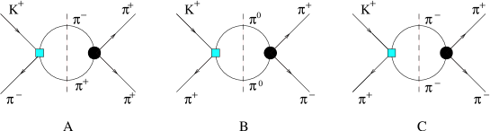
Figure 1: Relevant diagrams for the calculation of FSI for $K^{+}\rightarrow\pi^{+}\pi^{+}\pi^{-}$. The square vertex is the weak vertex and the round one is the strong vertex

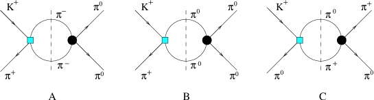
Figure 2: Relevant diagrams for the calculation of FSI for $K^{+}\rightarrow\pi^{0}\pi^{0}\pi^{+}$. The square vertex is the weak vertex and the round one is the strong vertex.

We can distinguish the cases in which the weak vertex is of ${\cal O}(p^{4})$ and the strong vertex of order ${\cal O}(p^{2})$ and the inverse case in which the weak vertex is of order ${\cal O}(p^{2})$ and the strong vertex of order ${\cal O}(p^{4})$. In this paper we will not consider the weak vertices generated by the electroweak penguin. In Subsection E.1 we provide some notation. In Subsections E.2 and E.3 we report the calculation for the charged Kaon decays. An example of the calculation of the integrals that must be performed is given in Subsection E.4. Finally, in Subsection E.5 we give analytical results for the strong phases at NLO.

E.1 Notation

In order to be concise we use the functions $M_{i}$ for the weak amplitudes given in [10]. We define

$$\widetilde{M}_{i}(s) = \int_{-1}^{1}d\cos\theta\;\left.M_{i}(a(s)+b(s)\cos\theta)\right|_{p^{4}}\,,$$ (146)

$$\widetilde{M}_{i}^{s}(s) = \int_{-1}^{1}d\cos\theta\;\left.(a(s)+b(s)\cos\theta)M_{i}(a(s)+b(s)\cos\theta)\right|_{p^{4}}\,,$$ (147)

$$\widetilde{M}_{i}^{ss}(s) = \int_{-1}^{1}d\cos\theta\;\left.(a(s)+b(s)\cos\theta)^{2}M_{i}(a(s)+b(s)\cos\theta)\right|_{p^{4}}\,,$$ (148)

$$a(s) = \frac{1}{2}(m_{K}^{2}+3m_{\pi}^{2}-s)\,,$$

$$b(s) = \frac{1}{2}\sqrt{(s-4m_{\pi}^{2})\left(s-2(m_{K}^{2}+m_{\pi}^{2})+\frac{(m_{K}^{2}-m_{\pi}^{2})^{2}}{s}\right)}\,.$$ (149)

The amplitudes at ${\cal O}(p^{4})$ for the $\pi\pi\rightarrow\pi\pi$ scattering in a theory with three flavors can be found in [59]. We decompose the amplitudes in the various cases as follows. For the case $\pi^{+}\pi^{+}\rightarrow\pi^{+}\pi^{+}$ the amplitude at ${\cal O}(p^{4})$ is

$$\Pi_{1} = P_{1}(s)+P_{2}(s,t)+P_{2}(s,u).$$ (150)

For the case $\pi^{0}\pi^{0}\rightarrow\pi^{+}\pi^{-}$ the amplitude at ${\cal O}(p^{4})$ is

$$\Pi_{2} = P_{3}(s)+P_{4}(s,t)+P_{4}(s,u).$$ (151)

For the case $\pi^{+}\pi^{-}\rightarrow\pi^{+}\pi^{-}$ the amplitude at ${\cal O}(p^{4})$ is

$$\Pi_{3} = P_{5}(s)+P_{6}(s,t)+P_{6}(s,u)+P_{7}(s,t)-P_{7}(s,u).$$ (152)

Finally the amplitude $\pi^{0}\pi^{0}\rightarrow\pi^{0}\pi^{0}$ at ${\cal O}(p^{4})$ is

$$\Pi_{4} = P_{8}(s)+P_{8}(t)+P_{8}(u).$$ (153)

The value for the various $P_{i}$ can be deduced from [59]. In the following we use

$$\!\!\!\!\!\!\!\!\!\widetilde{P}^{(n,m)}_{i}(s) = \int_{-1}^{1}d\cos\theta\;s^{n}(c(s)(1-\cos\theta))^{m}P_{i}(s,c(s)(1-\cos\theta))\,,$$ (154)

$$\!\!\!\!\!\!\!\!\!\widehat{P}^{(n)}_{1,i}(s) = \int_{-1}^{1}d\cos\theta\;(c(s)(1-\cos\theta))^{n}P_{i}(c(s)(1+\cos\theta),c(s)(1-\cos\theta))\,,$$ (155)

$$\!\!\!\!\!\!\!\!\!\widehat{P}^{(n)}_{2,i}(s) = \int_{-1}^{1}d\cos\theta\;(c(s)(1-\cos\theta))^{n}P_{i}(c(s)(1-\cos\theta),s)\,,$$ (156)

$$\!\!\!\!\!\!\!\!\!c(s) = -\frac{1}{2}(s-4m_{\pi}^{2})\,.$$ (157)

Another function we use in the next subsections is $\sigma(s)$ which was defined already in (144).

E.2 Final State Interactions for $K^{+}\rightarrow\pi^{+}\pi^{+}\pi^{-}$

We first compute the contributions depicted in Figure 1 in which the weak vertex is of ${\cal O}(p^{4})$ and the strong vertex of ${\cal O}(p^{2})$. The results for the diagrams A and B are

$${\rm Im}A^{(6,1)}_{W} = \frac{\sigma(s_{3})}{32\pi}\frac{(2m_{\pi}^{2}-s_{3})}{f_{\pi}^{2}}\left[\left.M_{10}(s_{3})\right|_{p^{4}}+\widetilde{M}_{11}(s_{3})+\widetilde{M}_{12}(s_{3})(m_{K}^{2}\right.$$ (158)

$$+3m_{\pi}^{2}-2s_{3})\left.-\widetilde{M}_{12}^{s}(s_{3})\right]\,,$$

$${\rm Im}A^{(6,2)}_{W} = \frac{\sigma(s_{1})}{32\pi}\frac{(s_{1}-m_{\pi}^{2})}{f_{\pi}^{2}}\left[\left.M_{7}(s_{1})\right|_{p^{4}}+\widetilde{M}_{8}(s_{1})+\widetilde{M}_{9}(s_{1})(m_{K}^{2}+3m_{\pi}^{2}-2s_{1})\right.$$ (159)

$$\left.-\widetilde{M}_{9}^{s}(s_{1})\right]+(s_{1}\leftrightarrow s_{2})\,,$$

respectively. For diagram C we have both $S$-wave and $P$-wave contributions. We get for them

$${\rm Im}A^{(6,3)}_{W,S} = \frac{\sigma(s_{1})}{64\pi}\frac{s_{1}}{f_{\pi}^{2}}\left[2\left.M_{11}(s_{1})\right|_{p^{4}}+\widetilde{M}_{11}(s_{1})+\widetilde{M}_{10}(s_{1})+\widetilde{M}_{12}^{s}(s_{1})\right.$$ (160)

$$\left.-\widetilde{M}_{12}(s_{1})(m_{K}^{2}+3m_{\pi}^{2}-2s_{1})\right]+(s_{1}\leftrightarrow s_{2})\,,$$

$${\rm Im}A^{(6,3)}_{W,P} = \frac{\sigma(s_{1})}{64\pi}\frac{1}{f_{\pi}^{2}}\frac{s_{1}(s_{3}-s_{2})}{s_{1}^{2}-2(m_{K}^{2}+m_{\pi}^{2})s_{1}+(m_{K}^{2}-m_{\pi}^{2})^{2}}\left[(s_{1}-(m_{K}^{2}+3m_{\pi}^{2}))\right.$$ (161)

$$\!\!\!\times(\widetilde{M}_{11}(s_{1})-\widetilde{M}_{10}(s_{1})+\widetilde{M}_{12}(s_{1})(2s_{1}-m_{K}^{2}-3m_{\pi}^{2}))+2\widetilde{M}^{s}_{11}(s_{1})$$

$$\!\!\!-2\widetilde{M}^{s}_{10}(s_{1})+\widetilde{M}^{s}_{12}(s_{1})(5s_{1}-3(m_{K}^{2}+3m_{\pi}^{2}))+2\widetilde{M}^{ss}_{12}(s_{1})$$

$$\!\!\!+\frac{8}{3}b^{2}(s_{1})\left.M_{12}(s_{1})\right|_{p^{4}}\Big{]}+(s_{1}\leftrightarrow s_{2})\,,$$

respectively.

Secondly, we report the calculation of the case in which the strong vertex is of ${\cal O}(p^{4})$ and the weak vertex is of ${\cal O}(p^{2})$. With analogous notation as above, we get

$${\rm Im}A^{(6,1)}_{\pi} = \frac{\sigma(s_{3})}{32\pi}\left.M_{10}(s_{3})\right|_{p^{2}}\ (P_{1}(s_{3})+\widetilde{P}^{(0,0)}_{2}(s_{3}))\,,$$ (162)

$${\rm Im}A^{(6,2)}_{\pi} = \frac{\sigma(s_{1})}{32\pi}\left.(M_{7}(s_{1})+M_{8}(s_{2})+M_{8}(s_{3}))\right|_{p^{2}}\,(P_{3}(s_{1})+\widetilde{P}^{(0,0)}_{4}(s_{1}))$$ (163)

$$\!\!\!+(s_{1}\leftrightarrow s_{2})\,,$$

$${\rm Im}A^{(6,3)}_{\pi,S} = \frac{\sigma(s_{1})}{32\pi}\left(\left.M_{10}(s_{3})\right|_{p^{2}}+\left.M_{10}(s_{2})\right|_{p^{2}}\right)(P_{5}(s_{1})+\widetilde{P}^{(0,0)}_{6}(s_{1}))$$ (164)

$$\!\!\!+(s_{1}\leftrightarrow s_{2})\,,$$

$${\rm Im}A^{(6,3)}_{\pi,P} = \frac{\sigma(s_{1})}{32\pi}\left(\left.M_{10}(s_{3})\right|_{p^{2}}-\left.M_{10}(s_{2})\right|_{p^{2}}\right)\frac{1}{s_{1}-4m_{\pi}^{2}}\Big{(}(s_{1}-4m_{\pi}^{2})\widetilde{P}_{7}^{(0,0)}(s_{1})$$ (165)

$$\!\!\!+2\widetilde{P}_{7}^{(0,1)}(s_{1})\Big{)}+(s_{1}\leftrightarrow s_{2})\,.$$

The final result for the Im$A^{(6)}$ is given by the sum

$${\rm Im}A^{(6)} = \sum_{i=1,2;\ j=W,\pi}{\rm Im}A^{(6,i)}_{j}+\sum_{j=W,\pi;\ k=S,P}{\rm Im}A^{(6,3)}_{j,k}\,.$$ (166)

The relation between this imaginary amplitude and the functions defined in Appendix B is

$$\mbox{Im }A^{(6)}=\sum_{i=8,27}G_{i}\,C_{i}^{(6)}(s_{1},s_{2},s_{3})\,+\,\sum_{i=1,11}H_{i}^{(6)}(s_{1},s_{2},s_{3})\widetilde{K}_{i}\,.$$ (167)

This relation is also valid for $K^{+}\to\pi^{0}\pi^{0}\pi^{+}$.

E.3 Final State Interactions for $K^{+}\rightarrow\pi^{0}\pi^{0}\pi^{+}$

The calculation is analogous to the one for $K^{+}\rightarrow\pi^{+}\pi^{+}\pi^{-}$. The relevant graphs are depicted in Figure 2. In the case in which the weak vertex is of ${\cal O}(p^{4})$, we get

$${\rm Im}A^{(6,1)}_{W} = \frac{\sigma(s_{3})}{32\pi}\frac{(s_{3}-m_{\pi}^{2})}{f_{\pi}^{2}}\left[2M_{11}(s_{3})+\widetilde{M}_{11}(s_{3})+\widetilde{M}_{10}(s_{3})-\widetilde{M}_{12}(s_{3})(m_{K}^{2}\right.$$ (168)

$$\left.+3m_{\pi}^{2}-2s_{3})+\widetilde{M}_{12}^{s}(s_{3})\right]\,,$$

$${\rm Im}A^{(6,2)}_{W} = \frac{\sigma(s_{3})}{32\pi}\frac{m_{\pi}^{2}}{f_{\pi}^{2}}\left[M_{7}(s_{3})+\widetilde{M}_{8}(s_{3})+\widetilde{M}_{9}(s_{3})(m_{K}^{2}+3m_{\pi}^{2}-2s_{3})\right.$$ (169)

$$\left.-\widetilde{M}_{9}^{s}(s_{3})\right]\,,$$

$${\rm Im}A^{(6,3)}_{W,S} = \frac{\sigma(s_{1})}{64\pi}\frac{(2m_{\pi}^{2}-s_{1})}{f_{\pi}^{2}}\left[2M_{8}(s_{1})+\widetilde{M}_{8}(s_{1})+\widetilde{M}_{7}(s_{1})-\widetilde{M}_{9}(s_{1})(m_{K}^{2}\right.$$ (170)

$$+3m_{\pi}^{2}-2s_{1})\left.+\widetilde{M}_{9}^{s}(s_{1})\right]+(s_{1}\leftrightarrow s_{2})\,.$$

Also in this case diagram C generates both $S$-wave and $P$-wave contributions. The P-wave contribution due to the diagram C in 2 is

$${\rm Im}A^{(6,3)}_{W,P} = \frac{\sigma(s_{1})}{64\pi}\frac{1}{f_{\pi}^{2}}\frac{s_{1}(s_{3}-s_{2})}{s_{1}^{2}-2(m_{K}^{2}+m_{\pi}^{2})s_{1}+(m_{K}^{2}-m_{\pi}^{2})^{2}}\left[(s_{1}-(m_{K}^{2}+3m_{\pi}^{2}))\right.$$ (171)

$$\!\!\!\times(\widetilde{M}_{8}(s_{1})-\widetilde{M}_{7}(s_{1})+\widetilde{M}_{9}(s_{1})(2s_{1}-m_{K}^{2}-3m_{\pi}^{2}))+2\widetilde{M}^{s}_{8}(s_{1})$$

$$\!\!\!-2\widetilde{M}^{s}_{7}(s_{1})+\widetilde{M}^{s}_{9}(s_{1})(5s_{1}-3(m_{K}^{2}+3m_{\pi}^{2}))+2\widetilde{M}^{ss}_{9}(s_{1})$$

$$\!\!\!+\frac{8}{3}b^{2}(s_{1})M_{9}(s_{1})\Big{]}+(s_{1}\leftrightarrow s_{2})\,.$$

If the strong vertex is ${\cal O}(p^{4})$ and the weak vertex is order ${\cal O}(p^{2})$, we get

$${\rm Im}A^{(6,1)}_{\pi} = \frac{\sigma(s_{3})}{32\pi}\left.(M_{10}(s_{1})+M_{10}(s_{2}))\right|_{p^{2}}\ (P_{3}(s_{3})+\widetilde{P}^{(0,0)}_{4}(s_{3}))\,,$$ (172)

$${\rm Im}A^{(6,2)}_{\pi} = \frac{\sigma(s_{3})}{32\pi}\left.(M_{7}(s_{3})+M_{8}(s_{1})+M_{8}(s_{2}))\right|_{p^{2}}\,(P_{8}(s_{3})+\widetilde{P}^{(0,0)}_{8}(s_{3}))\,,$$

$${\rm Im}A^{(6,3)}_{\pi,S} = \frac{\sigma(s_{1})}{64\pi}\left.\left(2M_{8}(s_{1})+M_{8}(s_{2})+M_{8}(s_{3})+M_{7}(s_{2})+M_{7}(s_{3})\right)\right|_{p^{2}}$$ (174)

$$\!\!\!\times\Big{(}\widetilde{P}^{(0,0)}_{3}(s_{1})+\widehat{P}^{(0)}_{1,4}(s_{1})+\widetilde{P}^{(0)}_{2,4}(s_{1})\Big{)}+(s_{1}\leftrightarrow s_{2})\,,$$

$${\rm Im}A^{(6,3)}_{\pi,P} = \frac{\sigma(s_{1})}{64\pi}\left.\left(M_{7}(s_{3})-M_{8}(s_{3})-M_{7}(s_{2})+M_{8}(s_{2})\right)\right|_{p^{2}}\frac{1}{s_{1}-4m_{\pi}^{2}}$$ (175)

$$\!\!\!\times\Big{(}(s_{1}-4m_{\pi}^{2})(\widetilde{P}^{(0,0)}_{3}(s_{1})-\widehat{P}^{(0)}_{1,4}(s_{1})+\widetilde{P}^{(0)}_{2,4}(s_{1}))+2\widetilde{P}^{(1,0)}_{3}(s_{1})$$

$$\!\!\!-2\widetilde{P}^{(1)}_{1,4}(s_{1})+2\widehat{P}^{(1)}_{2,4}(s_{1})\Big{)}+(s_{1}\leftrightarrow s_{2})\,.$$

The total contribution is given by the sum of (166) with the proper right-hand side terms.

E.4 Integrals

The integrals necessary to compute the two-bubble FSI we discussed in the previous subsection can be calculated generalizing the method outlined in [60]. As an example we show the integration of the function

$$32\pi^{2}B(m_{1},m_{2},t) = C_{B}+\left\{\frac{2\eta\delta}{t}\ln\frac{\eta-\delta}{\eta+\delta}+\frac{\lambda}{t}\ln\frac{(\lambda-t)^{2}-\eta^{2}\delta^{2}}{(\lambda+t)^{2}-\eta^{2}\delta^{2}}\right\}$$ (176)

where $C_{B}$ is a term which does not depend on $t$,

$$C_{B} = 2\left(1-\ln\frac{\eta^{2}-\delta^{2}}{4\nu^{2}}\right)$$ (177)

and

$$\eta = m_{1}+m_{2}$$

$$\delta = m_{1}-m_{2}$$

$$\lambda = \sqrt{\left[\left(t-\eta^{2}\right)\left(t-\delta^{2}\right)\right]}\,.$$ (178)

In the center of mass frame one can define

$$Q = p_{K}+p_{\pi}=(\sqrt{s},0,0,0)$$

$$p_{\pi} = \frac{\sqrt{s}}{2}\left(\left(1-\frac{m_{K}^{2}-m_{\pi}^{2}}{s}\right),0,0,\sqrt{1-\frac{2(m_{K}^{2}+m_{\pi}^{2})}{s}+\frac{(m_{K}^{2}-m_{\pi}^{2})^{2}}{s^{2}}}\right)$$

where $p_{\pi}$ is the momentum of the external pion entering in the same vertex of the Kaon. The functions $B$ can also be generated in the strong vertex. In this case $p_{k}$ is the momentum of an external pion. The contribution to the imaginary part of the amplitude $A$ is

$${\rm Im}\,A=\frac{1}{32\pi}\sigma(s)\int_{-1}^{1}{\rm d}\,\cos\theta\,B[m_{1},m_{2},t]$$ (180)

with

$$t = a+b\cos\theta$$ (181)

and $a\equiv a(s)$, $b\equiv b(s)$ in (146). In order to solve the difficult part of the integral one can put

$$t=\frac{1}{2}\left[\eta^{2}+\delta^{2}-(\eta^{2}-\delta^{2})\frac{1+x^{2}}{2x}\right]\,.$$ (182)

In this way

$$\int_{-1}^{1}d\!\cos\theta\frac{\lambda}{t}\ln\frac{(\lambda-t)^{2}-\eta^{2}\delta^{2}}{(\lambda+t)^{2}-\eta^{2}\delta^{2}} = \frac{\eta^{2}-\delta^{2}}{2b}\int_{x_{\rm min}}^{x_{\rm max}}dx\;\frac{(1-x^{2})^{2}\ln x}{x^{2}\left(x^{2}+1-2x\alpha\right)}$$ (184)

$$= \frac{\eta^{2}-\delta^{2}}{2bx}\biggr{\{}-1-x^{2}-(1-x^{2})\ln x+\alpha x\ln^{2}x$$

$$\!\!\!+2x\sqrt{\alpha^{2}-1}\biggl{(}\ln x\ln\frac{1-\alpha+x\sqrt{a^{2}-1}}{1-\alpha-x\sqrt{a^{2}-1}}\biggr{.}$$

$$\!\!\!+Li_{2}\left(\frac{x}{\alpha+\sqrt{\alpha^{2}-1}}\right)$$

$$\!\!\!\left.\biggl{.}+Li_{2}\left(x(\alpha+\sqrt{\alpha^{2}-1})\right)\biggr{)}\biggr{\}}\right|_{x_{\rm min}}^{x_{\rm max}}$$

where

$$\alpha = {(\eta^{2}+\delta^{2})\over(\eta^{2}-\delta^{2})}$$

$$x_{\rm max} = \frac{2}{\eta^{2}-\delta^{2}}\left\{\frac{\eta^{2}+\delta^{2}}{2}-a-b+\frac{1}{2}\sqrt{(2(a+b)-(\eta^{2}+\delta^{2}))^{2}-(\eta^{2}-\delta^{2})^{2}}\right\}$$

$$x_{\rm min} = \frac{2}{\eta^{2}-\delta^{2}}\left\{\frac{\eta^{2}+\delta^{2}}{2}-a+b+\frac{1}{2}\sqrt{(2(a-b)-(\eta^{2}+\delta^{2}))^{2}-(\eta^{2}-\delta^{2})^{2}}\right\}\,.$$

In the case $m_{K}=m_{\pi}$, $a+b=0$ and one recovers the formulas of [60].

E.5 Analytical Results for the Dominant FSI Phases at NLO

The elements of the matrices defined in (62) have the next analytical expressions at NLO

$$\mathbb{R}^{\rm LO} = \left(\begin{array}[]{cc}R_{11}&R_{12}\\ R_{21}&R_{22}\end{array}\right)\,,$$ (188)

$$\delta_{2}^{\rm NLO} = \frac{\displaystyle\sum_{i=8,27,E}G_{i}\left(C_{i,1}^{(++-)}+C_{i,1}^{(00+)}\right)+\sum_{i=1,11}\left(H_{i,1}^{(6)(++-)}+H_{i,1}^{(6)(00+)}\right)\widetilde{K}_{i}}{\displaystyle\sum_{i=8,27,E}G_{i}\left(B_{i,1}^{(++-)}+B_{i,1}^{(00+)}\right)+\sum_{i=1,11}\left(H_{i,1}^{(4)(++-)}+H_{i,1}^{(4)(00+)}\right)\widetilde{K}_{i}}\,,$$ (189)

with

$$R_{11} = \frac{\left(-\beta_{1}+\frac{1}{2}\beta_{3}\right)^{\rm NR}\left(\alpha_{1}+\alpha_{3}\right)^{\rm R-NR}-\left(\beta_{1}+\beta_{3}\right)^{\rm NR}\left(-\alpha_{1}+\frac{1}{2}\alpha_{3}\right)^{\rm R-NR}}{\left(-\beta_{1}+\frac{1}{2}\beta_{3}\right)^{\rm NR}\left(\alpha_{1}+\alpha_{3}\right)^{\rm NR}-\left(\beta_{1}+\beta_{3}\right)^{\rm NR}\left(-\alpha_{1}+\frac{1}{2}\alpha_{3}\right)^{\rm NR}}\,,$$

$$R_{21} = \frac{\left(-\beta_{1}+\frac{1}{2}\beta_{3}\right)^{\rm NR}\left(\beta_{1}+\beta_{3}\right)^{\rm R-NR}-\left(\beta_{1}+\beta_{3}\right)^{\rm NR}\left(-\beta_{1}+\frac{1}{2}\beta_{3}\right)^{\rm R-NR}}{\left(-\beta_{1}+\frac{1}{2}\beta_{3}\right)^{\rm NR}\left(\alpha_{1}+\alpha_{3}\right)^{\rm NR}-\left(\beta_{1}+\beta_{3}\right)^{\rm NR}\left(-\alpha_{1}+\frac{1}{2}\alpha_{3}\right)^{\rm NR}}\ ,$$

$$R_{12} = -\frac{\left(-\alpha_{1}+\frac{1}{2}\alpha_{3}\right)^{\rm NR}\left(\alpha_{1}+\alpha_{3}\right)^{\rm R-NR}-\left(\alpha_{1}+\alpha_{3}\right)^{\rm NR}\left(-\alpha_{1}+\frac{1}{2}\alpha_{3}\right)^{\rm R-NR}}{\left(-\beta_{1}+\frac{1}{2}\beta_{3}\right)^{\rm NR}\left(\alpha_{1}+\alpha_{3}\right)^{\rm NR}-\left(\beta_{1}+\beta_{3}\right)^{\rm NR}\left(-\alpha_{1}+\frac{1}{2}\alpha_{3}\right)^{\rm NR}}\,,$$

$$R_{22} = -\frac{\left(-\alpha_{1}+\frac{1}{2}\alpha_{3}\right)^{\rm NR}\left(\beta_{1}+\beta_{3}\right)^{\rm R-NR}-\left(\alpha_{1}+\alpha_{3}\right)^{\rm NR}\left(-\beta_{1}+\frac{1}{2}\beta_{3}\right)^{\rm R-NR}}{\left(-\beta_{1}+\frac{1}{2}\beta_{3}\right)^{\rm NR}\left(\alpha_{1}+\alpha_{3}\right)^{\rm NR}-\left(\beta_{1}+\beta_{3}\right)^{\rm NR}\left(-\alpha_{1}+\frac{1}{2}\alpha_{3}\right)^{\rm NR}}\,,$$ (190)

The definitions of $\alpha_{1}$, $\alpha_{3}$, $\beta_{1}$ and $\beta_{3}$ are in (6.1) and the values of their relevant combinations are

$$\left(-\alpha_{1}+\frac{1}{2}\alpha_{3}\right)^{\rm NR} = \sum_{i=8,27,E}G_{i}B_{i,0}^{(00+)}+\sum_{i=1,11}H_{i,0}^{(4)(00+)}\widetilde{K}_{i}\,,$$

$$\left(-\alpha_{1}+\frac{1}{2}\alpha_{3}\right)^{\rm R-NR} = \sum_{i=8,27,E}G_{i}C_{i,0}^{(00+)}+\sum_{i=1,11}H_{i,0}^{(6)(00+)}\widetilde{K}_{i}\,,$$

$$\left(-\beta_{1}+\frac{1}{2}\beta_{3}\right)^{\rm NR} = \frac{1}{2}\left[\sum_{i=8,27,E}G_{i}\left(B_{i,1}^{(++-)}-B_{i,1}^{(00+)}\right)\right.$$

$$\left.+\sum_{i=1,11}\left(H_{i,1}^{(4)(++-)}-H_{i,1}^{(4)(00+)}\right)\widetilde{K}_{i}\right]\,,$$

$$\left(-\beta_{1}+\frac{1}{2}\beta_{3}\right)^{\rm R-NR} = \frac{1}{2}\left[\sum_{i=8,27,E}G_{i}\left(C_{i,1}^{(++-)}-C_{i,1}^{(00+)}\right)\right.$$

$$\left.+\sum_{i=1,11}\left(H_{i,1}^{(6)(++-)}-H_{i,1}^{(6)(00+)}\right)\widetilde{K}_{i}\right]\,,$$

$$\left(\alpha_{1}+\alpha_{3}\right)^{\rm NR} = \sum_{i=8,27,E}G_{i}B_{i,0}^{(+-0)}+\sum_{i=1,11}H_{i,0}^{(4)(+-0)}\widetilde{K}_{i}\,,$$

$$\left(\alpha_{1}+\alpha_{3}\right)^{\rm R-NR} = \sum_{i=8,27,E}G_{i}C_{i,0}^{(+-0)}+\sum_{i=1,11}H_{i,0}^{(6)(+-0)}\widetilde{K}_{i}\,,$$

$$\left(\beta_{1}+\beta_{3}\right)^{\rm NR} = -\frac{1}{2}\left[\sum_{i=8,27,E}G_{i}B_{i,1}^{(+-0)}+\sum_{i=1,11}H_{i,1}^{(4)(+-0)}\widetilde{K}_{i}\right]\,,$$

$$\left(\beta_{1}+\beta_{3}\right)^{\rm R-NR} = \frac{1}{2}\left[\sum_{i=8,27,E}G_{i}C_{i,1}^{(+-0)}+\sum_{i=1,11}H_{i,1}^{(6)(+-0)}\widetilde{K}_{i}\right]\,.$$ (191)

where the functions $B_{i,0(1)}$, $C_{i,0(1)}$ and $H_{i,0(1)}$ are those obtained form the expansion in (106) of the corresponding full quantities that can be found in Appendix D.

Disregarding the tiny CP-violating (less than 1%) and the effects of order $e^{2}p^{2}$ (the loop contribution is less than 2%), we obtain the numbers in (6.1).

References

[1]
J.A. Cronin,
Phys. Rev. 161 (1967) 1483;
B.R. Holstein,
ibidem 183 (1969) 1228;
T.J. Devlin and J.O. Dickey,
Rev. Mod. Phys. 51 (1979) 237.
[2] S. Weinberg,
Physica A 96 (1979) 327.
[3]
J. Gasser and H. Leutwyler,
Annals Phys. 158 (1984) 142;
Nucl. Phys. B 250 (1985) 465.
[4]
J.F. Donoghue, E. Golowich, B.R. Holstein,
Phys. Rev. D 30 (1984) 587;
H.-Y. Cheng, C.Y. Cheung, W.B. Yeung,
Mod. Phys. Lett. A 4 (1989) 869;
Z. Phys. C 43 (1989) 391;
S. Fajfer, J.-M. Gérard,
Z. Phys. C 42 (1989) 425.
[5] G. Ecker, arXiv:hep-ph/0011026;
A. Pich, arXiv:hep-ph/9806303.
[6]
G. Ecker,
Prog. Part. Nucl. Phys. 35 (1995) 1
[arXiv:hep-ph/9501357];
E. de Rafael,
arXiv:hep-ph/9502254;
A. Pich,
Rept. Prog. Phys. 58 (1995) 563
[arXiv:hep-ph/9502366].
[7]
J. Kambor, J. Missimer and D. Wyler,
Phys. Lett. B 261 (1991) 496.
[8]
J. Kambor, J. Missimer and D. Wyler,
Nucl. Phys. B 346 (1990) 17.
[9]
J. Kambor, J.F. Donoghue, B.R. Holstein, J. Missimer and D. Wyler,
Phys. Rev. Lett. 68 (1992) 1818.
[10]
J. Bijnens, P. Dhonte and F. Persson,
Nucl. Phys. B 648 (2003) 317
[arXiv:hep-ph/0205341].
[11]
B.R. Holstein
Phys. Rev. 177 (1969) 2417.
[12]
L.-F. Li and L. Wolfenstein,
Phys. Rev. D 21 (1980) 178.
[13]
C. Avilez,
Phys. Rev. D 23 (1981) 1124.
[14]
B. Grinstein, S.-J. Rey and M.B. Wise,
Phys. Rev. D 33 (1986) 1495.
[15]
J.F. Donoghue, B.R. Holstein and G. Valencia,
Phys. Rev. D 36 (1987) 798.
[16]
A.A. Bel’kov, A.V. Lanyov, G. Bohm and D. Ebert,
Phys. Lett. B 232 (1989) 118;
A.A. Bel’kov, G. Bohm, D. Ebert, A.V. Lanyov and A. Schaale,
Int. J. Mod. Phys. A 7 (1992) 4757.
[17]
G. D’Ambrosio, G. Isidori and N. Paver,
Phys. Lett. B 273 (1991) 497.
[18]
G. Isidori, L. Maiani and A. Pugliese,
Nucl. Phys. B 381 (1992) 522.
[19]
L. Maiani and N. Paver,
The Second DANE Physics Handbook,
Vol. I (1995) p. 51, L. Maiani, G. Pancheri and N. Paver (ed).
[22]
G. D’Ambrosio, G. Isidori, A. Pugliese and N. Paver,
Phys. Rev. D 50 (1994) 5767
[Erratum-ibid. D 51 (1995) 3975]
[arXiv:hep-ph/9403235].
[23]
I.V. Ajinenko et al.,
Phys. Lett. B 567 (2003) 159
[arXiv:hep-ex/0205027].
[24] R. Wanke,
arXiv:hep-ex/0305059;
C. Cheshkov,
arXiv:hep-ex/0306012.
[25]
A. Aloisio et al. [KLOE Collaboration],
arXiv:hep-ex/0307054;
M. Primavera, Talk at Workshop on Chiral Dynamics 2003: Theory
and Experiment, Bonn, Germany, September 8-13 (2003).
[26]
E. Gámiz, J. Prades and I. Scimemi,
arXiv:hep-ph/0305164.
[27]
J. Bijnens, E. Pallante and J. Prades,
Nucl. Phys. B 521 (1998) 305
[arXiv:hep-ph/9801326].
[28]
K. Schubert, Plenary talk at 21st International
Symposium on Lepton and Photon Interactions at High
Energies, Fermilab, Batavia, IL, USA, August 11-16 (2003).
[29]
J. Bijnens, J. Prades and E. de Rafael,
Phys. Lett. B 348 (1995) 226;
[arXiv:hep-ph/9411285]
J. Prades,
Nucl. Phys. B (Proc. Suppl.) 64 (1998) 253
[arXiv:hep-ph/9708395].
[30]
M. Jamin,
Phys. Lett. B 538 (2002) 71
[arXiv:hep-ph/0201174];
M. Jamin, J.A. Oller and A. Pich,
Eur. Phys. J. C 24 (2002) 237
[arXiv:hep-ph/0110194];
K. Maltman and J. Kambor,
Phys. Lett. B 517 (2001) 332
[arXiv:hep-ph/0107060].
[31]
H. Wittig,
arXiv:hep-lat/0210025.
[32]
V. Cirigliano, J.F. Donoghue, E. Golowich and K. Maltman,
Phys. Lett. B 555 (2003) 71
[arXiv:hep-ph/0211420];
arXiv:hep-ph/0209332;
Phys. Lett. B 522 (2001) 245
[arXiv:hep-ph/0109113];
J.F. Donoghue and E. Golowich,
Phys. Lett. B 478 (2000) 172
[arXiv:hep-ph/9911309].
[33]
S. Narison,
Nucl. Phys. B 593 (2001) 3
[arXiv:hep-ph/0004247].
[34]
J. Bijnens, E. Gámiz and J. Prades,
J. High Energy Phys. 10 (2001) 009
[arXiv:hep-ph/0108240];
E. Gámiz, J. Prades and J. Bijnens,
Nucl. Phys. B (Proc. Suppl.) 126 (2003) 195
[arXiv:hep-ph/0209089].
[35]
R. Barate et al, [ALEPH Collaboration]
Eur. Phys. J. C 4 (1998) 409.
[36]
K. Ackerstaff et al. [OPAL Collaboration],
Eur. Phys. J. C 7 (1999) 571
[arXiv:hep-ex/9808019].
[37]
M. Knecht, S. Peris and E. de Rafael,
Phys. Lett. B 508 (2001) 117
[arXiv:hep-ph/0102017];
Phys. Lett. B 457 (1999) 227
[arXiv:hep-ph/9812471].
[38]
J.I. Noaki et al. [CP-PACS Collaboration],
Phys. Rev. D 68 (2003) 014501
[arXiv:hep-lat/0108013],
Nucl. Phys. B (Proc. Suppl.) 106 (2002) 332
[arXiv:hep-lat/0110142];
T. Blum et al. [RBC Collaboration],
arXiv:hep-lat/0110075,
Nucl. Phys. B (Proc. Suppl.) 106 (2002) 317
[arXiv:hep-lat/0110185].
[39]
D. Bećirević et al. [SPQCDR Collaboration],
arXiv:hep-lat/0209136.
[40]
J. Bijnens and J. Prades,
J. High Energy Phys. 06 (2000) 035
[arXiv:hep-ph/0005189];
Nucl. Phys. B (Proc. Suppl.) 96 (2001) 354
[arXiv:hep-ph/0010008];
arXiv:hep-ph/0009156;
arXiv:hep-ph/0009155.
[41]
J. Bijnens and J. Prades,
J. High Energy Phys. 01 (1999) 023
[arXiv:hep-ph/9811472];
J. Prades,
Nucl. Phys. B (Proc. Suppl.) 86 (2000) 294
[arXiv:hep-ph/9909245].
[42]
S. Peris, M. Perrottet and E. de Rafael,
J. High Energy Phys. 05 (1998) 011.
[arXiv:hep-ph/9805442].
[43]
J. Bijnens, E. Gámiz, E. Lipartia and J. Prades,
J. High Energy Phys. 04 (2003) 055
[arXiv:hep-ph/0304222].
[44]
T. Hambye, S. Peris and E. de Rafael,
J. High Energy Phys. 05 (2003) 027
[arXiv:hep-ph/0305104].
[45]
T. Hambye, G.O. Köhler, E.A. Paschos and P.H. Soldan,
Nucl. Phys. B 564 (2000) 391
[arXiv:hep-ph/9906434];
T. Hambye, G.O. Köhler, E.A. Paschos, P.H. Soldan and W.A. Bardeen,
Phys. Rev. D 58 (1998) 014017
[arXiv:hep-ph/9802300].
[46]
G. Isidori and A. Pugliese,
Nucl. Phys. B 385 (1992) 437.
[47]
G. Ecker, J. Gasser, H. Leutwyler, A. Pich and E. de Rafael,
Phys. Lett. B 223 (1989) 425.
G. Ecker, J. Gasser, A. Pich and E. de Rafael,
Nucl. Phys. B 321 (1989) 311.
[48]
E. Pallante, A. Pich and I. Scimemi,
Nucl. Phys. B 617 (2001) 441
[arXiv:hep-ph/0105011];
E. Pallante and A. Pich,
Nucl. Phys. B 592 (2001) 294
[arXiv:hep-ph/0007208];
Phys. Rev. Lett. 84 (2000) 2568
[arXiv:hep-ph/9911233].
[49]
M. Knecht and A. Nyffeler,
Eur. Phys. J. C 21 (2001) 659
[arXiv:hep-ph/0106034].
[50]
V. Cirigliano, G. Ecker, H. Neufeld and A. Pich,
J. High Energy Phys. 06 (2003) 012
[arXiv:hep-ph/0305311] and work in preparation.
[51]
M. Knecht, S. Peris and E. de Rafael,
Nucl. Phys. B (Proc. Suppl.) 86 (2000) 279
[arXiv:hep-ph/9910396].
[52]
K. Hagiwara et al. [Particle Data Group Collaboration],
Phys. Rev. D 66 (2002) 010001.
[53]
G. D’Ambrosio and G. Isidori,
Int. J. Mod. Phys. A 13 (1998) 1
[arXiv:hep-ph/9611284].
[54]
G. D’Ambrosio, G. Isidori and G. Martinelli,
Phys. Lett. B 480 (2000) 164
[arXiv:hep-ph/9911522].
[55]
G. Esposito-Farèse,
Z. Phys. C 50 (1991) 255.
[56]
G. Ecker, J. Kambor and D. Wyler,
Nucl. Phys. B 394 (1993) 101.
[57]
G. Ecker, G. Isidori, G. Müller, H. Neufeld and A. Pich,
Nucl. Phys. B 591 (2000) 419
[arXiv:hep-ph/0006172].
[58]
G. Amorós, J. Bijnens and P. Talavera,
Nucl. Phys. B 568 (2000) 319
[arXiv:hep-ph/9907264].
[59]
V. Bernard, N. Kaiser and U.-G. Meißner,
Nucl. Phys. B 357 (1991) 129.
[60]
J. Bijnens, G. Colangelo, G. Ecker, J. Gasser and M.E. Sainio,
Nucl. Phys. B 508 (1997) 263
[Erratum-ibid. B 517 (1998) 639]
[arXiv:hep-ph/9707291].