WUB 03-10
ITP-BUDAPEST 601
DESY 03-114
hep-ph/0309171

Bounds on the cosmogenic neutrino flux

Under the assumption that some part of the observed highest energy cosmic rays consists of protons originating from cosmological distances, we derive bounds on the associated flux of neutrinos generated by inelastic processes with the cosmic microwave background photons. We exploit two methods. First, a power-like injection spectrum is assumed. Then, a model-independent technique, based on the inversion of the observed proton flux, is presented. The inferred lower bound is quite robust. As expected, the upper bound depends on the unknown composition of the highest energy cosmic rays. Our results represent benchmarks for all ultrahigh energy neutrino telescopes.

1 Introduction

Ultrahigh energy cosmic ray (UHECR) protons with energies above the Greisen-Zatsepin-Kuzmin (GZK) cutoff, $E\,\raise 1.29167pt\hbox{$>$\kern-7.5pt\raise-4.73611pt\hbox{$\sim$}}\,E_{\rm GZK}=4\times 10^{19}$ eV, interact inelastically with the photons of the cosmic microwave background (CMB) and produce pions. This process results in a significant energy loss and an attenuation length of about $50$ Mpc. If the highest energy cosmic rays are protons and originate from distances beyond that scale, one expects a sharp drop in the observed spectrum at around $E_{\rm GZK}$ [1]. This GZK phenomenon also predicts a guaranteed ultrahigh energy neutrino flux, since the produced pions finally mainly decay into neutrinos [2]. These neutrinos are called GZK or cosmogenic neutrinos.

There are a number of estimates [2, 3] and upper bounds [4, 5, 6] on the cosmogenic neutrino fluxes, the most recent results being found in Refs. [7, 8, 9, 10, 11]. We summarized these predictions in Fig. 1. Surprisingly, one finds two orders of magnitude uncertainty due to the huge differences between the individual results. Present and future experiments need a clear picture of this phenomenon. Therefore, we present in this Letter a systematic quantitative analysis of the minimal and maximal expected cosmogenic neutrino fluxes. The only assumption we make is that some part of the observed highest energy cosmic rays consists of protons from cosmological distances. We include all cosmological and observational uncertainties into our calculation.

The inferred lower bounds on the cosmogenic neutrino fluxes turn out to be quite robust. These bounds are of particular interest. First of all, they represent benchmarks for all neutrino telescopes and cosmic ray facilities designed to be sensitive in the ultrahigh energy region (for a recent review, see Ref. [17]). Moreover, the lower bound on the flux can be turned into an upper bound on the neutrino nucleon cross-section, if no quasi-horizontal or deeply-penetrating air showers are observed [18]. This knowledge gives important information about a possible enhancement of the cross-sections in the multi-TeV centre-of-mass energy regime [19], which is expected in many standard model (SM) like or beyond the SM scenarios.

Our Letter is organized as follows. In Section 2, we summarize how the propagation of protons through the CMB and the associated production of neutrinos can be described by means of propagation functions. Section 3 presents two techniques to give upper and lower bounds on the cosmogenic neutrino fluxes. In Section 4 we conclude.

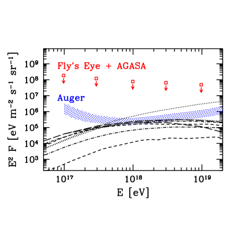
Figure 1: Various predictions for the cosmogenic neutrino fluxes. We assume full mixing between the flavours [12], and the presented results correspond to one flavour, $F_{\nu_{\ell}}+F_{\bar{\nu}_{\ell}}$, $\ell=e,\mu,\tau$. Lower (upper) short dashed line: flux from Ref. [7] for redshift evolution parameters (cf. Eq. (2)) $n=2$, $z_{\rm max}=2$ ($n=4$, $z_{\rm max}=4$). Lower (upper) long dashed line: flux from Ref. [8], assuming a maximum energy of $E_{\rm max}=3\times 10^{20(21)}$ eV for the ultrahigh energy cosmic protons (cf. Eq. (4)). Lower (upper) dashed dotted line: flux from Ref. [9], assuming $n=3$ ($n=4$). Lower and upper dotted line: flux from Ref. [10], assuming $(E_{\rm max},\alpha,n)=(1\times 10^{21}$ eV,$1.5,3)$ and $(3\times 10^{22}$ eV,$1.0,3)$, respectively, where $\alpha$ denotes the proton injection spectral index (cf. Eq. (4)). Boxes show the upper bounds obtained by combining Fly’s Eye [13] and Agasa [14] limits on deeply-penetrating showers in different energy bins [15]. The dotted band labelled by Auger represents the expected sensitivity of the Pierre Auger Observatory to $\nu_{\tau}+\bar{\nu}_{\tau}$, corresponding to one event per year per energy decade [16].

2 Propagation functions

Protons propagating from cosmological distances lose their energies by three basic processes. Above the GZK cutoff, the dominant particle physics process is scattering on the CMB through pion production. The produced pions decay, giving rise to the cosmogenic neutrinos. For proton energies between $10^{18}$ eV and the GZK cutoff, the dominant particle physics process is scattering on the CMB through $e^{+}e^{-}$ pair production. The expansion of the universe redshifts all the travelling particles, which is particularly important for protons produced at large distances.

The propagation of the proton toward the earth can be easily described [14, 20] by one single function $P_{p|p}(E;E_{i},r)$, which tells the probability that a proton created at distance $r$ with energy $E_{i}$ is detected on earth as a proton with energy above $E$. This probability function was calculated in Ref. [21] for a large range of $E,E_{i}$ and $r$. More generally, including other particle species, the effects of the propagation can be described [22, 11, 23] by $P_{b|a}(E;E_{i},r)$ functions, which give the expected number of particles of type $b$ above the threshold energy $E$ if one particle of type $a$ started at a distance $r$ with energy $E_{i}$.

In this Letter, we assume that the sources of the ultrahigh energy protons (nucleons) are isotropically distributed and can be described by a comoving luminosity distribution ${\mathcal{L}}_{p}(r,E_{i})$ of protons injected with energy $E_{i}$ at a distance $r$ from earth, which gives the number of protons per unit of comoving volume, per unit of time, and per unit of energy. With the help of the above propagation functions, one can calculate the differential flux of protons ($b=p$) and cosmogenic neutrinos ($b=\nu_{\ell},\bar{\nu}_{\ell}$) at earth. Their number $N_{b}$ arriving at earth with energy $E$ per units of energy, area ($A$), time ($t$) and solid angle ($\Omega$), can be expressed as

$$F_{b}(E)\equiv\frac{{\rm d}^{4}N_{b}}{{\rm d}E\,{\rm d}A\,{\rm d}t\,{\rm d}\Omega}=\frac{1}{4\pi}\,\int_{0}^{\infty}{\rm d}E_{i}\int_{0}^{\infty}{\rm d}r\,(-)\frac{\partial P_{b|p}(E;E_{i},r)}{\partial E}\,{\mathcal{L}}_{p}(r,E_{i})\,.$$ (1)

Note, that this formula can be easily generalized to arbitrary source luminosity distributions. In the following, we make the usual assumption [7, 8, 9, 10, 11] that the $r$ and $E_{i}$ dependences of the source luminosity distribution factorize, ${\mathcal{L}}_{p}(r,E_{i})=\rho(r)\,J_{p}(E_{i})$, and that the redshift evolution of the sources can be parametrized by a simple power-law,

$${\mathcal{L}}_{p}(r,E_{i})=\rho_{0}\,\left(1+z(r)\right)^{n}\,\theta(z-z_{\rm min})\,\theta(z_{\rm max}-z)\,J_{p}(E_{i})\,,$$ (2)

where the redshift $z$ and the distance $r$ are related by ${\rm d}z=(1+z)\,H(z)\,{\rm d}r$. We use the expression

$$H^{2}(z)=H_{0}^{2}\,\left[\Omega_{M}\,(1+z)^{3}+\Omega_{\Lambda}\right]$$ (3)

to relate the Hubble expansion rate at redshift $z$ with the present one. Uncertainties of the latter, $H_{0}=h$ 100 km/s/Mpc, with $h=(0.71\pm 0.07)\times^{1.15}_{0.95}$ [24], do not affect our results significantly. In Eq. (3), $\Omega_{M}$ and $\Omega_{\Lambda}$, with $\Omega_{M}+\Omega_{\Lambda}=1$, are the present matter and vacuum energy densities in terms of the critical density. As default values, we choose $\Omega_{M}=0.3$ and $\Omega_{\Lambda}=0.7$, which is favoured today. Our results turn out to be quite insensitive to the precise values of the cosmological parameters within their uncertainties. The universe is homogeneous for distances above the GZK scale ($50$ Mpc). The events between $10^{18}$ eV and the GZK cutoff are believed to come from cosmological distance. Therefore, it is physically motivated to use the ansatz (2) for the evolution of the luminosity of sources in addition to the pure redshifting ($n=0$). We set minimal and maximal redshift values by $z_{\rm min}$ and $z_{\rm max}$. These parameters exclude the existence of nearby and early time sources. We take $z_{\rm min}=0.012$, corresponding to $r_{\rm min}=50$ Mpc. The effects due to a change in $z_{\rm max}$ can be compensated by a change in $n$. Therefore, we fix $z_{\rm max}=2$ in the following and study the dependencies on $n$ only.

We neglect the effects of possible magnetic fields. They just deflect the trajectories of the protons and, thus, only increase the path length (synchrotron radiation of protons can be neglected). As long as the correlation length of the magnetic fields is smaller than the gyroradius of the protons (which holds for an anticipated magnetic field strength of $\approx$ nG), this effect is on the percent level, smaller than other uncertainties.

The details of our calculation of the $P_{b|a}(E;E_{i},r)$ functions for protons, neutrinos, charged leptons, and photons will be published elsewhere [23]. In short (see also Ref. [11]), we calculated $P_{b|a}(E;E_{i},r)$ in two steps. i) First, the SOPHIA Monte-Carlo program [25] was used for the simulation of photohadronic processes of protons with the CMB photons. For $e^{+}e^{-}$ pair production, we used the continuous energy loss approximation, since the inelasticity is very small ($\approx 10^{-3}$). We calculated the $P_{b|a}$ functions for “infinitesimal” steps ($1\div 10$ kpc) as a function of the redshift $z$. ii) We multiplied the corresponding infinitesimal probabilities starting at a distance $r(z)$ down to earth with $z=0$.

The determination of the propagation functions took approximately one day on an average personal computer. The advantage of the formulation of the spectra (1) in terms of the propagation functions is evident. The latter have to be determined only once and for all. Without the use of the propagation functions, one would have to perform a simulation for any variation of the source luminosity distribution ${\mathcal{L}}_{p}(r,E_{i})$, which requires excessive computer power. Since the propagation functions are of universal usage, we decided to make the latest versions of $-\partial P_{b|a}/\partial E$ available for the public via the World-Wide-Web URL www.desy.de/~uhecr  .

3 Bounds on the cosmic neutrino flux

In this Section, we present two techniques to derive robust upper and lower bounds on the cosmogenic neutrino fluxes.

The first technique assumes an $E_{i}^{-\alpha}$ power-like injection spectrum for the protons, with some maximal cutoff energy $E_{\rm max}$. A comparison of the spectrum after propagation with the observations allows to determine the confidence region for the power $\alpha$ and for the redshift evolution index $n$. Since the propagation of the protons leads to neutrino production, we may then infer the neutrino fluxes suggested by the different ($\alpha,n$) regions.

The second technique is based on an inversion of the observed proton flux around the GZK cutoff with the help of the proton’s propagation function. Though the inverted proton spectrum has non-negligible uncertainties, the inferred fluxes of the cosmogenic neutrinos are rather stable. We study the sensitivity of the resulting flux on the cosmological evolution parameter $n$.

The lower bounds for the neutrino fluxes obtained by these two techniques are in complete agreement. Since the post-GZK events can only be taken into account in the second method, the corresponding upper bound is larger than the one obtained by means of the first method.

3.1 Power-like injection spectrum

We assume an $E_{i}^{-\alpha}$ power-like injection spectrum for the protons,

$$J_{p}(E_{i})=J_{0}\,E^{-\alpha}_{i}\,\theta(E_{\rm max}-E_{i})\,,$$ (4)

up to $E_{\rm max}$, the maximal energy which can be reached through astrophysical accelerating processes in a bottom-up scenario. The normalization factors $J_{0}$ of the injection spectrum (4) and $\rho_{0}$ of the source distribution in Eq. (2) are fixed by the observed cosmic ray flux. The predicted differential proton flux at earth, Eq. (1), with this injection spectrum, is compared with the observations. A fitting procedure gives the most probable values for $E_{\rm max}$, $\alpha$ and $n$.

We quantify the goodness of our results by statistical methods. Our analysis is similar to that of Ref. [11]. It was carried out in two basic steps.

i) First we determined the number of experimentally observed events in a given energy bin by converting the published values of the cosmic ray flux. This had to be done, since the UHECR collaborations give their results for the observed flux in a binned form, whereas the number of events in a given bin is integer and follows the Poisson distribution. We analyzed the results from different experimental settings separately and performed the analysis for the two most recent results from the AGASA [26] and HiRes [27] collaborations. In the low energy region, there are no published results available from AGASA and only low statistics results from HiRes-2. Therefore, we included the results of the predecessor collaborations – Akeno [28] and Fly’s Eye [29] – into the analysis. With a small normalization correction, it was possible to continuously connect the AGASA data with the Akeno ones and the HiRes-1 monocular data with the Fly’s Eye stereo ones, respectively (cf. Fig. 3 (left)). The normalization was matched at $E=10^{18.5}$ eV for both cases.

ii) We determined the 2-sigma confidence regions in the $\alpha$–$n$ plane for each $E_{\rm max}$. In order to do that, we checked the compatibility of different ($\alpha,n$) pairs at a given $E_{\rm max}$ with the observed data. In this analysis, we used the energy range between $E_{-}=10^{17.2\div 18.5}$ eV and $E_{+}=10^{20}$ eV. The data in the bins above $10^{20}$ eV are not used, since events beyond the GZK cutoff can not be explained by just one power law injection spectrum with spectral index $\alpha$. This obvious statement can be formulated quantitatively. Using $z_{\rm min}=0.012$ (which reflects the observation that there are no UHECR sources within $r_{\rm min}\approx 50$ Mpc), we find that the data above $10^{20}$ eV are incompatible on the 3-sigma level with a pure power law fit in the energy region between $E_{-}=10^{17.2\div 18.5}$ eV and $E_{+}>10^{20}$ eV (see also Ref. [30]).

The compatibility of a given ($\alpha,n$) pair with the observational data was checked as follows. For some specific ($\alpha,n$) pair, the expected number of events in individual bins is calculated (${\bf\lambda}=\{\lambda_{1},...,\lambda_{r}\}$, where the $\lambda_{i}$’s are non-negative, usually non-integer numbers, and $r$ is the number of the bins). The probability distribution in the $i$-th bin is given by the Poisson distribution with mean $\lambda_{i}$. The $r$ dimensional probability distribution $P({\bf k})$ is just the product of the individual Poisson distributions (here ${\bf k}=\{k_{1},...k_{r}\}$ is a set of non-negative integer numbers). It is easy to include also the $\approx 30\%$ overall uncertainty in the energy measurement of the experiments into the $P({\bf k})$ probability. According to the $r$ dimensional probability distribution, the experimental result ${\bf s}=\{s_{1},...s_{r}\}$ (where the $s_{i}$’s are non-negative, integer numbers), has a definite, though usually very small probability $P({\bf s})$. The ($\alpha,n$) pair is compatible with the experimental results at the 2-sigma level if

$$\sum_{{\bf k}|P({\bf k})>P({\bf s})}P({\bf k})<0.95\,.$$ (5)

The best fit is found by minimizing the sum on the left hand side. This technique is equivalent to the $\chi^{2}$ technique for a large class of problems.

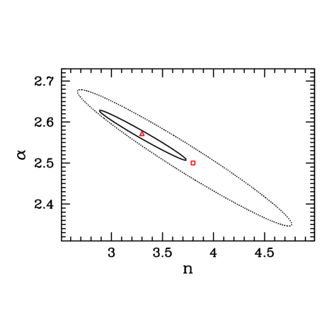
Figure 2: Two-sigma confidence regions in the power-law index $\alpha$ and the redshift evolution index $n$ plane. Results obtained with the Akeno + AGASA data are shown by a solid curve, whereas the results from Fly’s Eye + HiRes data are given by the dotted line. The triangle (square) represents the best fit values for AGASA (HiRes). The analysis used the data between energy bins $E_{-}=10^{17.2}$ eV and $E_{+}=10^{20}$ eV. Other parameters were $E_{\rm max}=3\times 10^{21}$ eV, $z_{\rm min}=0.012$, and $z_{\rm max}=2$.

For $E_{-}=10^{17.2}$ eV and $E_{+}=10^{20}$ eV, our best fit values are $E_{\rm max}=3\times 10^{21}$ eV, $\alpha=2.57$, $n=3.30$, for AGASA, and $E_{\rm max}=3\times 10^{21}$ eV, $\alpha=2.50$, $n=3.80$, for HiRes. Figure 2 displays the 2-sigma confidence regions in the $\alpha-n$ plane with $E_{\rm max}=3\times 10^{21}$ eV for both experiments. Figure 3 (left) shows our best fits to the Akeno + AGASA (top) and to the Flys’s Eye + HiRes (bottom) UHECR data. Fig. 3 (right) shows the resulting neutrino fluxes per flavour, assuming full mixing at arrival at earth [12].

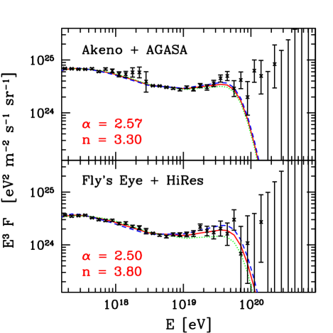
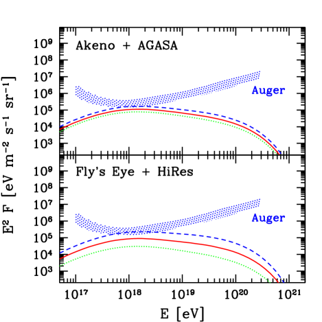
Figure 3: Left panel: Ultrahigh energy cosmic ray data with their statistical errors (top: combination of Akeno and AGASA data; bottom: combination of Fly’s Eye and HiRes data). The best fits between $E_{-}=10^{17.2}$ eV and $E_{+}=10^{20}$ eV, using the power-like injection spectrum, are given by the solid lines. The 2-sigma variations corresponding to the minimal (dotted) and maximal (dashed) fluxes are also shown. Other parameters of the analysis were $E_{\rm max}=3\times 10^{21}$ eV, $z_{\rm min}=0.012$, and $z_{\rm max}=2$. Right panel: Neutrino fluxes per flavour, $F_{\nu_{\ell}}+F_{\bar{\nu}_{\ell}}$, $\ell=e,\mu,\tau$. The “best” predictions for the neutrino spectra are given by the solid lines. The 2-sigma variations corresponding to the minimal (dotted) and maximal (dashed) fluxes are also shown.

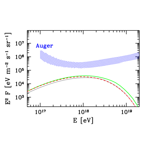
Figure 4: Lower bounds on the neutrino fluxes, $F_{\nu_{\ell}}+F_{\bar{\nu}_{\ell}}$, $\ell=e,\mu,\tau$, using a power-like proton injection spectrum, starting the fit at $E_{-}=10^{17.2}$ eV (dotted) or $E_{-}=10^{18.5}$ eV (dashed). In the latter case, $n$ is not constrained and we used $n=3$. Both are compatible with the lower bound obtained by the propagation inversion technique using $n=3$ (solid).

For larger $E_{\rm max}$, these confidence regions are unchanged. If we lower $E_{\rm max}$, they decrease and disappear at $E_{\rm max}=3\times 10^{20}$ eV for AGASA and $E_{\rm max}=1\times 10^{20}$ eV for HiRes, respectively. In order to get bounds on the cosmogenic neutrino flux, we vary $E_{\rm max}$, $\alpha$, and $n$, within their 2-sigma allowed values for both experiments. As there is still no consensus about the origin of UHECRs in the range from $10^{17}$ eV to $\approx 10^{19}$ eV, we perform the analyses using both $E_{-}=10^{17.2}$ eV and $E_{-}=10^{18.5}$ eV, respectively. The only difference, in the latter case, is that $n$ is no more constrained. As we will see in the next subsection, for a reasonable upper bound we have to assume that also the post-GZK events are protons from cosmological distances. This is clearly beyond the possibilities of a power-like injection spectrum. Therefore we conclude this subsection with a presentation of the inferred lower bound in Fig. 4.

3.2 Propagation inversion

The basic strategy of this subsection can be summarized as follows. Protons from cosmological distances contribute to the observed high energy cosmic rays (e.g. above $\approx 10^{18}$ eV). By means of the propagation function of the proton, one can determine the proton injection spectrum. This spectrum contains protons above the GZK cutoff, which results in cosmogenic neutrinos. Using a “minimal” or “maximal” proton contribution to the high energy cosmic rays, we can derive model-independent lower and upper bounds on the ultrahigh energy neutrino fluxes.

Usually, the propagation function is not invertible. A given detected spectrum $F_{b}(E)$ can be produced by several source luminosity distributions ${\mathcal{L}}_{p}(r,E_{i})$. As an illustration for this non-invertibility, one may think of two (unphysical) extreme cases. It could be that the whole detected spectrum is produced by nearby sources and no energy loss takes place. In this case the injection spectrum is the same as the observed one. In the other extreme case all the protons are produced at some large redshift $z_{\rm max}$. They lose their energy when they propagate through the universe and the injection spectrum contains much more high energy events than the observed one. Nevertheless, an unambiguous inversion can be carried out by fixing the $r$ dependence by some physical choice. We shall again assume an isotropic source luminosity distribution of the form (2), characterized by a redshift evolution parameter $n$ and $z_{\rm min/max}$.

From Eqs. (1) and (2), we find

$$F_{b}(E)=\int_{0}^{\infty}dE_{i}\ G_{b|p}(E,E_{i})\,J_{p}(E_{i}),$$ (6)

where $G_{b|p}(E,E_{i})$ is the space integral of Eq. (1). Instead of calculating the integral over $E_{i}$, usually one performs a summation over the energy bins,

$$F_{b}(E)=\sum_{E_{i}}\Delta E_{i}\ G_{b|p}(E,E_{i})\,J_{p}(E_{i})\,,\hskip 25.83325pt{\rm or}\hskip 25.83325pt{\bf F}_{b}={\bf G}_{b|p}\,{\bf J}_{p}\,,$$ (7)

where the second equation is the short-hand notation for the matrix-vector multiplication. With the help of ${\bf G}_{b|p}$, it is straightforward to invert the observed proton spectrum and to determine the resulting cosmogenic neutrino spectrum (in this case the particle type of “$b$” is “neutrino”),

$${\bf F}_{\nu}={\bf G}_{\nu|p}\,{\bf G}^{-1}_{p|p}\ {\bf F}_{p}\,,$$ (8)

where ${\bf F}_{p}$ is the vector notation of the observed proton flux $F_{p}(E)$.

The inversion procedure has an additional complication due to the fact that the observed spectrum in the high energy region has only a few events. The lack of large statistics results in significant statistical uncertainties. In order to take into account these effects, we used a Monte-Carlo and, for both experiments, we generated $10^{4}$ hypothetical observed spectra, compatible with the experimental results. Applying Eq. (8) to these spectra, one obtains the most probable cosmogenic neutrino flux, together with its statistical uncertainties.

Inverting these spectra, one obtains the most probable injection spectrum with its statistical uncertainties. Propagating these spectra through the universe, one infers a neutrino spectrum with its statistical uncertainties.

In order to enhance the different features of the observed spectrum, one usually multiplies it with the energy to some power, $E^{\gamma}$, where $\gamma=2\div 3$. In this “renormalized” spectrum, one observes an accumulation of events just around the GZK cutoff, as can be seen in Fig. 3 (left). A possible physical origin of this effect is apparent. Protons above the GZK cutoff lose their energy quite fast; however, as soon as they reach an energy around the GZK cutoff, their energy loss degrades very much. Thus, their relative number is larger. Other particles would produce such an enhancement at other energies and protons from nearby distances ($\raise 1.29167pt\hbox{$<$\kern-7.5pt\raise-4.73611pt\hbox{$\sim$}}\,50$ Mpc) would not produce such an enhancement at all. The apparent observation of this accumulation suggests, therefore, that the observed spectrum around the GZK cutoff is dominated by protons and that their sources are at cosmological distances. In our “minimal” scenario, only this part of the spectrum is assumed to be given by protons from cosmological distances. Since there are very good indications that this part of the spectrum is really a result of the GZK processes, the neutrinos, produced in the same processes, provide a robust lower bound on the cosmogenic neutrino flux. As a lower bound on the guaranteed cosmogenic part of the neutrino flux, it also serves as a robust lower bound on the total ultrahigh energy neutrino flux.

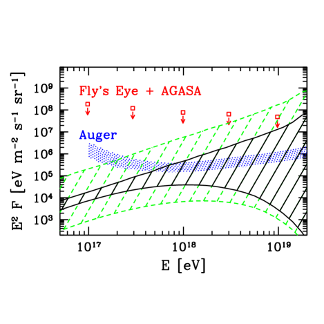
Figure 5: Bounds on the cosmogenic neutrino flux per flavour. Lower bounds use the fact that the accumulation in the normalized proton spectrum is a consequence of the GZK mechanism. Upper bounds assume that the whole spectrum, even the part above the GZK cutoff, originates from uniformly distributed proton sources with isotropic luminosity distribution. The region with the dashed boundary represents the maximal and minimal neutrino fluxes for which the cosmological evolution parameter was allowed to change between $0$ and $6$. The region with the solid boundary is obtained by a cosmological evolution parameter $n=3$. Boxes show the upper bounds obtained by combining Fly’s Eye [13] and Agasa [14] limits on deeply penetrating showers in different energy bins [15]. According to these limits, strong cosmological evolution ($n>3$) for the sources of the post-GZK events is already excluded.

There is no conventional astrophysical explanation for the observed comic rays events beyond the GZK cutoff. Even their particle composition is unknown. In our “maximal” scenario, we assume that they are all protons created isotropically in the universe. Thus, their injection spectrum was large enough to survive the GZK cutoff and produce the observed spectrum. Through the GZK mechanism, also these protons produce neutrinos. Since in this scenario we assume that all of the observed particles are protons (and calculate the associated cosmogenic neutrino flux), there is no more room for additional cosmogenic neutrinos. The bound we obtain is a robust upper bound on the cosmogenic neutrino flux (however, not necessarily an upper bound on the total neutrino flux).

In our inversion procedure, we used the observed cosmic ray spectrum between $E_{-}$ and $E_{+}$. We changed $E_{-}$ between $10^{17.0}$ eV and $10^{18.5}$ eV. Our results are rather insensitive to this choice.

In our “minimal” scenario, we obtained the lower bound on the neutrino flux. In order to check the sensitivity of our result on $E_{+}$, we lowered $E_{+}$ from $10^{20}$ eV to $10^{19.5}$ eV. The change of the neutrino fluxes is marginal for $E_{+}$ values between $10^{20}$ eV and $10^{19.8}$ eV. Taking an unphysically small value as low as $10^{19.5}$ eV, the change in the spectrum is smaller than the uncertainty of the expected sensitivity of the Auger experiment at $E_{+}=10^{18}$ eV (on the “renormalized” flux figure, the experiment is most sensitive at this energy, cf. Fig. 5). The GZK process suppresses the spectrum extremely effectively above $E\approx 10^{20}$ eV. Deviations from an expected GZK suppressed spectrum starts to be statistically significant above $E\approx 10^{20}$ eV. Therefore, we used $E_{+}=10^{20}$ eV in our analysis, similarly to our analysis based on a power-like proton injection flux. The lower bound for $n=3$ agrees well with the one obtained with the other technique (cf. Fig. 4).

In our “maximal” scenario, we used the whole observed spectrum up to the highest observed AGASA event in the $E=10^{20.4}$ eV energy-bin. In principle, there could be other neutrino sources than the GZK process, therefore the total neutrino flux might be even larger. However, since our maximal cosmogenic neutrino flux almost reaches the experimental limits (cf. Fig. 5), there is not much room for additional neutrinos. Note, that along with the cosmogenic neutrino flux there is also a cosmogenic photon flux from $\pi^{0}$ decay. After propagation, the photon flux associated with our upper bound in Fig. 5 may be in conflict with the EGRET observation of the diffuse gamma ray flux [32, 6]. For a detailed analysis, one would need the photon propagation functions [23] as well.

Our results on the neutrino flux bounds are summarized on Fig. 5. We used $n=3$ cosmological evolution. The variation due to the change of this parameter between $0$ and $6$ is also shown. Present [15] and expected [16] experimental bounds by AGASA, Fly’s Eye and Auger, respectively, are also presented.

4 Conclusions

In this Letter, we presented a systematic quantitative analysis of the minimal and maximal expected cosmogenic neutrino fluxes. The only assumption we made was that some part of the highest energy cosmic rays is due to protons from cosmological distances. We used two techniques. One of them assumed an $E_{i}^{-\alpha}$ power-like injection spectrum for the protons with some maximal cutoff energy $E_{\rm max}$. We compared the predicted spectrum after propagation with the observed one and determined the neutrino spectrum which was produced during the propagation. The second technique was based on an inversion of the observed proton flux around the GZK cutoff. The prediction for the lower bound on the cosmogenic neutrino fluxes were rather stable.

These lower bounds are of particular interest. They represent benchmarks for all neutrino telescopes and cosmic ray facilities designed to be sensitive in the ultrahigh energy region.

References

-
[1]
K. Greisen,
Phys. Rev. Lett. 16 (1966) 748;
G. T. Zatsepin and V. A. Kuzmin, JETP Lett. 4 (1966) 78 [Pisma Zh. Eksp. Teor. Fiz. 4 (1966) 114]. -
[2]
V. S. Berezinsky and G. T. Zatsepin,
Phys. Lett. B 28 (1969) 423;
V. S. Berezinsky and G. T. Zatsepin, Sov. J. Nucl. Phys. 11 (1970) 111 [Yad. Fiz. 11 (1970) 200]. -
[3]
F. W. Stecker,
Astrophys. J. 228 (1979) 919;
C. T. Hill and D. N. Schramm, Phys. Rev. D 31 (1985) 564;
C. T. Hill, D. N. Schramm and T. P. Walker, Phys. Rev. D 34 (1986) 1622;
F. W. Stecker, C. Done, M. H. Salamon and P. Sommers, Phys. Rev. Lett. 66 (1991) 2697 [Erratum-ibid. 69 (1991) 2738]. - [4] V. S. Berezinsky, in: Proc. DUMAND Summer Workshops, Learned, J.G. (Ed.), Khabarovsk and Lake Baikal, 22-31 Aug 1979, Hawaii DUMAND Center, University of Hawaii, 1980, pp. 245-261.
-
[5]
J. N. Bahcall and E. Waxman,
Phys. Rev. D 64 (2001) 023002;
E. Waxman and J. N. Bahcall, Phys. Rev. D 59 (1999) 023002. - [6] K. Mannheim, R. J. Protheroe and J. P. Rachen, Phys. Rev. D 63 (2001) 023003.
-
[7]
S. Yoshida and M. Teshima,
Prog. Theor. Phys. 89 (1993) 833;
S. Yoshida, H. y. Dai, C. C. Jui and P. Sommers, Astrophys. J. 479 (1997) 547. - [8] R. J. Protheroe and P. A. Johnson, Astropart. Phys. 4 (1996) 253 [Erratum-ibid. 5 (1996) 215].
- [9] R. Engel, D. Seckel and T. Stanev, Phys. Rev. D 64 (2001) 093010.
- [10] O. E. Kalashev, V. A. Kuzmin, D. V. Semikoz and G. Sigl, Phys. Rev. D 66 (2002) 063004.
- [11] Z. Fodor, S. D. Katz, A. Ringwald and H. Tu, Phys. Lett. B 561 (2003) 191.
- [12] H. Athar, M. Jezabek and O. Yasuda, Phys. Rev. D 62 (2000) 103007.
- [13] R. M. Baltrusaitis et al., Phys. Rev. D 31 (1985) 2192.
- [14] S. Yoshida et al. [AGASA Collaboration], in: Proc. 27th International Cosmic Ray Conference, Hamburg, Germany, 2001, Vol. 3, pp. 1142-1145.
- [15] L. A. Anchordoqui, J. L. Feng, H. Goldberg and A. D. Shapere, Phys. Rev. D 66 (2002) 103002.
-
[16]
X. Bertou, P. Billoir, O. Deligny, C. Lachaud and A. Letessier-Selvon,
Astropart. Phys. 17 (2002) 183;
C. Lachaud, X. Bertou, P. Billoir, O. Deligny and A. Letessier-Selvon, Nucl. Phys. Proc. Suppl. 110 (2002) 525. - [17] C. Spiering, J. Phys. G 29 (2003) 843.
- [18] V. S. Berezinsky and A. Y. Smirnov, Phys. Lett. B 48 (1974) 269.
-
[19]
D. A. Morris and A. Ringwald,
Astropart. Phys. 2 (1994) 43;
C. Tyler, A. V. Olinto and G. Sigl, Phys. Rev. D 63 (2001) 055001;
A. Ringwald and H. Tu, Phys. Lett. B 525 (2002) 135;
L. A. Anchordoqui, J. L. Feng, H. Goldberg and A. D. Shapere, Phys. Rev. D 65 (2002) 124027;
L. A. Anchordoqui, J. L. Feng, H. Goldberg and A. D. Shapere, hep-ph/0307228. - [20] J. N. Bahcall and E. Waxman, Astrophys. J. 542 (2000) 543.
- [21] Z. Fodor and S. D. Katz, Phys. Rev. D 63 (2001) 023002.
- [22] Z. Fodor, S. D. Katz and A. Ringwald, JHEP 0206 (2002) 046.
- [23] Z. Fodor, S. D. Katz and A. Ringwald, in preparation.
- [24] K. Hagiwara et al. [Particle Data Group Collaboration], Phys. Rev. D 66 (2002) 010001.
- [25] A. Mücke, R. Engel, J. P. Rachen, R. J. Protheroe and T. Stanev, Comput. Phys. Commun. 124 (2000) 290.
-
[26]
M. Takeda et al.,
Phys. Rev. Lett. 81 (1998) 1163;
http://www-akeno.icrr.u-tokyo.ac.jp/AGASA/ ; date: 24th February 2003. - [27] T. Abu-Zayyad et al. [HiRes Collaboration], astro-ph/0208243; astro-ph/0208301.
- [28] M. Nagano et al., J. Phys. G 18 (1992) 423.
-
[29]
D. J. Bird et al., Phys. Rev. Lett. 71 (1993) 3401;
D. J. Bird et al. [HIRES Collaboration], Astrophys. J. 424 (1994) 491;
D. J. Bird et al., Astrophys. J. 441 (1995) 144. - [30] M. Kachelriess, D. V. Semikoz and M. A. Tortola, hep-ph/0302161.
-
[31]
J. N. Bahcall and E. Waxman,
Phys. Lett. B 556 (2003) 1;
D. De Marco, P. Blasi and A. V. Olinto, Astropart. Phys. 20 (2003) 53. - [32] P. Sreekumar et al., Astrophys. J. 494 (1998) 523.