Abstract

We investigate the decays of $\pi^{0},\eta$ and $\eta^{\prime}$ into two photons in an effective $U(3)$ chiral Lagrangian approach without employing large $N_{c}$ arguments. Tree level and one-loop contributions from the anomalous Wess-Zumino-Witten Lagrangian are calculated and the importance of $\eta$-$\eta^{\prime}$ mixing is discussed. Unitarity corrections beyond one-loop play an important role for the decays with off-shell photons and are included by employing a coupled channel Bethe-Salpeter equation which satisfies unitarity constraints and generates vector-mesons from composed states of two pseudoscalar mesons.

PACS:	12.39.Fe, 13.40.Hq
Keywords:	Electromagnetic decays, chiral Lagrangians, unitarity,
	resonances.

1 Introduction

The two-photon decays $\pi^{0},\eta,\eta^{\prime}\rightarrow\gamma\gamma$ are phenomenological manifestations of the chiral anomaly of QCD and can provide important information on the chiral symmetry of the strong interactions. In order to study the phenomenological implications of the chiral anomaly, it is convenient to employ a chiral effective Lagrangian, since at low energies the effective degrees of freedom are colorless hadrons rather than quarks and gluons. The effective Lagrangian contains a piece which reproduces the anomalous behavior of the effective action under chiral transformations. Such a Lagrangian was systematically constructed by Wess and Zumino [1] by directly integrating the anomalous Ward identities and later Witten provided a representation of the anomaly which illustrated the topological content of the theory [2].

There are many anomalous processes which can be calculated from the Wess-Zumino-Witten (WZW) Lagrangian, such as $\pi^{0}\rightarrow\gamma\gamma,\eta\rightarrow\gamma\gamma,\gamma\rightarrow 3\pi,\eta\rightarrow\pi^{+}\pi^{-}\gamma$ etc. Originally, the WZW Lagrangian was formulated for the eight Goldstone bosons $(\pi,K,\eta)$ which form an octet under chiral $SU(3)$ transformations, but it can be easily extended to include the $\eta^{\prime}$, the singlet counterpart of the Goldstone boson octet [3, 4, 5, 6]. Although the $\eta^{\prime}$ is not a Goldstone boson due to the axial $U(1)$ anomaly of the strong interactions, it combines with the Goldstone bosons to a nonet at the level of the effective theory. This allows the phenomenological investigation of $\eta^{\prime}$ decays, such as $\eta^{\prime}\rightarrow\gamma\gamma$ and $\eta^{\prime}\rightarrow\pi^{+}\pi^{-}\gamma$.

The present work deals with the two-photon decays of $\pi^{0},\eta$ and $\eta^{\prime}$ with one, both or none of the photons being off-shell, $\pi^{0},\eta,\eta^{\prime}\rightarrow\gamma^{(*)}\gamma^{(*)}$. The decays $P\rightarrow\gamma\gamma\;(P=\pi^{0},\eta,\eta^{\prime})$ with both photons on-shell are dominated by the WZW Lagrangian. They have been calculated up to one-loop order within chiral perturbation theory (ChPT) and were shown not to receive non-analytic corrections from the one-loop diagrams which were compensated by the chiral corrections of the pseudoscalar decay constants [3, 4]. This is also in agreement with the complete one-loop renormalization of the anomalous Lagrangian [7, 8, 9], where it was shown by using heat kernel techniques that in dimensional regularization one-loop diagrams for $P\rightarrow\gamma\gamma$ do not lead to divergences that must be renormalized by appropriate counterterms of higher chiral order. It was furthermore argued [3] that a consistent picture of $\eta$-$\eta^{\prime}$ mixing emerged from the two-photon decays with one mixing angle of approximately $-20^{\circ}$.

More recently, a two-mixing angle scheme has been proposed by Kaiser and Leutwyler [5, 10, 11] for the calculation of the pseudoscalar decay constants in large $N_{c}$ chiral perturbation theory. The two angle scenario has been adopted in a phenomenological analysis of the two-photon decay widths of the $\eta$ and $\eta^{\prime}$, the $\eta\gamma$ and $\eta^{\prime}\gamma$ transition form factors, radiative $J/\Psi$ decays, as well as of the decay constants of the pseudoscalar mesons [12, 13]. The authors observe that within their phenomenological approach the assumption of one mixing angle is not in agreement with experiment whereas the two-mixing angle scheme leads to a very good description of the data. As pointed out in these investigations the analysis with two different mixing angles leads to a more coherent picture than the canonical treatment with a single angle. In particular, the calculation of the pseudoscalar decay constants within the framework of large $N_{c}$ chiral perturbation theory ${\it requires}$ two different mixing angles [10]. (A similar investigation was performed in [14] but with a different parameterization.)

In addition, it was shown in [15] that even at leading order $\eta$-$\eta^{\prime}$ mixing does not obey the usually assumed one-mixing-angle scheme, if large $N_{c}$ counting rules are not employed. One purpose of this work is to critically re-examine the contributions from $\eta$-$\eta^{\prime}$ mixing to the two-photon decays.

For the decays $P\rightarrow\gamma\gamma^{*}$ contributions from higher chiral orders will become increasingly more important for larger photon virtualities. In this case one-loop contributions turn out to be divergent and must be renormalized by appropriate counterterms [4, 7, 8]. The remaining finite parts of the relevant counterterms can be estimated by vector-meson exchange contributions [8]. In [8] the vector-mesons were included explicitly and integrating them out from the effective theory produced contact interactions. An underlying assumption of this approach is that the masses of the vector-mesons are much larger than the involved momenta.

Alternatively, the chiral Lagrangian for the Goldstone bosons is able to reproduce a number of meson resonances such as the $f_{0}$(980) and the $\rho$(770), when combined with non-perturbative Bethe-Salpeter approaches which are employed in such a way so that they ensure unitarity [16, 17]. Within these approaches effective coupled channel potentials are derived from the chiral meson Lagrangian and iterated in Bethe-Salpeter equations (BSEs). The BSE generates dynamically quasi-bound states of the mesons and accounts for the exchange of resonances without including them explicitly. The usefulness of this approach lies in the fact that from a small set of parameters a large variety of data can be explained and no additional assumptions need to be made on the couplings of the resonances. In [18] the approach has been extended to include the $\eta^{\prime}$ and successfully applied to the hadronic decays of $\eta$ and $\eta^{\prime}$ in [19]. The main purpose of the present work is to embed the coupled channel approach in the two-photon decays $P\rightarrow\gamma^{(*)}\gamma^{(*)}$ and to investigate the importance of vector-mesons for these decays from a different perspective. This will also allow us to give predictions for the double Dalitz decays with two off-shell photons which have not yet been studied experimentally. It may further clarify the question whether double vector-meson dominance holds, which is also an important issue for the anomalous magnetic moment of the muon and kaon decays [20].

This work is organized as follows. Section 2 introduces the notation and the tree level contributions to the decays which arise from the WZW Lagrangian. One-loop contributions and mixing effects are described and discussed in Sec. 3. The application of the coupled channel analysis to the decays is outlined in Sec. 4 and the numerical results are presented in Sec. 5. We conclude with a summary of our findings.

2 Decays at tree level

The effective Lagrangian for the pseudoscalar meson nonet ($\pi,K,\eta_{8},\eta_{0}$) reads up to second order in the derivative expansion [5, 11, 21, 22]

$$\mathcal{L}^{(0+2)} = -V_{0}+V_{1}\langle D_{\mu}U^{\dagger}D^{\mu}U\rangle+V_{2}\langle U^{\dagger}\chi+\chi^{\dagger}U\rangle+iV_{3}\langle U^{\dagger}\chi-\chi^{\dagger}U\rangle$$ (1)

$$\mathord{}+V_{4}\langle U^{\dagger}D^{\mu}U\rangle\langle U^{\dagger}D_{\mu}U\rangle$$

where we have presented only the terms relevant for the present work. The unitary matrix $U$ is a $3\times 3$ matrix containing the Goldstone boson octet ($\pi^{\pm},\tilde{\pi}^{0},K,\eta_{8}$) and the $\eta_{0}$. Its dependence on $\tilde{\pi}^{0},\eta_{8}$ and $\eta_{0}$ is given by

$$U=\exp\bigl{(}\mathrm{diag}(1,-1,0)\cdot i\tilde{\pi}^{0}/f+\mathrm{diag}(1,1,-2)\cdot i\eta_{8}/\sqrt{3}f+i\sqrt{2}\eta_{0}/\sqrt{3}f+\ldots\bigr{)}.$$ (2)

The expression $\langle\ldots\rangle$ denotes the trace in flavor space, $f$ is the pion decay constant in the chiral limit and the quark mass matrix $\mathcal{M}=\mbox{diag}(m_{u},m_{d},m_{s})$ enters in the combination $\chi=2B\mathcal{M}$ with $B=-\langle 0|\bar{q}q|0\rangle/f^{2}$ being the order parameter of the spontaneous symmetry violation. The covariant derivative is defined by

$$D_{\mu}U = \partial_{\mu}U-i(v_{\mu}+\tilde{a}_{\mu})U+iU(v_{\mu}-\tilde{a}_{\mu}).$$ (3)

The dependence of the effective Lagrangian on the running scale of QCD due to the anomalous dimension of the singlet axial current $A_{\mu}^{0}=\frac{1}{2}\bar{q}\gamma_{\mu}\gamma_{5}q$ is absorbed into the factor $\sqrt{\lambda}$ in the axial-vector connection $\tilde{a}_{\mu}$

$$\tilde{a}_{\mu}=a_{\mu}+\frac{\sqrt{6\lambda}-f}{3f}\langle a_{\mu}\rangle.$$ (4)

which is the scale independent combination of the octet and singlet parts of the external axial-vector field $a_{\mu}$, cf. [22] for details. Due to its scale dependence, $\sqrt{\lambda}$ cannot be determined from experiment, and all quantities involving it are unphysical.

The coefficients $V_{i}$ are functions of $\eta_{0}$, $V_{i}(\eta_{0}/f)$, and can be expanded in terms of this variable. At a given order of derivatives of the meson fields $U$ and insertions of the quark mass matrix $\mathcal{M}$ one obtains an infinite string of increasing powers of $\eta_{0}$ with couplings which are not fixed by chiral symmetry. Parity conservation implies that the $V_{i}$ are all even functions of $\eta_{0}$ except $V_{3}$, which is odd, and $V_{1}(0)=V_{2}(0)=V_{1}(0)-3V_{4}(0)=\frac{1}{4}f^{2}$ gives the correct normalization for the quadratic terms of the mesons. The potentials $V_{i}$ are expanded in the singlet field $\eta_{0}$

$$V_{i}\Big{[}\frac{\eta_{0}}{f}\Big{]} = v_{i}^{(0)}+v_{i}^{(2)}\frac{\eta_{0}^{2}}{f^{2}}+v_{i}^{(4)}\frac{\eta_{0}^{4}}{f^{4}}+\ldots\qquad\mbox{for}\quad i=0,1,2,4$$

$$V_{3}\Big{[}\frac{\eta_{0}}{f}\Big{]} = v_{3}^{(1)}\frac{\eta_{0}}{f}+v_{3}^{(3)}\frac{\eta_{0}^{3}}{f^{3}}+\ldots\quad$$ (5)

with expansion coefficients $v_{i}^{(j)}$ to be determined phenomenologically.

The Lagrangian $\mathcal{L}^{(0+2)}$ contains only terms of natural parity. The photonic decays $\pi\rightarrow\gamma\gamma,\eta\rightarrow\gamma\gamma,\eta^{\prime}\rightarrow\gamma\gamma$, on the other hand, are not covered by $\mathcal{L}^{(0+2)}$, since they arise from the unnatural parity part of the effective Lagrangian which collects the terms that are proportional to the tensor $\epsilon_{\mu\nu\alpha\beta}$. Within the effective theory the chiral anomalies of the underlying QCD Lagrangian are accounted for by the WZW term [1, 2, 5]

$$S_{\scriptscriptstyle{WZW}}(U,v)=\int d^{4}x\mathcal{L}_{\scriptscriptstyle{WZW}}=-\frac{i}{80\pi^{2}}\int_{M_{5}}\langle\Sigma^{5}\rangle-\frac{i}{16\pi^{2}}\int_{M_{4}}W(U,v)$$ (6)

where

$$W(U,v)=\langle\Sigma U^{\dagger}dvUv+\Sigma vdv+\Sigma dvv-i\Sigma^{3}v\rangle-(U\leftrightarrow U^{\dagger})$$ (7)

with $\Sigma=U^{\dagger}dU$ and we set $N_{c}=3$ for the number of colors. We have displayed only the pieces of the Lagrangian relevant for the present work and adopted the differential form notation of [5]

$$v=dx^{\mu}v_{\mu},\qquad d=dx^{\mu}\partial_{\mu}$$ (8)

with the Grassmann variables $dx^{\mu}$ which yield the volume element $dx^{\mu}dx^{\nu}dx^{\alpha}dx^{\beta}=\epsilon^{\mu\nu\alpha\beta}d^{4}x$. The operation $(U\leftrightarrow U^{\dagger})$ indicates the interchange of $U$ and $U^{\dagger}$. The first integral on the right-hand side in Eq. (6) is taken over the five-dimensional manifold $M_{5}$ which is the direct product of the Minkowski space $M_{4}$ and the finite interval $0\leq x^{5}\leq 1$, while the Grassmann algebra is supplemented by the fifth element $dx^{5}$. The matrix-valued fields $U(x,x^{5})$ in the first integral are functions on this five-dimensional manifold and interpolate smoothly between the identity matrix $U(x,0)=\mathds{1}$ and the matrix $U(x)=U(x,1)$. The value of the first integral is independent on the particular choice of the interpolating functions $U(x,x^{5})$, whereas the integration for the second term in Eq. (6) extends only over the Minkowski space $M_{4}$. The external vector field $v=-eQA$ describes the coupling of the photon field $A=dx^{\mu}A_{\mu}$ to the mesons with $Q=\frac{1}{3}\mbox{diag}(2,-1,-1)$ being the charge matrix of the light quarks.

At tree level only the terms quadratic in the vector fields $v$ contribute and one arrives at the following pieces of the WZW Lagrangian

$$d^{4}x\mathcal{L}_{\scriptscriptstyle{WZW}} = -\frac{i}{16\pi^{2}}\langle U^{\dagger}dUU^{\dagger}dvUv+U^{\dagger}dUvdv+U^{\dagger}dUdvv$$ (9)

$$\qquad\quad-UdU^{\dagger}UdvU^{\dagger}v-UdU^{\dagger}vdv-UdU^{\dagger}dvv\rangle+\ldots\;.$$

However, this is not the whole story, since there exist further terms at fourth chiral order which are gauge invariant and do not contribute to the chiral anomalies. A complete set of these terms has been given in [5], out of which the following three contact terms contribute

$$d^{4}x\mathcal{L}_{\scriptscriptstyle{ct}}^{(4)}=W_{1}\langle UdvU^{\dagger}dv\rangle+W_{2}\langle dvdv\rangle+iW_{3}\langle dUdU^{\dagger}dv+dU^{\dagger}dUdv\rangle,$$ (10)

where the potentials $W_{1,2,3}$ are odd functions of the singlet field $\eta_{0}$. The first two terms contribute already at tree level, whereas the last term represents a vertex for a one-loop diagram and will be discussed in the next section. Following the steps of [22] it is straightforward to see that these terms are needed to absorb the QCD renormalization scale dependence via a set of redefinitions of the potentials $W_{i}$ into the factor $\sqrt{\lambda}$ of $\tilde{a}_{\mu}$ in Eq. (4).

The decay at tree level is depicted in Figure 1

Figure 1: Tree diagram of the decay $P\to\gamma^{(*)}\gamma^{(*)}$, where $k^{(\prime)}$ and $\epsilon^{(\prime)}$ denote the momenta and polarizations of the photons, respectively.

and the pertinent amplitudes are given by

$$\mathcal{A}^{\textit{(tree)}}(P\rightarrow\gamma^{(*)}\gamma^{(*)})=e^{2}k_{\mu}\epsilon_{\nu}k^{\prime}_{\alpha}\epsilon^{\prime}_{\beta}\epsilon^{\mu\nu\alpha\beta}\frac{1}{4\pi^{2}f}\alpha_{P}^{\textit{(tree)}}$$ (11)

with

$$\alpha_{\pi^{0}}^{\textit{(tree)}}=1,\qquad\qquad\alpha_{\eta}^{\textit{(tree)}}=\frac{1}{\sqrt{3}},\qquad\qquad\alpha_{\eta^{\prime}}^{\textit{(tree)}}=2\sqrt{\frac{2}{3}}-\frac{16\pi^{2}}{3}(w_{1}^{(1)}+w_{2}^{(1)}),$$ (12)

where $w_{1}^{(1)}$, $w_{2}^{(1)}$ are the leading expansion coefficients of the potentials $W_{1}$ and $W_{2}$, respectively. It is important to note that in our scheme $\eta$-$\eta^{\prime}$ mixing is of second chiral order [15] and will modify the sub-leading order, i.e. the one-loop order of the decay amplitudes. This is in contradistinction to large $N_{c}$ ChPT where $\eta$-$\eta^{\prime}$ mixing contributes at leading order.

3 One-loop contributions

The one-loop diagrams for $P\rightarrow\gamma^{(*)}\gamma^{(*)}$ of order $\mathcal{O}(p^{6})$ have anomalous vertices from the following pieces of the WZW Lagrangian

$$d^{4}x\mathcal{L}_{\scriptscriptstyle{WZW}} = -\frac{i}{16\pi^{2}}\langle U^{\dagger}dUU^{\dagger}dvUv+U^{\dagger}dUvdv+U^{\dagger}dUdvv-iU^{\dagger}dUU^{\dagger}dUU^{\dagger}dUv\rangle$$ (13)

$$-(U\leftrightarrow U^{\dagger})+\ldots\;.$$

After expanding $U=\exp(\frac{i\sqrt{2}}{f}\phi)$ in the meson fields $\phi$ we arrive at the expression

$$d^{4}x\mathcal{L}_{\scriptscriptstyle{WZW}}=-\frac{\sqrt{2}}{8\pi^{2}f^{3}}\Big{(}\langle d\phi\,[\phi,[\phi\,,v\,dv\,]]\rangle-\langle d\phi\,[\phi\,,dv]\,[\phi,\,v]\rangle-2i\langle d\phi\,d\phi\,d\phi\,v\rangle\Big{)}+\ldots\;,$$ (14)

where we have only presented the relevant terms for the one-loop diagrams. The one-loop diagrams at order $\mathcal{O}(p^{6})$ contributing to the decays $P\rightarrow\gamma^{(*)}\gamma^{(*)}$ are shown in Fig. 2.

(a)

(b)

Figure 2: One-loop diagrams contributing to $P\to\gamma^{(*)}\gamma^{(*)}$. In (b) the crossed diagram is not shown.

The tadpole contributions in Fig. 2a read

$$\mathcal{A}^{\textit{(tad)}}(P\rightarrow\gamma^{(*)}\gamma^{(*)})=e^{2}k_{\mu}\epsilon_{\nu}k^{\prime}_{\alpha}\epsilon^{\prime}_{\beta}\epsilon^{\mu\nu\alpha\beta}\frac{1}{4\pi^{2}F_{P}^{3}}\Big{(}\beta_{P}^{\textit{(tad)},\pi}\Delta_{\pi}+\beta_{P}^{\textit{(tad)},K}\Delta_{K}\Big{)}$$ (15)

with $\Delta_{\phi}$ being the finite parts of the tadpoles

$$\Delta_{\phi}=\left(\int\frac{d^{d}l}{(2\pi)^{d}}\frac{i}{l^{2}-m_{\phi}^{2}+i\epsilon}\right)_{\textit{finite}}=\frac{m_{\phi}^{2}}{16\pi^{2}}\,\ln\frac{m_{\phi}^{2}}{\mu^{2}},$$ (16)

and $\mu$ is the scale introduced in dimensional regularization. In the present work we are only concerned with the finite pieces of the diagrams and neglect the divergent portions throughout. The coefficients $\beta_{P}^{\textit{(tad)},\phi}$ are given by

$$\begin{array}[]{lcllcllcl}\beta_{\pi}^{\textit{(tad)},\pi}&=&-\dfrac{4}{3},&\beta_{\eta}^{\textit{(tad)},\pi}&=&-\dfrac{2}{\sqrt{3}},&\beta_{\eta^{\prime}}^{\textit{(tad)},\pi}&=&-2\sqrt{\dfrac{2}{3}}+16\pi^{2}w_{1}^{(1)},\\ \beta_{\pi}^{\textit{(tad)},K}&=&-\dfrac{5}{3},&\beta_{\eta}^{\textit{(tad)},K}&=&-\dfrac{1}{\sqrt{3}},&\beta_{\eta^{\prime}}^{\textit{(tad)},K}&=&-2\sqrt{\dfrac{2}{3}}+16\pi^{2}w_{1}^{(1)}.\end{array}$$ (17)

We have furthermore replaced the pion decay constant in the chiral limit, $f$, by the expressions $F_{P}$ which include the one-loop corrections. The corrections have been calculated in $U(3)$ ChPT without imposing large $N_{c}$ counting rules and in infrared regularization [15]. We can employ the same formulae also for the present work by noting that only tadpoles contribute at one-loop order to the decay constants. In infrared regularization the $\eta^{\prime}$ tadpole vanishes, whereas the tadpoles for the Goldstone boson octet remain unaltered. This implies that the $\eta^{\prime}$ tadpole does not contain any infrared physics and can be absorbed completely into the low-energy constants (LECs) of the effective Lagrangian. It is neither a function of the Goldstone boson masses nor of the external momenta, it is just a constant. We will therefore assume that $\eta^{\prime}$ tadpole contributions have been compensated by renormalizing the LECs appropriately and will work with the renormalized values without indicating it explicitly.

The expansions of the decay constants in terms of the Goldstone boson masses up to one-loop order are given here for completeness [15]

$$F_{\pi} = f\Big{[}1+4\beta_{4}^{(0)}\frac{2m_{K}^{2}+m_{\pi}^{2}}{f^{2}}+4\beta_{5}^{(0)}\frac{m_{\pi}^{2}}{f^{2}}-\frac{\Delta_{\pi}+{\textstyle\frac{1}{2}}\Delta_{K}}{f^{2}}\Big{]},$$

$$F_{\eta} = f\Big{[}1+4\beta_{4}^{(0)}\frac{2m_{K}^{2}+m_{\pi}^{2}}{f^{2}}+4\beta_{5}^{(0)}\frac{m_{\eta}^{2}}{f^{2}}-\frac{{\textstyle\frac{3}{2}}\Delta_{K}}{f^{2}}\Big{]},$$

$$F_{\eta^{\prime}} = \frac{f}{\sqrt{6\lambda}}F_{\eta^{\prime}0}=f\Big{[}1+4\frac{2m_{K}^{2}+m_{\pi}^{2}}{3f^{2}}\big{(}3\beta_{4}^{(0)}+\beta_{5}^{(0)}-9\beta_{17}^{(0)}+3\beta_{18}^{(0)}$$ (18)

$$\qquad\qquad\qquad\qquad\qquad\qquad\mathrel{}+3\beta_{46}^{(0)}+9\beta_{47}^{(0)}-3\beta_{53}^{(0)}-\frac{3}{2}\sqrt{6}\beta_{52}^{(1)}\big{)}\Big{]}.$$

The LECs $\beta_{i}^{(j)}$ originate from the natural parity part of the effective Lagrangian at fourth chiral order

$$\mathcal{L}^{(4)}=\mathop{\textstyle\sum}\nolimits_{k}\beta_{k}O_{k},$$ (19)

where the contributing fourth order operators are

$$\begin{array}[]{ll}O_{\phantom{0}4}=-\langle C^{\mu}C_{\mu}\rangle\langle M\rangle,&O_{\phantom{0}5}=-\langle C^{\mu}C_{\mu}M\rangle,\\ O_{17}=\langle C^{\mu}\rangle\langle C_{\mu}\rangle\langle M\rangle,&O_{18}=-\langle C^{\mu}\rangle\langle C_{\mu}M\rangle,\\ O_{46}=2i\langle\tilde{a}_{\mu}\rangle\langle C^{\mu}M\rangle,&O_{47}=2i\langle\tilde{a}_{\mu}\rangle\langle C^{\mu}\rangle\langle M\rangle,\\ O_{52}=-2\langle M\rangle\partial^{\mu}\langle\tilde{a}_{\mu}\rangle,&O_{53}=2i\langle N\rangle\partial^{\mu}\langle\tilde{a}_{\mu}\rangle,\end{array}$$ (20)

and we made use of the following abbreviations

$$C_{\mu}=U^{\dagger}D_{\mu}U,\qquad\qquad M=U^{\dagger}\chi+\chi^{\dagger}U,\qquad\qquad N=U^{\dagger}\chi-\chi^{\dagger}U.$$ (21)

The $\beta_{k}$ are functions of the singlet field, $\beta_{k}(\eta_{0})$, and can be expanded in the same manner as the $V_{i}(\eta_{0})$. Note that the $\beta_{k}$ also have divergent pieces, in order to compensate the divergences from the loops, but in the present work we are only concerned with the finite parts and use the same notation for simplicity. The decay constant of the $\eta^{\prime}$ related to the singlet axial-vector current, $F_{\eta^{\prime}0}$, is defined by the matrix element

$$\langle 0|{\textstyle\frac{1}{\sqrt{6}}}\bar{q}\gamma_{\mu}\gamma_{5}q|\eta^{\prime}\rangle=ip_{\mu}F_{\eta^{\prime}0}.$$ (22)

Due to the anomalous dimension of the singlet axial current, $F_{\eta^{\prime}0}$ depends on the running scale of QCD and its value cannot be determined phenomenologically. In order to account for the chiral corrections for $f$, we have therefore employed the scale invariant ratio $F_{\eta^{\prime}}=\frac{f}{\sqrt{6\lambda}}F_{\eta^{\prime}0}$ in the expression for the $\eta^{\prime}$ decay amplitude in Eq. (15).

We replace the pion decay constant in the chiral limit, $f$, by the chirally corrected decay constants $F_{P}$ also in the tree level result, Eq. (11). This replacement yields corrections at $\mathcal{O}(p^{6})$ which must be compensated. If the decay constants $F_{P}$ in Eq. (3) are written as $F_{P}=f(1+\delta F_{P}/f^{2})$, it induces at sixth chiral order the corrections

$$\mathcal{A}^{(f)}(P\rightarrow\gamma^{(*)}\gamma^{(*)})=e^{2}k_{\mu}\epsilon_{\nu}k^{\prime}_{\alpha}\epsilon^{\prime}_{\beta}\epsilon^{\mu\nu\alpha\beta}\frac{1}{4\pi^{2}F_{P}^{3}}\alpha_{P}^{\textit{(tree)}}\delta F_{P}.$$ (23)

The contributions from diagram 2b yield

$$\mathcal{A}^{\textit{(uni)}}(P\rightarrow\gamma^{(*)}\gamma^{(*)}) = e^{2}k_{\mu}\epsilon_{\nu}k^{\prime}_{\alpha}\epsilon^{\prime}_{\beta}\epsilon^{\mu\nu\alpha\beta}\frac{1}{4\pi^{2}F_{P}^{3}}\Big{(}\beta_{P}^{\textit{(uni)},\pi}[I(m_{\pi}^{2};k^{2})+I(m_{\pi}^{2};k^{\prime 2})]$$ (24)

$$\qquad\qquad\qquad\qquad+\beta_{P}^{\textit{(uni)},K}[I(m_{K}^{2};k^{2})+I(m_{K}^{2};k^{\prime 2})]\Big{)}.$$

The integral $I$ is given by

$$I(m^{2};p^{2})=\frac{2}{3}\Big{(}\frac{1}{2}\Delta+(m^{2}-\frac{p^{2}}{4})G_{mm}(p^{2})+\frac{1}{96\pi^{2}}(p^{2}-6m^{2})\Big{)},$$ (25)

where $G$ is the finite part of the scalar one-loop integral

$$G_{m\bar{m}}(p^{2})=\mathrel{}\left(\int\frac{\,d^{d}l}{(2\pi)^{d}}\,\frac{i}{(l^{2}-m^{2}+i\epsilon)((l-p)^{2}-\bar{m}^{2}+i\epsilon)}\right)_{\textit{finite}}$$ (26)

which reads

$$G_{m\bar{m}}(p^{2})= \mathrel{}\frac{1}{16\pi^{2}}\bigg{[}-1+\ln\frac{m\bar{m}}{\mu^{2}}+\frac{m^{2}-\bar{m}^{2}}{p^{2}}\ln\frac{m}{\bar{m}}$$

$$\qquad\qquad\quad\mathord{}-\frac{2\sqrt{\lambda_{m\bar{m}}(p^{2})}}{p^{2}}\mathop{\mathrm{artanh}}\nolimits\frac{\sqrt{\lambda_{m\bar{m}}(p^{2})}}{(m+\bar{m})^{2}-p^{2}}\bigg{]},$$

$$\lambda_{m\bar{m}}(p^{2})= \mathrel{}\big{(}(m-\bar{m})^{2}-p^{2}\big{)}\big{(}(m+\bar{m})^{2}-p^{2}\big{)}.$$ (27)

For the particular case with on-shell photons the integral $I$ reduces to the simple expression $I(m^{2};0)=\Delta$. The coefficients $\beta_{P}^{\textit{(uni)},\phi}$ are given by

$$\begin{array}[]{lcllcllcl}\beta_{\pi}^{\textit{(uni)},\pi}&=&1,&\beta_{\eta}^{\textit{(uni)},\pi}&=&\dfrac{1}{\sqrt{3}},&\beta_{\eta^{\prime}}^{\textit{(uni)},\pi}&=&\sqrt{\dfrac{2}{3}}-16\pi^{2}w_{3}^{(1)},\\ \beta_{\pi}^{\textit{(uni)},K}&=&1,&\beta_{\eta}^{\textit{(uni)},K}&=&\dfrac{1}{\sqrt{3}},&\beta_{\eta^{\prime}}^{\textit{(uni)},K}&=&\sqrt{\dfrac{2}{3}}-16\pi^{2}w_{3}^{(1)}.\end{array}$$ (28)

3.1 Wave-function renormalization, $\eta$-$\eta^{\prime}$ mixing, and counterterms

There are further chiral corrections at $\mathcal{O}(p^{6})$ which arise from wave-function renormalization and $\eta$-$\eta^{\prime}$ mixing. The relation between the original $SU(3)$ fields ($\tilde{\pi}^{0},\eta_{8},\eta_{0}$) and the renormalized states ($\pi^{0},\eta,\eta^{\prime}$) without employing large $N_{c}$ counting rules has already been derived in [15]. It is given in terms of the $3\times 3$ matrix $\mathds{1}+R^{(2)}$, $(\tilde{\pi}^{0},\eta_{8},\eta_{0})^{T}=(\mathds{1}+R^{(2)})(\pi^{0},\eta,\eta^{\prime})^{T}$, with

$$R^{(2)}_{\tilde{\pi}^{0}\pi^{0}} = \bigl{(}-4[2m_{K}^{2}+m_{\pi}^{2}]\beta_{4}^{(0)}-4m^{2}_{\pi}\beta_{5}^{(0)}+{\textstyle\frac{1}{3}}\Delta_{\pi}+{\textstyle\frac{1}{6}}\Delta_{K}\bigr{)}/F_{\pi}^{2},$$

$$R^{(2)}_{8\eta} = \bigl{(}-4[2m_{K}^{2}+m_{\pi}^{2}]\beta_{4}^{(0)}-4m_{\eta}^{2}\beta_{5}^{(0)}+{\textstyle\frac{1}{2}}\Delta_{K}\bigr{)}/F_{\eta}^{2},$$

$$R^{(2)}_{8\eta^{\prime}} = \frac{8\sqrt{2}}{3}(m_{K}^{2}-m_{\pi}^{2})\bigl{(}2{\overset{\circ}{m}\vphantom{m}_{0}^{2}}\beta_{5,18}-\tilde{v}_{2}^{(1)}\bigr{)}\big{/}F_{\eta^{\prime}}^{2}{\overset{\circ}{m}\vphantom{m}_{0}^{2}},$$

$$R^{(2)}_{0\eta} = \frac{8\sqrt{2}}{3}(m_{K}^{2}-m_{\pi}^{2})\tilde{v}_{2}^{(1)}\big{/}F_{\eta}^{2}{\overset{\circ}{m}\vphantom{m}_{0}^{2}},$$

$$R^{(2)}_{0\eta^{\prime}} = -\frac{4}{3}(2m_{K}^{2}+m_{\pi}^{2})(3\beta_{4}^{(0)}+\beta_{5}^{(0)}-9\beta_{17}^{(0)}+3\beta_{18}^{(0)})/F_{\eta^{\prime}}^{2},$$ (29)

and all remaining entries vanish . In Eq. (3.1) we have used the abbreviations

$${\overset{\circ}{m}\vphantom{m}_{0}^{2}} = \frac{2v_{0}^{(2)}}{f^{2}},$$

$$\tilde{v}_{2}^{(1)} = {\textstyle\frac{1}{4}}f^{2}-{\textstyle\frac{1}{2}}\sqrt{6}v_{3}^{(1)},$$

$$\beta_{5,18} = \beta_{5}^{(0)}+{\textstyle\frac{3}{2}}\beta_{18}^{(0)}.$$ (30)

Within this scenario, $\eta$-$\eta^{\prime}$ mixing contributes at next-to-leading order which is in contradistinction to large $N_{c}$ ChPT [23], where it is a leading order effect. Inserting these relations into the tree level result Eq. (11) one obtains the following corrections at sixth chiral order

$$\mathcal{A}^{(Z)}(P\rightarrow\gamma^{(*)}\gamma^{(*)})=e^{2}k_{\mu}\epsilon_{\nu}k^{\prime}_{\alpha}\epsilon^{\prime}_{\beta}\epsilon^{\mu\nu\alpha\beta}\frac{1}{4\pi^{2}F_{P}}\beta^{(Z)}_{P}$$ (31)

with the coefficients

$$\beta^{(Z)}_{\pi^{0}} = \alpha_{\pi^{0}}^{\textit{(tree)}}R^{(2)}_{\tilde{\pi}^{0}\pi^{0}}$$

$$\beta^{(Z)}_{\eta} = \alpha_{\eta}^{\textit{(tree)}}R^{(2)}_{8\eta}+\alpha_{\eta^{\prime}}^{\textit{(tree)}}R^{(2)}_{0\eta}$$

$$\beta^{(Z)}_{\eta^{\prime}} = \alpha_{\eta}^{\textit{(tree)}}R^{(2)}_{8\eta^{\prime}}+\alpha_{\eta^{\prime}}^{\textit{(tree)}}R^{(2)}_{0\eta^{\prime}}.$$ (32)

Summing all the contributions at order $\mathcal{O}(p^{6})$ we verify that for the $\pi^{0}$- and $\eta$-decays into two on-shell photons the dependence on the regularization scale $\mu$ cancels out, i.e. the amplitudes are finite and do not need to be renormalized by counterterms of the unnatural parity part of the $p^{6}$ Lagrangian [3, 4, 7, 8]. For the process $\eta^{\prime}\to\gamma\gamma$, to the contrary, the $w_{3}^{(1)}$ term of the unnatural parity Lagrangian at fourth chiral order induces a non-vanishing $\mu$ dependence via a loop. Also, for the decays with one or both photons off-shell the divergent parts do not cancel for any of the decaying mesons and again a residual scale dependence remains which can be compensated by introducing counterterms at sixth order. The explicit renormalization of the amplitudes which are induced by the WZW term has been accomplished in [7, 8] and is beyond the scope of the present investigation, where we restrict ourselves to the finite pieces of the integrals and counterterms.

In the $SU(3)$ framework without an explicit $\eta^{\prime}$, the Lagrangian of unnatural parity at $\mathcal{O}(p^{6})$ has been constructed in [24]. The relevant terms contributing via tree diagrams to the decays are presented in App. A, where we also show an additional set of counterterms which arises due to the extension to the $U(3)$ framework. These terms can be reduced to the following structures (restricting ourselves to the finite pieces of the coupling constants)

$$\begin{array}[]{lcclccl}\mathcal{L}_{ct}^{(6)}&=&-&\bar{w}_{1}^{(0)}\ \frac{16\sqrt{2}}{f}\ \langle\phi\ dv\ \square\,dv\rangle&+&\bar{w}_{2}^{(1)}\ \frac{16}{f}\ \eta_{0}\ \langle dv\ \square\,dv\rangle\\ &&+&\bar{w}_{3}^{(0)}\ \frac{32\sqrt{2}}{f}\langle\phi\,\chi\,dv\,dv\rangle&+&\bar{w}_{4}^{(0)}\ \frac{32\sqrt{2}}{f}\langle\phi\,\chi\rangle\langle dv\,dv\rangle\\ &&+&\bar{w}_{5}^{(1)}\,\ \frac{32}{f}\ \eta_{0}\langle\chi\,dv\,dv\rangle&+&\bar{w}_{6}^{(1)}\,\ \frac{32}{f}\ \eta_{0}\langle\chi\rangle\langle dv\,dv\rangle,\end{array}$$ (33)

where we employed the LECs of the original counterterms in App. A. Note that the first two terms only contribute to the decays with off-shell photons. The contribution of $\mathcal{L}_{ct}^{(6)}$ to the decays reads

$$\mathcal{A}^{\textit{(ct)}}=(P\rightarrow\gamma^{(*)}\gamma^{(*)})=e^{2}k_{\mu}\epsilon_{\nu}k^{\prime}_{\alpha}\epsilon^{\prime}_{\beta}\epsilon^{\mu\nu\alpha\beta}\frac{1}{4\pi^{2}F_{P}}\beta^{(ct)}_{P}$$ (34)

with the coefficients

$$\beta^{(ct)}_{\pi^{0}} = -\frac{64}{3}\pi^{2}[(k^{2}+{k^{\prime}}^{2})\bar{w}_{1}^{(0)}+4m_{\pi}^{2}\bar{w}_{3}^{(0)}],$$

$$\beta^{(ct)}_{\eta} = -\frac{64}{3\sqrt{3}}\pi^{2}\left[(k^{2}+{k^{\prime}}^{2})\bar{w}_{1}^{(0)}-\frac{4}{3}(4m_{K}^{2}-7m_{\pi}^{2})\bar{w}_{3}^{(0)}-32(m_{K}^{2}-m_{\pi}^{2})\bar{w}_{4}^{(0)}\right],$$

$$\beta^{(ct)}_{\eta^{\prime}} = -\frac{128}{3}\pi^{2}\left[(k^{2}+{k^{\prime}}^{2})(\sqrt{\frac{2}{3}}\bar{w}_{1}^{(0)}-\bar{w}_{2}^{(1)})+\frac{4}{3}(m_{K}^{2}+2m_{\pi}^{2})(\sqrt{\frac{2}{3}}\bar{w}_{3}^{(0)}+\bar{w}_{5}^{(1)})\right.$$ (35)

$$\qquad\qquad\left.+4(2m_{K}^{2}+m_{\pi}^{2})(\sqrt{\frac{2}{3}}\bar{w}_{4}^{(0)}+\bar{w}_{6}^{(1)})\right].$$

3.2 Numerical results at one-loop order

Before implementing the unitarity corrections beyond one-loop within the Bethe Salpeter approach, we would like to extract numerical results from the one-loop expressions for the decays into two physical photons, $P\rightarrow\gamma\gamma$. Combining all the contributions of the preceding sections we arrive at

$$\mathcal{A}^{\textit{(1-loop)}}=\mathcal{A}^{\textit{(tree)}}+\mathcal{A}^{\textit{(tad)}}+\mathcal{A}^{\textit{(uni)}}+\mathcal{A}^{(f)}+\mathcal{A}^{(Z)}+\mathcal{A}^{(ct)}.$$ (36)

The decay width $\Gamma$ is given by

$$\Gamma(P\rightarrow\gamma\gamma)=\frac{\alpha^{2}m_{P}^{3}}{64\pi^{3}F_{P}^{2}}\;|\,\beta_{P}^{\textit{(1-loop)}}\,|^{\,2}$$ (37)

with $\alpha=e^{2}/4\pi$ and

$$\beta_{P}^{\textit{(1-loop)}}=\alpha_{P}^{\textit{(tree)}}\left(1+\frac{\delta F_{P}}{F_{P}^{2}}\right)+(\beta_{P}^{\textit{(tad)},\pi}+2\beta_{P}^{\textit{(uni)},\pi})\frac{\Delta_{\pi}}{F_{P}^{2}}+(\beta_{P}^{\textit{(tad)},K}+2\beta_{P}^{\textit{(uni)},K})\frac{\Delta_{K}}{F_{P}^{2}}+\beta_{P}^{(Z)}+\beta_{P}^{(ct)}.$$ (38)

For comparison with previous work [3, 4] we also present the explicit form of the $\beta_{P}^{\textit{(1-loop)}}$ coefficients

$$\beta_{\pi^{0}}^{\textit{(1-loop)}} = 1-\frac{256\pi^{2}}{3}m_{\pi}^{2}\bar{w}_{3}^{(0)},$$

$$\beta_{\eta}^{\textit{(1-loop)}} = \frac{1}{\sqrt{3}}\left\{1+\frac{1}{F_{\eta}^{2}}\frac{32}{3}\left[1-\sqrt{\frac{2}{3}}\ 4\pi^{2}(w_{1}^{(1)}+w_{2}^{(1)})\right](m_{K}^{2}-m_{\pi}^{2})\frac{\tilde{v}_{2}^{(1)}}{{\overset{\circ}{m}\vphantom{m}_{0}^{2}}}\right.$$

$$\qquad\left.+\ \frac{256}{9}\pi^{2}\ [(4m_{K}^{2}-7m_{\pi}^{2})\bar{w}_{3}^{(0)}+24(m_{K}^{2}-m_{\pi}^{2})\bar{w}_{4}^{(0)}]\right\},$$

$$\beta_{\eta^{\prime}}^{\textit{(1-loop)}} = \left[2\sqrt{\frac{2}{3}}-\frac{16\pi^{2}}{3}(w_{1}^{(1)}+w_{2}^{(1)})\right]\left\{1+\frac{1}{F_{\eta^{\prime}}^{2}}\left[4(2m_{K}^{2}+m_{\pi}^{2})(\beta_{46}^{(0)}+3\beta_{47}^{(0)}-\beta_{53}^{(0)}-\sqrt{\frac{3}{2}}\beta_{52}^{(1)})\right]\right\}$$ (39)

$$\qquad+\ \frac{1}{F_{\eta^{\prime}}^{2}}\left[16\pi^{2}(w_{1}^{(1)}-2w_{3}^{(1)})(\Delta_{\pi}+\Delta_{K})+\sqrt{\frac{2}{3}}\ \frac{8}{3}(m_{K}^{2}-m_{\pi}^{2})(2\beta_{5,18}-\frac{\tilde{v}_{2}^{(1)}}{{\overset{\circ}{m}\vphantom{m}_{0}^{2}}})\right]$$

$$\qquad-\ \frac{512}{9}\pi^{2}\left[(m_{K}^{2}+2m_{\pi}^{2})(\sqrt{\frac{2}{3}}\bar{w}_{3}^{(0)}+\bar{w}_{5}^{(1)})+3(2m_{K}^{2}+m_{\pi}^{2})(\sqrt{\frac{2}{3}}\bar{w}_{4}^{(0)}+\bar{w}_{6}^{(1)})\right].$$

For the pion decay constant we take the value $F_{\pi^{0}}=F_{\pi^{+}}=92.4$ MeV, while for $F_{\eta}$ we employ $F_{\eta}\approx 1.3F_{\pi}$ which follows from an analysis within the framework of conventional $SU(3)$ ChPT that is similar to our expression at the order we are working [21]. Since both the values of the contact terms $w_{1}^{(1)}$, $w_{2}^{(1)}$ and $w_{3}^{(1)}$, which contribute to the $\eta^{\prime}$ decay as well as to the $\eta$ decay due to $\eta$-$\eta^{\prime}$ mixing, and the values of the $\mathcal{O}(p^{6})$ couplings $\bar{w}_{1}^{(0)},\dots,\bar{w}_{4}^{(0)},\bar{w}_{5}^{(1)},\bar{w}_{6}^{(1)}$ are unknown, we first set them by hand to zero in order to see, if a reasonable fit to all three decay widths is possible without them. The difference between both mixing angles for $\eta$-$\eta^{\prime}$ mixing is proportional to the parameter combination $\beta_{5}^{(0)}+\frac{3}{2}\beta_{18}^{(0)}$ [15] which is dominated by $\beta_{5}^{(0)}$, since $\beta_{18}^{(0)}$ represents an OZI violating correction. We will thus neglect $\beta_{18}^{(0)}$ and borrow the value for $\beta_{5}^{(0)}$ from conventional $SU(3)$ ChPT, $\beta_{5}^{(0)}=1.4\cdot 10^{-3}$ [25]. Furthermore, the parameter combination $\beta_{46}^{(0)}+3\beta_{47}^{(0)}-\beta_{53}^{(0)}-\sqrt{\frac{3}{2}}\beta_{52}^{(1)}$ represents a $1/N_{c}$ suppressed contribution to $F_{\eta^{\prime}}$ in Eq. (3) with respect to $\beta_{4}^{(0)}+\frac{1}{3}\beta_{5}^{(0)}-3\beta_{17}^{(0)}+\beta_{18}^{(0)}$. The value of the latter combination has been estimated in [15] to be roughly $0.15\times 10^{-3}$ and therefore $\beta_{46}^{(0)}+3\beta_{47}^{(0)}-\beta_{53}^{(0)}-\sqrt{\frac{3}{2}}\beta_{52}^{(1)}$ is expected to yield a tiny correction to $\beta_{\eta^{\prime}}^{\textit{(1-loop)}}$, so that for our purposes it can be set to zero. The only remaining parameters are then $F_{\eta^{\prime}}$ and $\tilde{v}_{2}^{(1)}$ which we fit to the decay widths $\Gamma_{\pi^{0}}=7.74$ eV, $\Gamma_{\eta}=0.46$ keV, and $\Gamma_{\eta^{\prime}}=4.28$ keV. These are the central experimental numbers quoted by the Particle Data Group [26]. The fit yields $F_{\eta^{\prime}}=1.29F_{\pi}$ and $\tilde{v}_{2}^{(1)}=1.15F_{\pi}^{2}/4$. The value for $\tilde{v}_{2}^{(1)}$ is in agreement with the one derived from an analysis of the pseudoscalar meson masses and decay constants [15]. The extracted value for $F_{\eta^{\prime}}$, on the other hand, is slightly larger than the values deduced within the one-mixing angle scheme, $F_{\eta^{\prime}}\approx 1.1F_{\pi}$ [3, 4]. This would indicate that in the present approach some of the OZI violating corrections for $F_{\eta^{\prime}}$ in Eq. (3) are comparable in size with the leading contribution $\beta_{5}^{(0)}$. If, on the other hand, one fixes $F_{\eta^{\prime}}\approx 1.1F_{\pi}$, a fit with only $\tilde{v}_{2}^{(1)}$ as a free parameter is no longer possible even within the experimental error ranges.

We also compare our results with the one-mixing angle scheme by putting $\beta_{5}^{(0)}$ to zero. By fitting $F_{\eta^{\prime}}$ and $\tilde{v}_{2}^{(1)}$ to the decay widths we obtain $F_{\eta^{\prime}}=1.15F_{\pi}$ and $\tilde{v}_{2}^{(1)}=1.15F_{\pi}^{2}/4$ which would correspond to a mixing angle of about $-20^{\circ}$ in nice agreement with [3, 4]. If we include the contact terms $w_{1}^{(1)}$, $w_{2}^{(1)}$ and $w_{3}^{(1)}$, we have the freedom to choose $F_{\eta^{\prime}}=1.1F_{\pi}$ while still being able to match the experimental data. Changing the LECs $w_{1}^{(1)}$, $w_{2}^{(1)}$ and $w_{3}^{(1)}$ within a reasonable range of $-3.0\times 10^{-3}\dots 3.0\times 10^{-3}$ that is motivated by large $N_{c}$ considerations and comparison with the coefficients of the WZW term we find a variation of the mixing parameter of $\tilde{v}_{2}^{(1)}=(1.25\pm 0.18)F_{\pi}^{2}/4$ which is commensurable with a mixing angle of $-21.3^{\circ}\pm 3.1^{\circ}$ in the one-mixing angle scheme. The lack of knowledge of the exact values of $w_{1}^{(1)}$, $w_{2}^{(1)}$ and $w_{3}^{(1)}$ induces a 15 % uncertainty in the determination of the $\eta$-$\eta^{\prime}$-mixing angle.

Since with the chosen parameters we are able to accommodate the experimental decay widths, while being in agreement with results from the conventional $SU(3)$ framework, there is no indication that the unknown parameters of sixth chiral order $\bar{w}_{1}^{(0)},\dots,\bar{w}_{4}^{(0)},\bar{w}_{5}^{(1)},\bar{w}_{6}^{(1)}$ should have values significantly different from zero which would lead to sizeable contributions for the decay widths. Within the one-loop calculation presented here, we can thus neglect them.

Note also that we work in the isospin limit of equal up- and down-quark masses. The effect of isospin breaking is only important for the decay of the $\pi^{0}$. It has been discussed in [23, 27, 28] and yields a correction of about 5 % to the $\Gamma_{\pi^{0}}$ decay width.

4 Unitarity corrections beyond one-loop

In the preceding sections, we have identified the different types of contributions which arise from both the WZW and the unnatural parity $p^{4}$ Lagrangian at tree level and next-to-leading order, while the numerous counterterms of the unnatural parity $p^{6}$ Lagrangian were neglected. The proliferation of such counterterms makes a unique fit to data impossible [4, 7] and one must resort to model-dependent assumptions. One possible way of estimating the size of the different parameters is to calculate contributions from vector-meson exchange [8], e.g., by employing the hidden symmetry formulation of Bando et al. [29, 30]. To this end, an effective Lagrangian of unnatural parity and including the nonet of the lowest-lying vector-mesons, $V$, is constructed. Then the vector-mesons are integrated out of the effective theory under the assumption that their masses are much larger than the momenta which generates counterterms of order $p^{6}$ and higher. The unknown counterterms of the unnatural parity $p^{6}$ Lagrangian without vector-mesons can thus be written in terms of a few parameters of the vector-meson Lagrangian. The coupling constants of the latter can be extracted up to a sign and within certain error bars from radiative decay widths of the vector-mesons, such as $\omega\rightarrow\pi^{0}\gamma$ and $\rho^{+}\rightarrow\pi^{+}\gamma$. (More recently, the parameters of the vector-meson Lagrangian have been constrained by the short-distance behavior of QCD [31].) This approach has been applied to the decay process $P\rightarrow\gamma\gamma^{*}$ in [8] which amounts to the two-step chain $P\rightarrow VV\rightarrow\gamma\gamma^{*}$ with the virtual vector-mesons being treated as infinitely heavy states. Besides giving estimates for the LECs of the higher order $p^{6}$ Lagrangian this procedure reproduces also the experimental $P\rightarrow\gamma\gamma^{*}$ slopes [8] and must be added to the one-loop contributions to the slopes which are extracted from Eq. (24). These are much smaller in magnitude and far away from the experimental data [32, 33, 34]. We will discuss this point in more detail in Sec. 5 when we present the numerical results.

On the other hand, some of the vector-mesons such as the $\rho(770)$ can be described as bound states of two Goldstone bosons [17]. Effective potentials for meson-meson scattering are derived from the chiral Lagrangian for the pseudoscalar mesons and iterated within a coupled channel BSE which satisfies unitarity constraints for the partial-wave amplitudes. With a small set of parameters a large variety of meson-meson scattering data could be explained up to center-of-mass energies of 1.2 GeV. In [18] it was shown that the inclusion of the $\eta^{\prime}$ in this framework does not spoil the results from [17] for energies below 1.2 GeV as one would expect naively. We adopt the approach of [18] here and will not include the vector-mesons explicitly in the theory. They will be rather generated from composed states of two pseudoscalar mesons, whereas composed states of three pseudoscalar mesons such as the $\omega(782)$ are beyond the scope of the present investigation and will be neglected. The additional parameters in the coupled channel analysis are fixed from a fit to the $p$-wave phase shifts and we do not have to deal with additional coupling constants for the vector-mesons which always introduce a theoretical uncertainty. Furthermore, our approach is suited to go to higher photon virtualities which presents a problem in the resonance saturation scheme, since large momenta in the vector-meson propagators cannot be simply dropped when integrating them out of the effective theory.

Finally, our investigation includes and distinguishes the processes $P\rightarrow V\gamma^{(*)}\rightarrow\gamma^{(*)}\gamma^{(*)}$ and $P\rightarrow VV\rightarrow\gamma^{(*)}\gamma^{(*)}$, where the photons can be either on- or off-shell. In the approach with explicit vector-mesons, which has been applied so far only to the decays with at least one on-shell photon, the first decay chain is not directly present. It is rather derived from the latter one by integrating out the vector-meson coupled to the physical photon. Therefore, for the decays with one on-shell photon no clear distinction can be made in this scenario between a decay chain with one or two virtual vector-mesons as suggested by complete Vector-Meson Dominance. A measurement of the decays with two off-shell photons would help to clarify the situation.

4.1 Bethe-Salpeter equation

The underlying idea of our approach is as follows. The incoming pseudoscalar meson $P$ can decay via a vertex of either the WZW Lagrangian, $\mathcal{L}_{\scriptscriptstyle{WZW}}$, or the unnatural parity Lagrangian at fourth chiral order, $\mathcal{L}_{\scriptscriptstyle{CT}}^{(4)}$ in Eq. (10), directly into one of the following three channels: two photons, a photon and two pseudoscalar mesons, or four pseudoscalar mesons. The mesons can combine to pairs and rescatter an arbitrary number of times before they eventually couple to a photon, see Fig. 3 for illustration.

Figure 3: Sample rescattering process in the decay $P\to\gamma^{(*)}\gamma^{(*)}$.

The rescattering process can be described by application of the BSE which generates the propagator for two interacting particles. A similar approach has already been successfully employed for the hadronic decay modes of $\eta$ and $\eta^{\prime}$ [19], where only $s$-wave amplitudes were considered. Here, we extend it to photonic decays and $p$-waves. In this section, we describe the BSE approach for meson-meson scattering in general focusing on the $p$-wave contributions, while in the next section this method will be embedded into the two-photon decays of $\pi^{0},\eta$ and $\eta^{\prime}$.

In order to describe meson-meson scattering accurately within the coupled channel approaches, it is necessary to construct the interaction kernel for the two mesons from the effective Lagrangian up to fourth chiral order. In addition to $\mathcal{L}^{(0+2)}$ and the Operators $O_{4},O_{5},O_{17},O_{18}$ from $\mathcal{L}^{(4)}$ in Eq. (20), we also include at fourth chiral order the terms

$$\begin{array}[]{ll}O_{0\phantom{0}}=\langle C^{\mu}C^{\nu}C_{\mu}C_{\nu}\rangle,&O_{1\phantom{0}}=\langle C^{\mu}C_{\mu}\rangle\langle C^{\nu}C_{\nu}\rangle,\\ O_{2\phantom{0}}=\langle C^{\mu}C^{\nu}\rangle\langle C_{\mu}C_{\nu}\rangle,&O_{3\phantom{0}}=\langle C^{\mu}C_{\mu}C^{\nu}C_{\nu}\rangle,\\ O_{13}=-\langle C^{\mu}\rangle\langle C_{\mu}C^{\nu}C_{\nu}\rangle,&O_{14}=-\langle C^{\mu}\rangle\langle C_{\mu}\rangle\langle C^{\nu}C_{\nu}\rangle,\\ O_{15}=-\langle C^{\mu}\rangle\langle C^{\nu}\rangle\langle C_{\mu}C_{\nu}\rangle,&O_{16}=\langle C^{\mu}\rangle\langle C_{\mu}\rangle\langle C^{\nu}\rangle\langle C_{\nu}\rangle,\\ O_{21}=\langle C^{\mu}C_{\mu}iN\rangle,&O_{22}=\langle C^{\mu}C_{\mu}\rangle\langle iN\rangle,\\ O_{23}=\langle C^{\mu}\rangle\langle C_{\mu}iN\rangle,&O_{24}=\langle C^{\mu}\rangle\langle C_{\mu}\rangle\langle iN\rangle.\\ \end{array}$$ (40)

Usually the $\beta_{0}$ term is not presented in conventional ChPT, since there is a Cayley-Hamilton matrix identity that enables one to remove this term leading to modified coefficients $\beta_{i}$, $i=1,2,3,13,14,15,16$ [14], but for our purposes it turns out to be more convenient to include it. Hence, we do not make use of the Cayley-Hamilton identity and keep all couplings, in order to work with the most general expressions in terms of these parameters. One can then drop one of the $\beta_{i}$ involved in the Cayley-Hamilton identity at any stage of the calculation.

From the contact interactions of the effective Lagrangian up to fourth chiral order we derive the center-of-mass scattering amplitude $A(\theta)$, where $\theta$ is the c. m. scattering angle. The partial-wave expansion for $A(\theta)$ reads

$$A(\theta)=\sum_{l=0}^{2}(2l+1)A_{l}P_{l}(\cos\theta),$$ (41)

where $A_{l}$ is the effective potential for angular momentum $l$ obtained from the contact interactions and $P_{l}$ is the $l^{\textrm{th}}$ Legendre polynomial. It is most convenient to work in the isospin basis and to characterize the meson-meson states by their total isospin. For the $p$-waves, e.g., the relevant two-particle states have either isospin 0, ($K\bar{K},\eta\eta^{\prime}$), or isospin 1, ($\pi\pi,\pi\eta,K\bar{K},\pi\eta^{\prime}$).

For each partial-wave $l$ unitarity imposes a restriction on the (inverse) $T$-matrix above the pertinent thresholds

$$\mbox{Im}T^{-1}_{l}=-\frac{|\mbox{\boldmath$q$}_{cm}|}{8\pi\sqrt{s}}$$ (42)

with $\sqrt{s}$ and $\mbox{\boldmath$q$}_{cm}$ being the energy and the three-momentum of the particles in the center-of-mass frame of the channel under consideration, respectively. Hence, the imaginary part of $T^{-1}_{l}$ is equal to the imaginary piece of the fundamental scalar loop integral $G_{m\bar{m}}$ above threshold, Eq. (3).

Following the work of [35, 36] in the baryonic sector, we will adjust the real piece of $G_{m\bar{m}}$ by introducing a scale dependent constant for each channel in analogy to a subtraction constant of a dispersion relation for $T^{-1}_{l}$. This will compensate the regularization scale dependence of $G_{m\bar{m}}$ and bring our results into better agreement with experimental data. In a more general way, one could model the real parts by taking any analytic function in $s$ and the baryon and meson masses. This option has been successfully applied for the case of $SU(2)$ baryon ChPT in [37], but is not necessary in the present work, as we can reproduce the experimental phase shifts for $s$- and $p$-wave meson-meson scattering already very accurately with the first method.

The inverse of the amplitude $T^{-1}$ can be decomposed into real and imaginary parts

$$T^{-1}=\tau^{-1}+\tilde{G}$$ (43)

with

$$\tilde{G}_{m\bar{m}}=G_{m\bar{m}}(\mu)+a_{m\bar{m}}(\mu),$$ (44)

where $\tau^{-1}$ and Re$[\tilde{G}]$ give the real part and Im$[\tilde{G}]$ gives the imaginary part of $T^{-1}$ as required by unitarity, Eq. (42). The scale dependences of $G$ and $a$ on $\mu$ cancel each other and we will choose the constant $a$ to depend on the angular momentum $l$. Inverting (43) yields

$$T=[\mathds{1}+\tau\cdot\tilde{G}]^{-1}\;\tau$$ (45)

which is understood to be a matrix equation that couples the different channels. The matrix $\tilde{G}$ is diagonal and includes the expressions for the loop integrals in each channel. Expanding expression (45)

$$T=\tau-\tau\cdot\tilde{G}\cdot\tau\ldots$$ (46)

and matching the first term in the expansion to our tree level amplitude for each partial-wave

$$\tau_{l}=A_{l}$$ (47)

our final expression for the $T$ matrix reads

$$T=[\mathds{1}+A\cdot\tilde{G}]^{-1}\;A$$ (48)

which amounts to a summation of a bubble chain in the $s$-channel. This is equivalent to a Bethe-Salpeter equation with $A$ as potential, see Fig. 4.

=

+

Figure 4: Diagrammatic illustration of the Bethe-Salpeter equation for meson-meson rescattering. The center-of-mass momentum is denoted by $\sqrt{s}=q_{i}+\bar{q}_{i}=q_{f}+\bar{q}_{f}=k+\bar{k}$.

The unknown LECs of the chiral Lagrangian must be fitted to experimental data. This has partially been accomplished in [18], where after applying the same approach as in the present investigation we constrained the LECs of the Lagrangian up to fourth chiral order by comparing the results with the experimental $s$-wave phase shifts of meson-meson scattering. Agreement was achieved in the isospin $I=0,{\textstyle\frac{1}{2}}$ channels up to 1.2 GeV and in the isospin $I={\textstyle\frac{3}{2}},2$ channels up to 1.5 GeV. However, variations of some of the parameters which have been set to zero for simplicity do not yield any significant effect for the $s$-wave phase shifts. In fact, some of them could be constrained from the hadronic decays of the $\eta$ and $\eta^{\prime}$ [19]. A good fit to the decays [19] and the $s$-wave scattering data [18] is given by

$$\begin{array}[]{lll}\tilde{v}_{2}^{(1)}=\tilde{v}_{2}^{(2)}=0,&&\\ \beta_{0}^{(0)}=0.56\times 10^{-3},&&\beta_{3}^{(0)}=-0.3\times 10^{-3},\\ \beta_{5}^{(0)}=1.4\times 10^{-3},&&\beta_{6}^{(0)}=0.06\times 10^{-3}\end{array}$$ (49)

with $\tilde{v}_{2}^{(2)}={\textstyle\frac{1}{4}}f^{2}-\sqrt{6}v_{3}^{(1)}-3v_{2}^{(2)}$ and all the remaining parameters being zero. It is not trivial that with such a small number of parameters we have been able to explain a variety of data within the approach.

In the present investigation, we are particularly interested in the $p$-wave amplitudes which will be the only contributions to the photonic decays. Our fit to the scattering data from [38] and [39] is shown in Fig. 5.

\begin{overpic}[width=193.47578pt]{phaseP1.eps} \put(45.0,-4.0){\scalebox{0.8}{$k^{2}\ [\,\mathrm{GeV}]$}} \put(-7.0,27.0){\rotatebox{90.0}{\scalebox{0.8}{$\delta_{1,1,\pi\pi}\ [^{\circ}]$}}} \end{overpic}

Figure 5: Fit to the experimental phase shifts ([38, 39]) for $\pi\pi\to\pi\pi$ in the $I=J=1$ channel.

We are able to use the same set of parameters as for the $s$-wave scattering in [18] with only one non-vanishing scale dependent constant

$$a_{m_{\pi}m_{\pi}}=-4.37\times 10^{-2}$$ (50)

at $\mu=1.0\,\mathrm{GeV}$ and we take $\mu=1.0\,\mathrm{GeV}$ in all channels. It is also important to note, that the parameter choice in Eq. (49) is not unique, since variations in one of the parameters may be compensated by the other ones. Nevertheless, we prefer to work with this choice; it is capable of describing the experimental phase shifts both for $s$- and $p$-waves with a small set of parameters and motivated by the assumption that most of the OZI-violating and 1/$N_{c}$-suppressed parameters are not important, although $\beta_{6}^{(0)}$ and $v_{3}^{(1)},v_{2}^{(2)}$ in $\tilde{v}_{2}^{(1)},\tilde{v}_{2}^{(2)}$ have small but non-vanishing values.

4.2 Meson-meson rescattering in $\pi^{0},\eta,\eta^{\prime}\rightarrow\gamma\gamma$

The meson-meson rescattering processes from the previous section can be employed as effective interaction kernels for two mesons in the decay process, see Fig. 6.

\begin{overpic}[width=435.32422pt]{feynps.10} \put(-7.0,22.0){\scalebox{0.8}{$P$}} \put(105.0,90.0){\scalebox{0.8}{$k,\epsilon$}} \put(105.0,-3.0){\scalebox{0.8}{$k^{\prime},\epsilon^{\prime}$}} \end{overpic}

(a)

\begin{overpic}[width=435.32422pt]{feynps.11} \put(-7.0,68.0){\scalebox{0.8}{$P$}} \put(105.0,90.0){\scalebox{0.8}{$k,\epsilon$}} \put(105.0,-3.0){\scalebox{0.8}{$k^{\prime},\epsilon^{\prime}$}} \end{overpic}

(b)

\begin{overpic}[width=435.32422pt]{feynps.12} \put(-5.0,49.0){\scalebox{0.8}{$P$}} \put(50.0,99.0){\scalebox{0.8}{$k,\epsilon$}} \put(50.0,-2.0){\scalebox{0.8}{$k^{\prime},\epsilon^{\prime}$}} \end{overpic}

(c)

Figure 6: Set of meson-meson rescattering processes in the decay $P\to\gamma^{(*)}\gamma^{(*)}$ included in our approach.

In order to perform the remaining loop integrations in Fig. 6 which are not included in the effective two-meson interaction kernel $iT$, we rewrite the partial-wave decomposition of the $T$ matrix of the meson-meson scattering process as follows [18]. The general expression for $T$ depends only on scalar combinations of the momenta which can be expressed in terms of the Mandelstam variables. The Mandelstam invariants $s$, $t$ and $u$ are defined as the center-of-mass energy squared $s=(q_{i}+\bar{q}_{i})^{2}=p^{2}$, the momentum transfer squared $t=(q_{i}-q_{f})^{2}$ and the crossed momentum transfer squared $u=(q_{i}-\bar{q}_{f})^{2}$, where we used the notation of the previous section, see Fig. 4. The constraint $s+t+u=q_{i}^{2}+\bar{q}_{i}^{2}+q_{f}^{2}+\bar{q}_{f}^{2}=m_{i}^{2}+\bar{m}_{i}^{2}+m_{f}^{2}+\bar{m}_{f}^{2}$ allows one to neglect the combination $t+u$ in favor of $t-u$ and the scalar amplitude can be written as $T(s,t-u)$. Since we restrict ourselves to the effective Lagrangian up to fourth chiral order, the partial-wave decomposition of $T$—which is the expansion of $T$ in $t-u$—is given by

$$T=\mathop{\textstyle\sum}\nolimits_{l}\hat{T}_{l}J_{l}=\hat{T}_{s}J_{s}+\hat{T}_{p}J_{p}+\hat{T}_{d}J_{d},$$ (51)

where the partial-wave operator $J_{l}$ is a polynomial of degree $l$ in $t-u$ and proportional to the Legendre polynomial $P_{l}$ in the cosine of the scattering angle. The $J_{l}$ can be written as

$$J_{s}= \mathrel{}1,$$

$$J_{p}= \mathrel{}h_{\mu\nu}q_{i}^{\mu}q_{f}^{\nu}=\frac{t-u}{4}+\frac{(q_{i}^{2}-\bar{q}_{i}^{2})(q_{f}^{2}-\bar{q}_{f}^{2})}{4s},$$

$$J_{d}= J_{p}^{2}-\frac{h_{\mu\nu}q_{i}^{\mu}q_{i}^{\nu}\,h_{\rho\sigma}q_{f}^{\rho}q_{f}^{\sigma}}{3},$$ (52)

with

$$h_{\mu\nu}=-g_{\mu\nu}+p_{\mu}p_{\nu}/p^{2}.$$ (53)

It is now straightforward to perform the remaining loop calculations in Fig. 6, since the $\hat{T}_{l}$ depend only on the Mandelstam variable $s$, i.e. the momentum squared of one of the photons. Hence, they are independent of the loop momenta and can be factored out of the loop integral. The remaining pieces $J_{l}$ can be expressed in terms of the loop momenta and the loop integrations can be performed. In this way, the $T$ matrix is treated as an effective vertex, which summarizes the infinite chain of meson-meson rescattering processes. One checks explicitly that $s$- and $d$-waves drop out, whereas only the $t-u$ piece in $J_{p}$ contributes. Only the channels ($\pi\pi,K\bar{K}$) contribute so that $q_{f}^{2}=\bar{q}_{f}^{2}$, and hence the limit $s\rightarrow 0$ for on-shell photons does not yield a divergence in $J_{p}$. The results for the diagrams of Fig. 6 read

$$\begin{array}[]{l}\mathcal{A}^{\textit{(1\,CC)}}(P\to\gamma^{(*)}\gamma^{(*)})=e^{2}k_{\mu}\epsilon_{\nu}k^{\prime}_{\alpha}\epsilon^{\prime}_{\beta}\epsilon^{\mu\nu\alpha\beta}\frac{1}{4\pi^{2}F_{P}^{3}}\sum_{a}^{\prime}\gamma_{P}^{\textit{(1\,CC)},a}\\[8.61108pt] \qquad\times\left[\tilde{I}(m_{a}^{2};k^{2})[\hat{T}_{p}^{(a\to\pi^{\pm})}(k^{2})\tilde{I}(m_{\pi}^{2};k^{2})+\hat{T}_{p}^{(a\to K^{\pm})}(k^{2})\tilde{I}(m_{K}^{2};k^{2})]\right.\\[8.61108pt] \qquad\quad\left.+\tilde{I}(m_{a}^{2};k^{\prime 2})[\hat{T}_{p}^{(a\to\pi^{\pm})}(k^{\prime 2})\tilde{I}(m_{\pi}^{2};k^{\prime 2})+\hat{T}_{p}^{(a\to K^{\pm})}(k^{\prime 2})\tilde{I}(m_{K}^{2};k^{\prime 2})]\right]\end{array}$$ (54)

for the one vector-meson exchange and

$$\begin{array}[]{l}\mathcal{A}^{\textit{(2\,CC)}}(P\to\gamma^{(*)}\gamma^{(*)})=e^{2}k_{\mu}\epsilon_{\nu}k^{\prime}_{\alpha}\epsilon^{\prime}_{\beta}\epsilon^{\mu\nu\alpha\beta}\frac{1}{4\pi^{2}F_{P}^{5}}\sum_{a,b}^{\prime}\gamma_{P}^{\textit{(2\,CC)},a,b}\\[8.61108pt] \qquad\times\ \tilde{I}(m_{a}^{2};k^{2})[\hat{T}_{p}^{(a\to\pi^{\pm})}(k^{2})\tilde{I}(m_{\pi}^{2};k^{2})+\hat{T}_{p}^{(a\to K^{\pm})}(k^{2})\tilde{I}(m_{K}^{2};k^{2})]\\[8.61108pt] \qquad\times\ \tilde{I}(m_{b}^{2};k^{\prime 2})[\hat{T}_{p}^{(b\to\pi^{\pm})}(k^{\prime 2})\tilde{I}(m_{\pi}^{2};k^{\prime 2})+\hat{T}_{p}^{(b\to K^{\pm})}(k^{\prime 2})\tilde{I}(m_{K}^{2};k^{\prime 2})]\end{array}$$ (55)

for the two vector-meson exchange, where $\hat{T}_{p}^{(a\to b)}$ denotes the $p$-wave amplitude in Eq. (51) for channel $a$ scattering into channel $b$. The symbol $\sum^{\prime}$ indicates summation over the meson pairs $\pi^{+}\pi^{-}$, $K^{+}K^{-}$ and $K^{0}\bar{K}^{0}$. Note that the exchange of two vector mesons arises due to the five-meson vertex in the piece $\langle\Sigma^{5}\rangle$ of the WZW action, Eq. (6). The coefficients in Eq. (54) are given by

$$\begin{array}[]{l}\gamma_{\pi^{0}}^{\textit{(1\,CC)},\pi^{\pm}}=\gamma_{\pi^{0}}^{\textit{(1\,CC)},K^{\pm}}=\gamma_{\pi^{0}}^{\textit{(1\,CC)},K^{0}\bar{K}^{0}}=-\dfrac{1}{2},\\[8.61108pt] \gamma_{\eta}^{\textit{(1\,CC)},\pi^{\pm}}=\gamma_{\eta}^{\textit{(1\,CC)},K^{\pm}}=-\dfrac{1}{6}\left[\sqrt{3}+\dfrac{4\sqrt{2}}{3}(m_{K}^{2}-m_{\pi}^{2})\dfrac{\tilde{v}_{2}^{(1)}}{v_{0}^{(2)}}(\sqrt{6}-48\pi^{2}w_{3}^{(1)})\right],\\[8.61108pt] \gamma_{\eta}^{\textit{(1\,CC)},K^{0}\bar{K}^{0}}=\dfrac{\sqrt{3}}{2},\qquad\gamma_{\eta^{\prime}}^{\textit{(1\,CC)},K^{0}\bar{K}^{0}}=2\sqrt{\dfrac{2}{3}}(m_{K}^{2}-m_{\pi}^{2})\left(-\dfrac{\tilde{v}_{2}^{(1)}}{v_{0}^{(2)}}+4\beta_{5,18}\right),\\[8.61108pt] \gamma_{\eta^{\prime}}^{\textit{(1\,CC)},\pi^{\pm}}=\gamma_{\eta^{\prime}}^{\textit{(1\,CC)},K^{\pm}}=-\dfrac{1}{6}\left[\sqrt{6}-48\pi^{2}w_{3}^{(1)}+\dfrac{4\sqrt{6}}{3}(m_{K}^{2}-m_{\pi}^{2})\left(-\dfrac{\tilde{v}_{2}^{(1)}}{v_{0}^{(2)}}+4\beta_{5,18}\right)\right].\\ \end{array}$$ (56)

The coefficients $\gamma_{P}^{\textit{(2\,CC)},a,b}$ for the case of two coupled channels are symmetric under $a\leftrightarrow b$. The non-vanishing ones read

$$\begin{array}[]{lclclcl}\gamma_{\pi^{0}}^{\textit{(2\,CC)},\pi^{\pm},K^{\pm}}&=&\gamma_{\pi^{0}}^{\textit{(2\,CC)},\pi^{\pm},K^{0}\bar{K}^{0}}&=&\dfrac{3}{4},\\[8.61108pt] \gamma_{\eta}^{\textit{(2\,CC)},\pi^{\pm},K^{\pm}}&=&-\gamma_{\eta}^{\textit{(2\,CC)},\pi^{\pm},K^{0}\bar{K}^{0}}&=&-\dfrac{1}{2}\gamma_{\eta}^{\textit{(2\,CC)},K^{\pm},K^{0}\bar{K}^{0}}&=&\dfrac{\sqrt{3}}{4},\\[8.61108pt] \gamma_{\eta^{\prime}}^{\textit{(2\,CC)},\pi^{\pm},K^{\pm}}&=&-\gamma_{\eta^{\prime}}^{\textit{(2\,CC)},\pi^{\pm},K^{0}\bar{K}^{0}}&=&-\dfrac{1}{2}\gamma_{\eta^{\prime}}^{\textit{(2\,CC)},K^{\pm},K^{0}\bar{K}^{0}}&=&\sqrt{\dfrac{2}{3}}(m_{K}^{2}-m_{\pi}^{2})\left(-\dfrac{\tilde{v}_{2}^{(1)}}{v_{0}^{(2)}}+4\beta_{5,18}\right).\end{array}$$ (57)

The loop integral $\tilde{I}$ in Eqs. (54,55) is given by

$$\tilde{I}(m^{2};p^{2})=I(m^{2};p^{2})+C_{P}\ p^{2}$$ (58)

where the integral $I$ is defined in Eq. (25). Here we made use of the freedom to take arbitrary values for the analytic pieces of the integrals which corresponds to a specific choice of counterterm contributions. To be more precise, we have kept in the pion loops a term of the type $p^{2}$ ($C_{\pi}=-\frac{1}{12\pi^{2}}$), while neglecting all other analytic portions. Alternatively, one could have altered the regularization scale $\mu$ of the integrals relevant for the $p^{2}$ term, but we preferred to take explicit analytic pieces, while keeping $\mu=1\,\mathrm{GeV}$ fixed in all channels, which is similar to adding a subtraction constant as in Eq. (44). As we will see in the next section, the inclusion of such analytic portions which are beyond the accuracy of the one-loop calculation yields an improved fit to the experimental data and accounts for dynamical effects of higher chiral order.

Clearly, we are missing further unitarity corrections beyond the one-loop calculation. However, from the discussion below it will become clear that the set of diagrams included in our model is consistent with available data.

5 Numerical results

In this section, we will discuss the numerical results of our calculation. In order to compare our results with experimental data, we include the counterterm contributions from Eq. (34). At the one-loop level, it was not necessary to take them into account, as the one-loop formulae could already be brought to agreement with the experimental decay widths by fitting either $F_{\eta^{\prime}}$ and $\tilde{v}_{2}^{(1)}$ or $\tilde{v}_{2}^{(1)}$ and one of the contact terms $w_{1}^{(1)}$, $w_{2}^{(1)}$, $w_{3}^{(1)}$. The inclusion of the coupled channel analysis, on the other hand, leads to changes in the decay amplitude for two on-shell photons which must be compensated by counterterms that are proportional to the quark mass matrix, i.e. those with the coefficients $\bar{w}_{3}^{(0)}$, $\bar{w}_{4}^{(0)}$, $\bar{w}_{5}^{(1)}$ and $\bar{w}_{6}^{(1)}$. It turns out that the inclusion of counterterms of sixth chiral order as discussed in Section 3.1 is sufficient to compensate these additional contributions. Furthermore, $k^{2}$ dependent counterterms ($\bar{w}_{1}^{(0)}$, $\bar{w}_{2}^{(1)}$) are needed to obtain agreement with data for space-like photons with squared four-momenta $k^{2}<0$, since the non-analytic contributions from the one-loop diagrams are too small to account for the behavior of the transition form factor in the space-like region, where furthermore contributions from the BSE are almost negligible. The two possible terms from the sixth order Lagrangian $\mathcal{L}_{ct}^{(6)}$, Eq. (33), are sufficient to bring our results into better agreement with the data for photon virtualities up to $k^{2}\approx-0.8$ GeV². The values of the counterterms are (in units of GeV^-2)

$$\begin{array}[]{lcllcllcl}\bar{w}_{1}^{(0)}&=&-5.5\times 10^{-3},&\bar{w}_{2}^{(1)}&=&-1.5\times 10^{-3},&\bar{w}_{3}^{(0)}&=&1.31\times 10^{-2},\\ \bar{w}_{4}^{(0)}&=&-1.4\times 10^{-3},&\bar{w}_{5}^{(1)}&=&-0.47\times 10^{-3},&\bar{w}_{6}^{(1)}&=&-0.16\times 10^{-3}.\end{array}$$ (59)

The parameters $\bar{w}_{5}^{(1)}$ and $\bar{w}_{6}^{(1)}$ enter only in the combination $\frac{4}{3}(m_{K}^{2}+2m_{\pi}^{2})\bar{w}_{5}^{(1)}+4(2m_{K}^{2}+m_{\pi}^{2})\bar{w}_{6}^{(1)}$, see Eq. (3.1), hence their values cannot be fixed separately. Since the $\bar{w}_{6}^{(1)}$ term is $1/N_{c}$ suppressed, we choose $\bar{w}_{6}^{(1)}=\bar{w}_{5}^{(1)}/3$.

The results of our model are compared in Fig. 7 with the transition form factors for the decay of the $\pi^{0}$, $\eta$ and $\eta^{\prime}$ into one on-shell and one off-shell photon. The transition form factor $\mathcal{F}_{P}(k^{2};k^{\prime 2})$ is defined as

$$\mathcal{A}(P\to\gamma^{*}\gamma^{(*)})=k_{\mu}\epsilon_{\nu}k^{\prime}_{\alpha}\epsilon^{\prime}_{\beta}\epsilon^{\mu\nu\alpha\beta}\mathcal{F}_{P}(k^{2};k^{\prime 2})$$ (60)

and we plot the quantity $\frac{m_{P}^{3}}{64\pi}|\mathcal{F}_{P}(k^{2};k^{\prime 2}=0)|^{2}$ which yields the width of the decay into two physical photons at $k^{2}=0$.

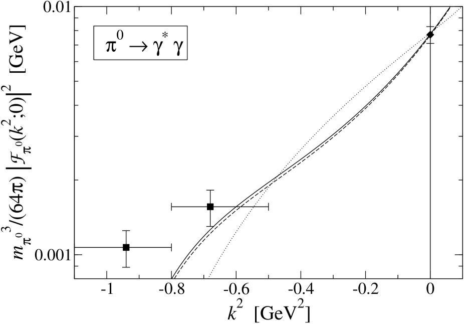
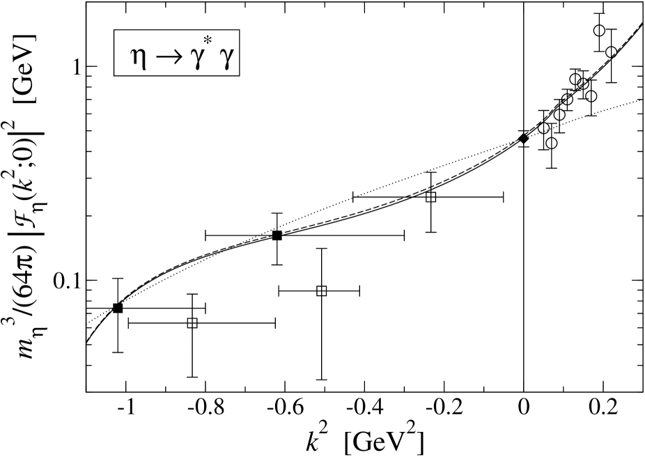
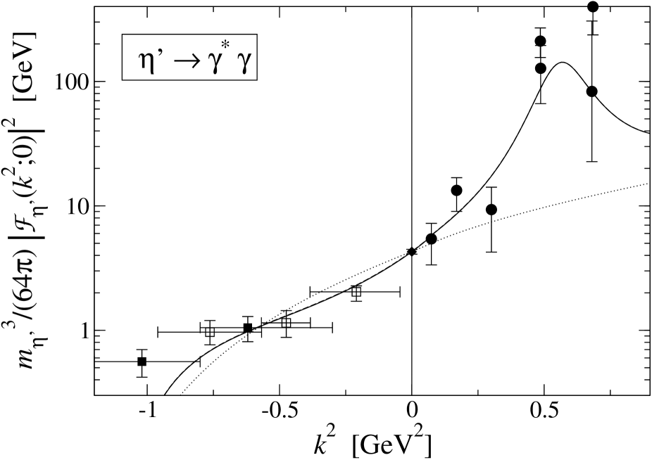
Figure 7: Results of the one-loop calculation (dotted), including the diagrams Figs. 6a+b (dashed), full calculation (solid). Data: solid squares [40], open squares [41], diamond [26], open circles [42], solid circles [43].

The overall good agreement with the data indicates that our model is capturing the important physics. In our fit, we have set the non-anomalous terms of unnatural parity at fourth chiral order to zero, $w_{1}^{(1)}=w_{2}^{(1)}=w_{3}^{(1)}=0$, since a good fit to the data can already be achieved without them, while keeping $F_{\eta^{\prime}}$ fixed at $F_{\eta^{\prime}}=1.1\;F_{\pi}$. Furthermore, we set the mixing parameter $\tilde{v}_{2}^{(1)}$ to zero which is consistent with a previous coupled channel calculation on hadronic decays of the $\eta$ and $\eta^{\prime}$ [19]. It should be emphasized that for a non-perturbative coupled channel approach the values of the coupling constants do not necessarily coincide with those from a perturbative loop-expansion, which was already pointed out in [19]. It is therefore not surprising that $\tilde{v}_{2}^{(1)}$ and the $w_{i}^{(1)}$ differ in both schemes. The inclusion of the diagrams in Figs. 6a, 6b which contain only one coupled channel and thus are associated with the exchange of only one vector-meson already yields the crucial structure of the curves (dashed line). The exchange of two vector-mesons (Fig. 6c) is merely a small correction which could even be compensated by a change of the parameters of the $\mathcal{O}(p^{6})$ counterterms. For completeness we have also shown the numerical results from the one-loop calculation which have been supplemented by the $k^{2}$ dependent counterterms at sixth chiral order, in order to be in better agreement for $k^{2}<0$. Due to this procedure the $k^{2}$ dependent terms differ from those in the coupled channel approach. Nevertheless, with this choice of parameters it is not possible to reproduce the sharp increase of the form factor for time-like photons, $k^{2}>0$, at the one-loop level, and we miss in any case the resonance structure in the $\eta^{\prime}$ decay.

The dependence of our results on the $\eta$-$\eta^{\prime}$ mixing parameter $\tilde{v}_{2}^{(1)}$ is depicted in Fig. 8. We have plotted the curves for different values of $\tilde{v}_{2}^{(1)}$, which indicate that a value for $\tilde{v}_{2}^{(1)}$ around zero is in better agreement with the data. The results for $\pi^{0}\to\gamma^{*}\gamma$ are, of course, not affected by changing $\tilde{v}_{2}^{(1)}$.

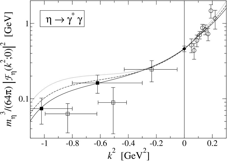
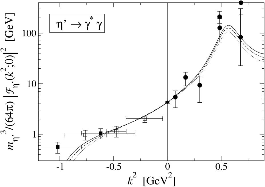
Figure 8: Dependence of $\mathcal{F}_{\eta}$ and $\mathcal{F}_{\eta^{\prime}}$ on the mixing parameter $\tilde{v}_{2}^{(1)}$: $\tilde{v}_{2}^{(1)}=0$ (solid), $\tilde{v}_{2}^{(1)}=0.5F_{\pi}^{2}/4$ (dashed), $\tilde{v}_{2}^{(1)}=1.15F_{\pi}^{2}/4$ (dotted).

In Fig. 9 we show our results for different values of the LEC $w_{3}^{(1)}$. When keeping $\tilde{v}_{2}^{(1)}=0$ only the process $\eta^{\prime}\to\gamma^{*}\gamma$ is altered. From the plot it can be seen that $w_{3}^{(1)}$ has significant influence on the peak structure at $k^{2}\approx 0.6\,\mathrm{GeV}^{2}$ and we can exclude values $w_{3}^{(1)}>2.0\times 10^{-3}$.

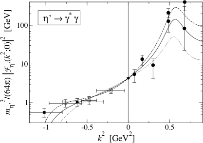
Figure 9: Dependence of $\mathcal{F}_{\eta^{\prime}}$ on the LEC $w_{3}^{(1)}$: $w_{3}^{(1)}=-3.0\times 10^{-3}$ (dashed), $w_{3}^{(1)}=0$ (solid), $w_{3}^{(1)}=3.0\times 10^{-3}$ (dotted).

Another quantity of interest is the slope parameter of the transition form factor. It is defined as the logarithmic derivative of the form factor $\mathcal{F}_{P}$ at $k^{2}=0$

$$b_{P}=\left.\frac{d}{dk^{2}}\ln{\mathcal{F}_{P}(k^{2};k^{\prime 2}=0)}\right|_{k^{2}=0}.$$ (61)

In Table 1 we compare our values with simple pole fits to the form factors. The value for $\pi^{0}$ is the world average given in [26]. For $\eta$ and $\eta^{\prime}$ we cite three measurements, the Lepton-G Collaboration [42, 43], the TPC/2$\gamma$ Collaboration [41] and the CELLO Collaboration [40]. From a pole fit a characteristic mass $\Lambda_{P}$ is extracted and related to the slope parameter via $b_{P}=1/\Lambda_{P}^{2}$. The obtained values are given by $\Lambda_{\eta}=(0.72\pm 0.09)\,\mathrm{GeV}$ [42], $\Lambda_{\eta}=(0.70\pm 0.08)\,\mathrm{GeV}$ [41], $\Lambda_{\eta}=(0.84\pm 0.06)\,\mathrm{GeV}$ [40] and $\Lambda_{\eta^{\prime}}=(0.77\pm 0.18)\,\mathrm{GeV}$ [43], $\Lambda_{\eta^{\prime}}=(0.85\pm 0.07)\,\mathrm{GeV}$ [41], $\Lambda_{\eta^{\prime}}=(0.79\pm 0.04)\,\mathrm{GeV}$ [40]. With one exception we achieve good agreement within error bars with the pole fits to the form factors. We point out that in the determination of the given errors for $b_{P}$ it has not been taken into account that in principle a different ansatz for the form factor can lead to different values of the slope parameter. In our model a significant part of the slope parameters is induced by the meson-meson rescattering processes. Again the exchange of two vector-mesons plays a negligible role.

	Experiment		NLO	1 CC	full
$\pi^{0}$	$1.76\pm 0.22$	[26]	1.19	1.98	1.95
	$1.9\pm 0.4$	[42]
$\eta$	$2.0\pm 0.5$	[41]	0.73	1.57	1.58
	$1.42\pm 0.21$	[40]
	$1.7\pm 0.8$	[43]
$\eta^{\prime}$	$1.38\pm 0.23$	[41]	0.85	1.78	1.79
	$1.59\pm 0.18$	[40]

Table 1: Slope parameters $b_{P}$ in units of $\,\mathrm{GeV}^{-2}$ derived from pole fits to the experimental data, the next-to-leading order calculation, including one coupled channel (diagrams Fig. 6a+b), and the full calculation.

Within our model, contributions from composed states of three pseudoscalar mesons which would correspond to the $\omega(782)$ have been neglected. However, the effects of the $\omega(782)$ should be similar to those of the $\rho(770)$ due to their almost equal masses. It may well be, that by keeping some of the analytic portions of the loop integrals in Eqs. (54,55) which amounts to a particular choice of higher order counterterms, we took into account the dynamical effects of the $\omega(782)$. Within our model, the contributions from the vector-mesons should thus be regarded to be a combination of both the $\omega(782)$ and the $\rho(770)$.

The contributions of the two vector-meson exchange diagrams, on the other hand, are almost negligible, as can be seen from Fig. 7. This is in sharp contradistinction to the complete Vector-Meson Dominance picture where the photons can only couple via the exchange of vector-mesons. Of course, when coupling to an on-shell photon the pertinent vector-meson propagator reduces to a vertex, but with both photons off-shell, the two approaches should yield different predictions. In Fig. 10 we show our predictions for two off-shell photons for $\pi^{0},\eta,\eta^{\prime}$ decays with $k^{2}=k^{\prime 2}$ as well as the $\eta^{\prime}$ transition form factor in the $(k^{2},k^{\prime 2})$-plane. As in the case with one off-shell photon the result of a calculation with one coupled channel is almost identical to the full calculation. A measurement of the transition form factors for two off-shell photons could serve as a check of our model and help to clarify, whether the exchange of only one or rather two vector-mesons occurs in these decays. For one and two off-shell photons with larger space-like momenta the pion transition form factor has been calculated within an instanton model of QCD [44]. For small negative photon virtualities the results are quite similar to ours.

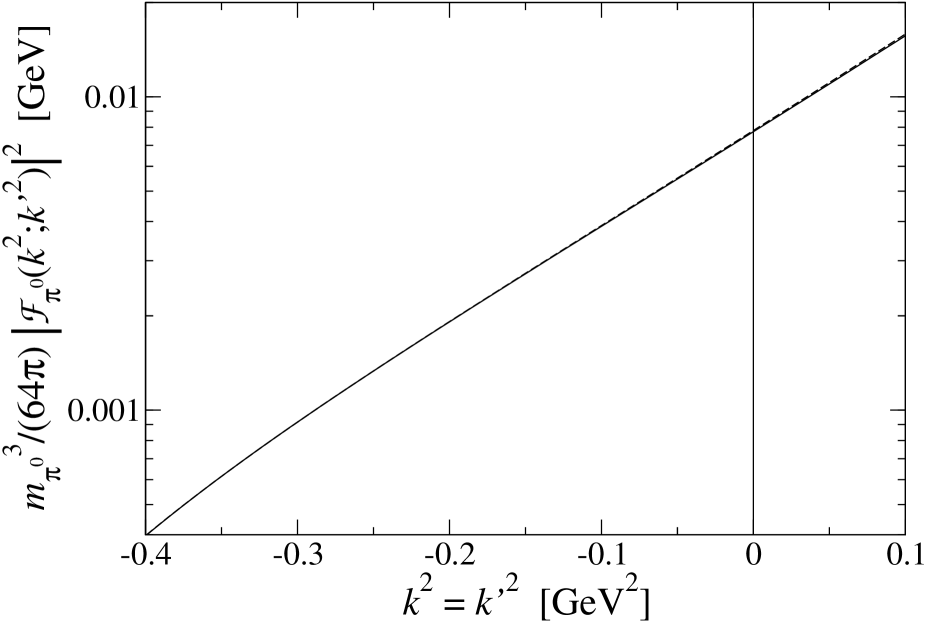
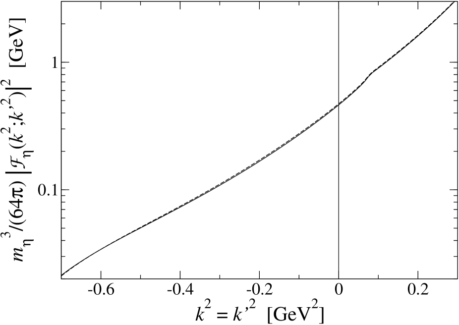
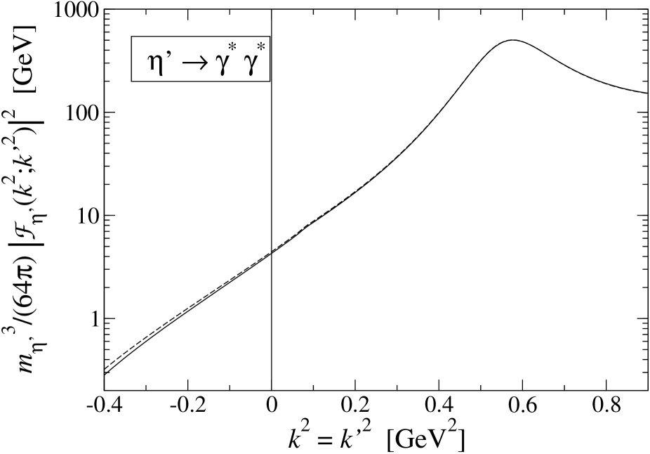
\begin{overpic}[width=386.95897pt]{3detap.eps} \put(15.0,7.0){\scalebox{0.8}{$k^{2}\ [\,\mathrm{GeV}^{2}]$}} \put(92.0,20.0){\scalebox{0.8}{$k^{\prime 2}\ [\,\mathrm{GeV}^{2}]$}} \put(-10.0,15.0){\rotatebox{90.0}{\scalebox{0.8}{$\ln{(m_{\eta^{\prime}}^{3}/(64\pi)|\mathcal{F}_{\eta^{\prime}}(k^{2};k^{\prime 2})|^{2})}$}}} \end{overpic}

Figure 10: Prediction of the transition form factors for two off-shell photons with $k^{2}=k^{\prime 2}$ resulting from the full calculation (solid) and from a calculation without the contribution from Fig. 6c with two coupled channels (dashed, almost on top of solid line). For $\eta^{\prime}\to\gamma^{*}\gamma^{*}$ we also show the transition form factor from the full calculation in the $(k^{2},k^{\prime 2})$-plane.

6 Conclusions

In the present work, we have investigated the two-photon decays of $\pi^{0},\eta$ and $\eta^{\prime}$ within a chiral unitary framework. To this end, we have supplemented the one-loop calculation of chiral perturbation theory by a Bethe-Salpeter approach which satisfies unitarity constraints and generates vector-mesons from composed states of two pseudoscalar mesons.

While the one-loop result is sufficient to achieve agreement with the decay widths $P\rightarrow\gamma\gamma$ $(P=\pi^{0},\eta,\eta^{\prime})$, the vector-meson exchange is crucial to reproduce the sharp increase of the transition form factor for time-like photons in the decays $P\rightarrow\gamma\gamma^{*}$. Our method reproduces also the resonance structure in the transition form factor of the decay $\eta^{\prime}\rightarrow\gamma\gamma^{*}$ at photon virtualities around $k^{2}\approx 0.6$ GeV².

Furthermore, our approach distinguishes between single and double vector-meson exchange, the latter one being the only contribution in the complete Vector-Meson Dominance picture. Our study suggests that for the decays with off-shell photons the exchange of one vector-meson is the dominant contribution, whereas the two vector-meson exchange is almost negligible which is in contradistinction to complete Vector-Meson Dominance. The available data on electromagnetic transition form factors is restricted to decays with exactly one off-shell photon. When coupling to an on-shell photon, the pertinent vector-meson propagator reduces to a vertex so that no clear distinction can be made between the two approaches. However, an experiment with two off-shell photons should be able to clarify, whether one or two vector-meson exchange occurs. The question whether double Vector-Meson Dominance holds is also an important issue for kaon decays and the anomalous magnetic moment of the muon. We have presented predictions for the decays with two off-shell photons, and again the exchange of two vector-mesons plays a minor role.

Within our model, contributions from composed states of three pseudoscalar mesons which would correspond to the $\omega(782)$ have been neglected. However, the effects of the $\omega(782)$ should be similar to those of the $\rho(770)$. It may well be, that by keeping some of the analytic portions of the loop integrals in our coupled channel analysis which amounts to a particular choice of higher order counterterms, we took into account the dynamical effects of the $\omega(782)$. Within our model, the contributions from the vector-mesons should thus be regarded to be a combination of both the $\omega(782)$ and the $\rho(770)$.

The present approach can be applied in a straightforward manner to the anomalous decays $\eta,\eta^{\prime}\rightarrow\pi^{+}\pi^{-}\gamma$ and the radiative decays $\eta,\eta^{\prime}\rightarrow\pi^{0}\gamma\gamma$ which will be investigated in future studies.

Appendix A Counterterms of order $\mathcal{O}(p^{6})$

In this section, we discuss the relevant counterterms of order $\mathcal{O}(p^{6})$. For the covariant derivative and the field strength tensors we use the following notation

$$\begin{array}[]{rcl}D_{\mu}U&=&\partial_{\mu}U-i\tilde{r}_{\mu}U+iU\tilde{l}_{\mu},\\[4.30554pt] \tilde{R}_{\mu\nu}&=&\partial_{\mu}\tilde{r}_{\nu}-\partial_{\nu}\tilde{r}_{\mu}-i[\tilde{r}_{\mu},\tilde{r}_{\nu}],\qquad\tilde{L}_{\mu\nu}=\partial_{\mu}\tilde{l}_{\nu}-\partial_{\nu}\tilde{l}_{\mu}-i[\tilde{l}_{\mu},\tilde{l}_{\nu}],\end{array}$$ (A.62)

where $\tilde{r}_{\mu}=v_{\mu}+\tilde{a}_{\mu}$, $\tilde{l}_{\mu}=v_{\mu}-\tilde{a}_{\mu}$ and $\tilde{a}_{\mu}=a_{\mu}+\frac{\sqrt{6\lambda}-f}{3f}\langle a_{\mu}\rangle$. The replacement of the original field strength tensors $R_{\mu\nu}$, $L_{\mu\nu}$ by the new quantities $\tilde{R}_{\mu\nu}$, $\tilde{L}_{\mu\nu}$ leads to additional counterterms which involve the derivative of the singlet component of the axial-vector field, $\langle\partial_{\mu}a_{\nu}\rangle$, however, such counterterms do not contribute to the processes discussed in the present work and are neglected.

In the $SU(3)$ framework there are numerous terms containing six derivatives which according to [24] can be reduced to only one contribution by utilizing methods such as partial integration, equation of motion, epsilon relations and Bianchi identities. In our notation it is given by

$$\begin{array}[]{ll}i\,\bar{W}_{1}\epsilon^{\mu\nu\alpha\beta}&\langle(2U^{\dagger}D^{\lambda}\tilde{R}_{\lambda\mu}U+2D^{\lambda}\tilde{L}_{\lambda\mu}+U^{\dagger}\tilde{R}_{\lambda\mu}D^{\lambda}U+D^{\lambda}U^{\dagger}\tilde{R}_{\lambda\mu}U+U^{\dagger}D^{\lambda}U\tilde{L}_{\lambda\mu}U^{\dagger}+\tilde{L}_{\lambda\mu}D^{\lambda}U^{\dagger}U)\\ &\quad\times\tilde{H}_{\nu\alpha}\,C_{\beta}\rangle,\end{array}$$ (A.63)

where we made use of the abbreviations

$$\begin{array}[]{rclrcl}\tilde{H}_{\mu\nu}&=&U^{\dagger}\tilde{R}_{\mu\nu}U+\tilde{L}_{\mu\nu},&C_{\mu}&=&U^{\dagger}D_{\mu}U,\\ M&=&U^{\dagger}\chi+\chi^{\dagger}U,&N&=&U^{\dagger}\chi-\chi^{\dagger}U.\end{array}$$ (A.64)

For the decays into two photons Eq. (A.63) yields the contribution (in the differential form notation of [5])

$$-\bar{w}_{1}^{(0)}\ \frac{16\sqrt{2}}{f}\ \langle\phi\ dv\ \square\,dv\rangle.$$ (A.65)

From the extension to the $U(3)$ framework there arise several more terms which reduce after applying the above mentioned methods to the relevant contribution

$$\bar{w}_{2}^{(1)}\,\frac{16}{f}\ \eta_{0}\ \langle dv\ \square\,dv\rangle.$$ (A.66)

Furthermore there are terms of order $\mathcal{O}(p^{6})$ that contain the chiral symmetry breaking object $\chi=2B\mathcal{M}$ with $\mathcal{M}$ being the quark mass matrix

$$\begin{array}[]{rccclccl}\mathcal{L}_{\chi}^{(6)}&=&&i\,\bar{W}_{3}&\epsilon^{\mu\nu\alpha\beta}\langle N\tilde{H}_{\mu\nu}\tilde{H}_{\alpha\beta}\rangle&+&i\,\bar{W}_{4}&\epsilon^{\mu\nu\alpha\beta}\langle N\rangle\langle\tilde{H}_{\mu\nu}\tilde{H}_{\alpha\beta}\rangle\\[4.30554pt] &&+&\bar{W}_{5}&\epsilon^{\mu\nu\alpha\beta}\langle M\tilde{H}_{\mu\nu}\tilde{H}_{\alpha\beta}\rangle&+&\bar{W}_{6}&\epsilon^{\mu\nu\alpha\beta}\langle M\rangle\langle\tilde{H}_{\mu\nu}\tilde{H}_{\alpha\beta}\rangle.\end{array}$$ (A.67)

The first two terms arise from conventional $SU(3)$ theory whereas the last two are due to the extension to $U(3)$. In the differential form notation the relevant contributions to the decay $P\to\gamma^{(*)}\gamma^{(*)}$ are given by the contact terms

$$\begin{array}[]{rcclcl}\mathcal{L}_{\chi,\,ct}^{(6)}&=&&\bar{w}_{3}^{(0)}\ \frac{32\sqrt{2}}{f}\langle\phi\,\chi\,dv\,dv\rangle&+&\bar{w}_{4}^{(0)}\ \frac{32\sqrt{2}}{f}\langle\phi\,\chi\rangle\langle dv\,dv\rangle\\[4.30554pt] &&+&\bar{w}_{5}^{(1)}\,\frac{32}{f}\ \eta_{0}\langle\chi\,dv\,dv\rangle&+&\bar{w}_{6}^{(1)}\,\frac{32}{f}\ \eta_{0}\langle\chi\rangle\langle dv\,dv\rangle.\end{array}$$ (A.68)

Combining all counterterms of order $\mathcal{O}(p^{6})$ we obtain

$$\mathcal{L}_{ct}^{(6)}=-\bar{w}_{1}^{(0)}\ \frac{16\sqrt{2}}{f}\ \langle\phi\ dv\ \square\,dv\rangle+\bar{w}_{2}^{(1)}\,\frac{16}{f}\ \eta_{0}\ \langle dv\ \square\,dv\rangle+\mathcal{L}_{\chi,\,ct}^{(6)}\ .$$ (A.69)

References

- [1] J. Wess and B. Zumino, Phys. Lett. B37 (1971) 95
- [2] E. Witten, Nucl. Phys. B223 (1983) 422
- [3] J. F. Donoghue, B. R. Holstein, and Y.-C. R. Lin, Phys. Rev. Lett. 55 (1985) 2766
- [4] J. Bijnens, A. Bramon, and F. Cornet, Phys. Rev. Lett. 61 (1988) 1453
- [5] R. Kaiser and H. Leutwyler, Eur. Phys. J. C17 (2000) 623
- [6] P. Herrera-Siklódy, Phys. Lett. B442 (1998) 359
- [7] J. F. Donoghue and D. Wyler, Nucl. Phys. B316 (1989) 289
- [8] J. Bijnens, A. Bramon, and F. Cornet, Z. Phys. C46 (1990) 599
- [9] J. Bijnens, Int. J. Mod. Phys. A8 (1993) 3045
- [10] H. Leutwyler, Nucl. Phys. Proc. Suppl. 64 (1998) 223
- [11] R. Kaiser and H. Leutwyler, “Pseudoscalar decay constants at large ”, in Proceedings of the Workshop Nonperturbative Methods in Quantum Field Theory, eds. A. W. Schreiber, A. G. Williams and A. W. Thomas (World Scientific, Singapore, 1998)
- [12] T. Feldmann and P. Kroll, Eur. Phys. J. C5 (1998) 327
- [13] T. Feldmann, P. Kroll and B. Stech, Phys. Rev. D 58 (1998) 114006
- [14] P. Herrera-Siklódy, J. I. Latorre, P. Pascual and J. Taron, Phys. Lett. B419 (1998) 326
- [15] N. Beisert and B. Borasoy, Eur. Phys. J. A11 (2001) 329
- [16] J. A. Oller and E. Oset, Nucl. Phys. A620 (1997) 438
- [17] J. A. Oller, E. Oset and J. R. Pelaez, Phys. Rev. D59 (1999) 074001
- [18] N. Beisert and B. Borasoy, Phys. Rev. D67 (2003) 074007
- [19] N. Beisert and B. Borasoy, Nucl. Phys. A716 (2003) 186
- [20] J. Bijnens, in Chiral Dynamics: Theory and Experiment, eds. A. M. Bernstein, D. Drechsel and T. Walcher, Mainz (1997), Springer
- [21] J. Gasser and H. Leutwyler, Nucl. Phys. B250 (1985) 465
- [22] B. Borasoy and S. Wetzel, Phys. Rev. D 63 (2001) 074019
- [23] J. L. Goity, A. M. Bernstein, B. R. Holstein, Phys. Rev. D66 (2002) 076014
-
[24]
D. Issler, Report SLAC-PUB-4943, 1990 (unpublished);
R. Akhoury and A. Alfakih, Ann. Phys. (N.Y.) 210 (1991) 81;
H. W. Fearing and S. Scherer, Phys. Rev. D53 (1996) 315;
J. Bijnens, L. Girlanda and P. Talavera, Eur. Phys. J. C23 (2002) 539;
T. Ebertshäuser, H. W. Fearing, S. Scherer, Phys. Rev. D65 (2002) 054033 - [25] J. Bijnens, G. Ecker and J. Gasser, in 2nd DANE Physics Handbook, eds. L. Maiani, G. Pancheri and N. Paver, INFN (1995), Frascati
- [26] Particle Data Group, K. Hagiwara et al., Phys. Rev. D66 (2002) 010001
- [27] B. Moussallam, Phys. Rev. D51 (1995) 4939
- [28] B. Ananthanarayan and B. Moussallam, JHEP 05 (2002) 052
- [29] M. Bando, T. Kugo, K. Yamawaki, Phys. Rept. 164 (1988) 217
- [30] T. Fujiwara et al., Prog. Theor. Phys. 73 (1985) 926
- [31] P. D. Ruiz-Femenía, A. Pich and J. Portolés, JHEP 07 (2003) 003
- [32] R. I. Dzhelyadin et al., Phys. Lett. B88 (1979) 379; B94 (1980) 548
- [33] H. Aihara et al., Phys. Rev. Lett. 64 (1990) 172
- [34] H. J. Behrend et al., Z. Phys C49 (1991) 401
- [35] J. A. Oller, U.-G. Meißner, Phys. Lett. B500 (2001) 263
- [36] T. Inoue, E. Oset, M. J. Vicente Vacas, Phys. Rev. C65 (2002) 035204
- [37] J. Nieves and E. Ruiz Arriola, Nucl. Phys. A679 (2000) 57
- [38] S. D. Protopopescu et al., Phys. Rev. D7 (1973) 1279
- [39] P. Estabrooks and A. D. Martin, Nucl. Phys. B79 (1974) 301
- [40] CELLO Coll. H.-J. Behrend et al., Z. Phys. C49 (1991) 401
- [41] TPC/2 Coll. H. Aihara et al., Phys. Rev. Lett. 64 (1990) 172
- [42] Lepton-G Coll. R. I. Dzhelyadin et al., Phys. Lett. B94 (1980) 548
- [43] Lepton-G Coll. R. I. Dzhelyadin et al., Phys. Lett. B88 (1979) 379
- [44] A. E. Dorokhov, JETP Lett. 77 (2003) 63