LAPTH-994

KEK-CP-142

Full ${\cal O}(\alpha)$ electroweak corrections to double Higgs-strahlung at the linear collider

G. Bélanger¹⁾, F. Boudjema¹⁾, J. Fujimoto²⁾, T. Ishikawa²⁾,

T. Kaneko²⁾, Y. Kurihara²⁾, K. Kato³⁾, Y. Shimizu²⁾

1) LAPTH${\;}^{\dagger}$, B.P.110, Annecy-le-Vieux F-74941, France.

2) KEK, Oho 1-1, Tsukuba, Ibaraki 305–0801, Japan.

3) Kogakuin University, Nishi-Shinjuku 1-24, Shinjuku, Tokyo 163–8677, Japan.

^†URA 14-36 du CNRS, associée à l’Université de Savoie.

1 Introduction

One of the primary goals of the first phase of a future $e^{+}e^{-}$ linear collider[1, 2, 3], LC, is a detailed precision study of the properties of the Higgs. According to the latest indirect precision data[4], one expects a rather light Higgs with a mass below the $W$ pair threshold. This is also within the range predicted for the lightest Higgs of the minimal supersymmetric model(MSSM). The LHC will be able to furnish a few measurements on the couplings of the Higgs to fermions and gauge bosons[5] but the most precise measurements will be performed in the clean environment of the linear collider. In order for these precision measurements to be feasible at the LC, the various observables need to be well under control theoretically. Nevertheless, although the branching ratios of the Higgs have been computed with great precision it is only during the last year that the one-loop electroweak radiative corrections to the main production channel at the LC, $e^{+}e^{-}\rightarrow\nu\bar{\nu}H$, has been achieved[6, 7, 8]. Even more recent is the calculation[9, 10, 11] of $e^{+}e^{-}\rightarrow t\bar{t}H$ which is crucial for the extraction of the important $t\bar{t}H$ vertex. Another important issue concerns the reconstruction of the Higgs potential which is the cornerstone of the electroweak symmetry breaking. Although measurements of the Higgs mass and its couplings to the fermions and bosons may give some information on this potential[12], a more direct probe is through the measurement of the Higgs self-couplings. In particular the tri-linear Higgs self-coupling, $HHH$, may be accessed in double Higgs production. Especially for the light Higgs mass this is a daunting task at the LHC[13, 14]. In $e^{+}e^{-}\;$the most promising channel in the first stage of a LC, double Higgs-strahlung, $e^{+}e^{-}\rightarrow ZHH\;$[15, 16], seems to be the most promising. The aim of this letter is to give the full electroweak correction to this process, thus adding to the precision calculations of the Higgs profile at the LC.

The cross sections for $e^{+}e^{-}\rightarrow ZHH\;$are rather small reaching about $0.2$fb at centre of mass energies around $500$GeV and for Higgs masses in the interesting range $110<M_{H}<130$GeV as suggested by supersymmetry. However detailed simulations[17] including the issue of backgrounds have shown that a precision of about $10\%$ on the total cross section can be achieved with a collected luminosity of $1$ab^-1 especially if a neural networks analysis is performed. Other simulations[18, 19] have shown that by using some discriminating kinematics variables, namely the invariant mass of the $HH$ system, one can further improve the extraction of the Higgs self-coupling $\lambda_{HHH}$. It is important to point out that although the foreseen experimental precision on the cross section is about $10\%$, the knowledge of the complete ${\cal O}(\alpha)\;$corrections is mandatory for this process. Indeed we already know that the radiative corrections to the Higgs self-couplings alone, which is just a small subset of the full electroweak corrections, receive a $M_{t}^{4}$ correction and are therefore potentially large, with $M_{t}$ being the top mass. The leading correction to the tree-level $\lambda_{HHH}^{(0)}$ coupling writes

$$\lambda_{HHH}=\lambda_{HHH}^{0}\left(1-\frac{\alpha}{\pi s_{W}^{2}}\frac{M_{t}^{4}}{M_{W}^{2}M_{H}^{2}}\right),\quad s_{W}^{2}=1-M_{W}^{2}/M_{Z}^{2}.$$ (1)

$M_{W}$ and $M_{Z}$ are, respectively, the $W$ mass and $Z$ mass and $\alpha$ the fine structure constant. For $M_{H}=120$GeV, this constitutes as much as $-10\%$ correction to the tri-linear Higgs coupling. Although the contribution from diagrams from the triple Higgs vertex to the full process are not the dominant ones, this correction alone can amount to about $-5\%$ to the total cross section[15].

2 Grace-Loop and the calculation of $e^{+}e^{-}\rightarrow ZHH\;$

2.1 Checks on the one-loop result

Our computation is performed with the help of GRACE-loop[21]. This is a code for the automatic generation and calculation of the full one-loop electroweak radiative corrections in the ${\cal{S}}{\cal{M}}$. The code has successfully reproduced the results of a host of one-loop $2\rightarrow 2$ electroweak processes[21]. GRACE-loop also provided the first results on the full one-loop radiative corrections to $e^{+}e^{-}\rightarrow\nu\bar{\nu}H$ [6, 7] and more recently on $e^{+}e^{-}\rightarrow t\bar{t}H\;$[9]. Both these calculations have now been confirmed by an independent calculation[8, 10]. For all electroweak processes we adopt the on-shell renormalisation scheme according to[7, 21, 22]. For each process some stringent consistency checks are performed. The results are checked by performing three kinds of tests at some random points in phase space. For these tests to be passed one works in quadruple precision. Details of how these tests are performed are given in[7, 21]. Here we only describe the main features of these tests.
i) We first check the ultraviolet finiteness of the results. This test applies to the whole set of the virtual one-loop diagrams. In order to conduct this test we regularise any infrared divergence by giving the photon a fictitious mass (for this calculation we set this at $\lambda=10^{-21}$GeV). In the intermediate step of the symbolic calculation dealing with loop integrals (in $n$-dimension), we extract the regulator constant $C_{UV}=1/\varepsilon-\gamma_{E}+\log 4\pi$, $n=4-2\varepsilon$ and treat this as a parameter. The ultraviolet finiteness test is performed by varying the dimensional regularisation parameter $C_{UV}$. This parameter could then be set to $0$ in further computation. Quantitatively for the process at hand, the ultraviolet finiteness test gives a result that is stable over $29$ digits when one varies the dimensional regularisation parameter $C_{UV}$.

ii) The test on the infrared finiteness is performed by including both the loop and the soft bremsstrahlung contributions and checking that there is no dependence on the fictitious photon mass $\lambda$. The soft bremsstrahlung part consists of a soft photon contribution where the external photon is required to have an energy $k_{\gamma}^{0}<k_{c}\ll E_{b}$. $E_{b}$ is the beam energy. This part factorises and can be dealt with analytically. For the QED infrared finiteness test we also find results that are stable over $23$ digits when varying the fictitious photon mass $\lambda$.

iii) A crucial test concerns the gauge parameter independence of the results. Gauge parameter independence of the result is performed through a set of five gauge fixing parameters. For the latter a generalised non-linear gauge fixing condition[21] has been chosen,

$${{\cal L}}_{GF} = -\frac{1}{\xi_{W}}|(\partial_{\mu}\;-\;ie\tilde{\alpha}A_{\mu}\;-\;igc_{W}\tilde{\beta}Z_{\mu})W^{\mu+}+\xi_{W}\frac{g}{2}(v+\tilde{\delta}H+i\tilde{\kappa}\chi_{3})\chi^{+}|^{2}$$ (2)

$$\;-\frac{1}{2\xi_{Z}}(\partial.Z+\xi_{Z}\frac{g}{2c_{W}}(v+\tilde{\varepsilon}H)\chi_{3})^{2}\;-\frac{1}{2\xi_{A}}(\partial.A)^{2}\;.$$

The $\chi$ represents the Goldstone. We take the ’t Hooft-Feynman gauge with $\xi_{W}=\xi_{Z}=\xi_{A}=1$ so that no “longitudinal” term in the gauge propagators contributes. Not only this makes the expressions much simpler and avoids unnecessary large cancellations, but it also avoids the need for high tensor structures in the loop integrals. The use of the five parameters, $\tilde{\alpha},\tilde{\beta},\tilde{\delta},\tilde{\kappa},\tilde{\varepsilon}$ is not redundant as often these parameters check complementary sets of diagrams. Let us also point out that when performing this check we keep the full set of diagrams including couplings of the Goldstone and Higgs to the electron for example, as will be done for the process under consideration. Only at the stage of integrating over the phase space do we switch these negligible contributions off. Here, the gauge parameter independence checks give results that are stable over $27$ digits (or better) when varying any of the non-linear gauge fixing parameters.

2.2 The five point function

The gauge invariance check is also a very powerful check as concerns the reduction of the various tensor integrals down to the scalar integrals of rank $N$. For $N<5$ we perform this reduction in terms of Feynman parameters as detailed in our review[21]. As for the scalar $N=3,4$ integrals we use the FF package[23]. The implementation of the scalar five-point function is done exactly as in our previous paper on $e^{+}e^{-}\rightarrow\nu\bar{\nu}H\;$[7]. On the other hand we have improved the algorithm for the reduction of the tensor integrals for the five point function. A general five point function is constructed out of tensor five point functions and is written as

$$T^{(5)}=\int\frac{d^{n}l}{(2\pi)^{n}}\;\frac{N(l)}{D_{0}D_{1}\cdots D_{4}}=G^{\mu\nu\cdots\rho}\;\int\frac{d^{n}l}{(2\pi)^{n}}\;\frac{\overbrace{l_{\mu}l_{\nu}\cdots l_{\rho}}^{M}}{D_{0}D_{1}\cdots D_{4}},\quad M\leq 5,$$ (3)

where

$$D_{0}=l^{2}-M_{0}^{2}\quad D_{i}=(l+s_{i})^{2}-M_{i}^{2},\quad s_{i}=\sum_{j=1}^{i}p_{j},\qquad i=1,2,3,4.$$ (4)

$M_{i}$ are the internal masses, $p_{i}$ the set (of linearly independent) incoming momenta, $l$ the loop momentum and $G^{\mu\nu\cdots\rho}$ a tensor that involves the external momenta, the metric or anti-symmetric tensors. The scalar integral has $N(l)=1$.
Because the set $s_{i}$ forms a basis for vectors in 4-dimensional space, introducing the Gram matrix $A_{ij}=s_{i}.s_{j}$ one has the identities

$$g^{\mu\nu}=\sum_{i,j=1}^{4}s_{i}^{\mu}A_{ij}^{-1}s_{j}^{\nu},\quad l^{\mu} = \sum_{i,j}s_{i}^{\mu}A^{-1}_{ij}(l.s_{j}).$$ (5)

We then rewrite an occurrence of $l^{2}$ in $N(l)$ in terms of $D_{0}$. For a term with $l_{\mu}$ we use Eq.(5) and re-express $l.s_{j}$ as a difference of $D_{j}$ and $D_{0}$ (and loop momenta independent terms). Using this trick one is able to write

$$N(l) = \sum_{\alpha=0}^{4}E_{\alpha}(l)D_{\alpha}+F,$$

where $F$ is independent of the loop momentum and corresponds then to the scalar five-point function which we treat as in[7]. The terms proportional to $D_{\alpha}$ correspond to a tensor four-point function of rank-$M-1$ or $M-2$, starting from a rank-$M$ in the original $T^{(5)}$. We use REDUCE for extracting $E(l)$ and $F$ analytically. This new algorithm can provide much shorter matrix elements compared with the previous one, which used the identity

$$l^{2} = \sum_{i,j}(l.s_{i})A^{-1}_{i,j}(l.s_{j}),$$

instead of $l_{\mu}$ in Eq.(5).

2.3 Input parameters

Our input parameters for the calculation of $e^{+}e^{-}\rightarrow ZHH$ are the following. We will start by presenting the results of the electroweak corrections in terms of the fine structure constant in the Thomson limit with $\alpha^{-1}=137.0359895$ and the $Z$ mass $M_{Z}=91.1876$ GeV. The on-shell renormalisation program, which we have described in detail elsewhere[21], uses $M_{W}$ as an input. However, the numerical value of $M_{W}$ is derived through $\Delta r$[24] with $G_{\mu}=1.16639\times 10^{-5}{\rm GeV}^{-2}$. Thus, $M_{W}$ changes as a function of $M_{H}$. For the lepton masses we take $m_{e}=0.510999$ MeV, $m_{\mu}=105.658389$ MeV and $m_{\tau}=1.7771$ GeV. For the quark masses, beside the top mass $M_{t}=174$ GeV, we take the set $M_{u}=M_{d}=63$ MeV, $M_{s}=94$ MeV, $M_{c}=1.5$ GeV and $M_{b}=4.7$ GeV. With this we find, for example, that $M_{W}=80.3766$GeV ($\Delta r=2.549\%$) for $M_{H}=120$ GeV and $M_{W}=80.3477$GeV ($\Delta r=2.697\%$) for $M_{H}=180$ GeV.

As well known, from the direct experimental search of the Higgs boson at LEP2, the lower bound of the ${\cal{S}}{\cal{M}}\;$Higgs boson mass is 114.4 GeV[26]. On the other hand, indirect study of the electroweak precision measurement suggests that the upper bound of the ${\cal{S}}{\cal{M}}\;$Higgs mass is about 200 GeV[4]. In this paper, we therefore only consider a relatively light ${\cal{S}}{\cal{M}}\;$Higgs boson and take the illustrative values $M_{H}=120$GeV, $M_{H}=150$GeV and $M_{H}=180$GeV. In fact already for $M_{H}>2M_{W}$ the process loses its interest for the LC as not only the cross section decreases but also because the dominant decay mode of the Higgs into $W$’s precludes a precision study[14] of the triple Higgs coupling.

2.4 Overview of the Feynman diagrams

The full set of the Feynman diagrams within the non-linear gauge fixing condition consists of 27 tree-level diagrams and as many as 5417 one-loop diagrams for the electroweak ${\cal O}(\alpha)$ correction to $e^{+}e^{-}\rightarrow ZHH$, see Fig. 1 for a selection of these diagrams. Neglecting the electron-Higgs coupling, the set of diagrams still includes 6 tree-level diagrams and 1597 one-loop diagrams. We define this latter set as the production set. To obtain the results of the total cross sections, we use this production set.

Figure 1: A small selection of different classes of loop diagrams contributing to $e^{+}e^{-}\rightarrow ZHH\;$. We keep the same graph numbering as that produced by the system. The first three graphs represent corrections to the $HHH$ vertex. Graph 720 and Graph 805 are box corrections representing $Z^{\star},\gamma^{\star}\rightarrow HHZ$. Graph 3369 is a $t$-channel induced diagram with $W^{+}W^{-}\rightarrow ZH^{\star}$ as a subprocess. Graph 3417 is a typical pentagon diagram. Graph 5415 is a two-point function correction. We do not show the QED graphs as they amount to dressing the vertex $e^{+}e^{-}Z^{\star}$.

3 Results

3.1 Tree-level

To set the stage and to help understand the behaviour of the QED corrections, let us first give a brief summary on the cross section at tree-level. This is shown in Fig. 2.

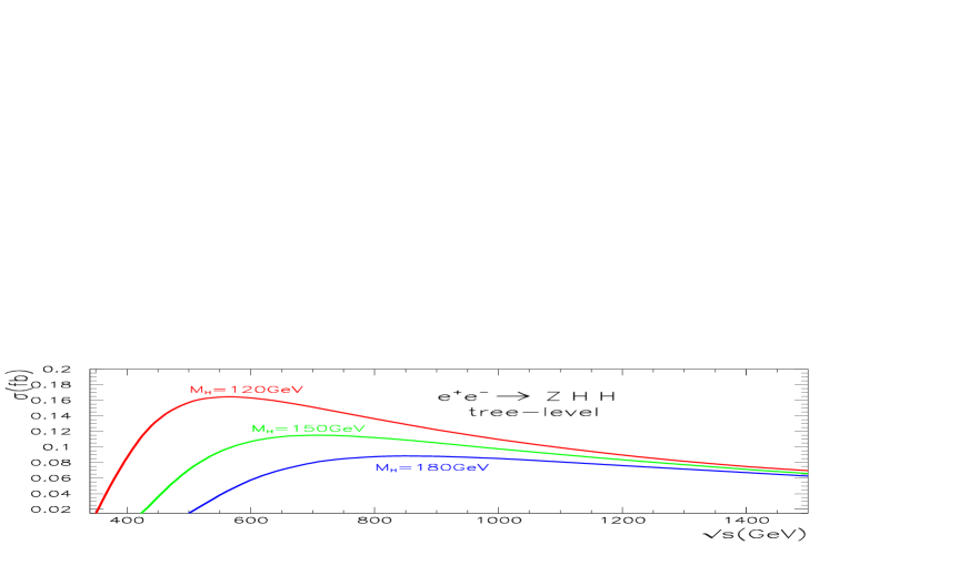
Figure 2: Total cross section for $e^{+}e^{-}\rightarrow ZHH\;$as a function of the centre of mass energy for $M_{H}=120,150,180$GeV.

Especially for the lightest Higgs mass, $M_{H}=120$GeV, there is a sharp increase right after threshold. For this particular Higgs mass the peak cross section is about $0.16$fb, at higher energies the cross section decreases rather sharply. This peak cross section decreases with increasing Higgs masses. Note, for further reference, that for energies below $\sim 1.2$TeV there is a rather strong dependence on the Higgs mass even in the restricted range of Higgs masses that we are studying. For the measurement of the $HHH$ coupling it is most useful to run at the maximum of the cross section. For a total integrated luminosity of $1$ab^-1 the $1\sigma$ statistical error corresponds to about a $2\%$ precision. Thus the theoretical knowledge of the cross section at $0.2\%$ is more than sufficient. Expectedly at high energies, the cross section shows little dependence on the Higgs mass, at $\sqrt{s}=1.5$TeV, the cross section is about $0.06$fb.

3.2 QED corrections: Slicing vs subtracting

In our description of the computation of the one-loop virtual electroweak corrections, the soft QED bremsstrahlung contribution introduces the soft-photon cut-off parameter $k_{c}$. The $k_{c}$ dependence drops out when calculating the full ${\cal O}(\alpha)\;$by including the hard photon part, $d\sigma_{H}\equiv d\sigma_{e^{+}e^{-}\rightarrow ZHH\gamma}(k_{\gamma}^{0}>k_{c})$. With $\delta_{V}=\delta_{V}^{EW}+\delta_{V}^{QED}$ the virtual loop correction (including weak and QED corrections), the total (integrated) ${\cal O}(\alpha)\;$correction writes

$$\sigma_{{\cal O}(\alpha)} = \sigma_{0}(1+\delta_{{\cal O}(\alpha)})=\int d\sigma_{0}\left(1+\delta_{V}+\delta_{S}(k_{c})\right)+\int d\sigma_{H}(k_{c}),$$ (6)

$$= \underbrace{\int d\sigma_{0}\left(1+\delta_{V}^{EW}\right)}_{\sigma_{0}(1+\delta_{W})}+\underbrace{\int d\sigma_{0}\left(\delta_{V}^{QED}+\delta_{S}(k_{c})\right)}_{\sigma_{V+S}^{QED}(k_{c})}+\underbrace{\int d\sigma_{H}(k_{c})}_{\sigma_{H}(k_{c})}$$

$$= \sigma_{0}(1+\delta_{W}+\delta_{{\rm QED}}).$$

The second and third terms define our default slicing method. The factorised soft-photon correction $d\sigma_{S}$ writes as

$$d\sigma_{S} = d\sigma_{0}\cdot\delta_{S}(k_{c})=d\sigma_{0}\cdot f_{LL}(k_{\gamma}^{0}<k_{c})$$ (7)

with $d\sigma_{0}$ the tree-level $2\rightarrow 3$ differential cross section and the radiator function $f_{LL}$ is defined through

$$f_{LL} = -e^{2}\;\int\frac{d^{3}k_{\gamma}}{(2\pi)^{3}2k_{\gamma}^{0}}\left|\frac{p^{-}}{k_{\gamma}\cdot p^{-}}-\frac{p^{+}}{k_{\gamma}\cdot p^{+}}\right|^{2},$$ (8)

where $k_{\gamma}(p^{\pm})$ are photon ($e^{\pm}$) 4-momenta. As a default in GRACE-loop the hard photon contribution is performed by the adaptive Monte-Carlo integration BASES[27] and the exact matrix elements are generated by GRACE. We then check that within the Monte-Carlo integration errors there is no $k_{c}$ dependence, usually at the per-mil level or even better (see below). For practically all $2\rightarrow 3$ processes this is sufficient.

For the process at hand we have also introduced a second method for the calculation of the hard part. A difficulty stems from the large contribution from the collinear regions, ${\cal O}(m_{e}^{2}/s)$, (of the hard photon radiation) which cancels a large part of the negative contribution from $\delta_{V+S}^{QED}=\delta_{V}^{QED}+\delta_{S}$. In order to have a more stable result we use a subtraction technique[28] which is a variant of the dipole subtraction introduced in [29] for QCD and in [30] for photon radiation. The idea is to add and subtract to $d\sigma_{H}(k_{c})$ a function that captures the leading contribution of $d\sigma_{H}(k_{c})$ and which is much easier to integrate. In our case we use the function $d\tilde{\sigma}_{0}\otimes f_{LL}$, where $d\tilde{\sigma}_{0}$ is derived from the tree-level $d\sigma_{0}$ but with kinematics taking into account the radiative photon emission. $\otimes$ stands for the phase-space integration of the radiative photon convoluted with 3-body phase-space of the tree-level cross-section. Therefore we explicitly write

$$\sigma_{{\cal O}(\alpha)} = \int d\sigma_{0}\left(1+\delta_{V}+\delta_{S}\right)+\int d\tilde{\sigma}_{0}\otimes f_{LL}(k_{\gamma}^{0}>k_{c})$$

$$+ \int\left(d\sigma_{H}(k_{\gamma}^{0}>k_{c})-d\tilde{\sigma}_{0}\otimes f_{LL}(k_{\gamma}^{0}>k_{c})\right)$$

$$\equiv \sigma_{0}\left(1+\delta_{W}\right)+\underbrace{\int\left(d\sigma_{0}\;\delta_{V}^{{\rm QED}}+d\tilde{\sigma}_{0}\otimes f_{LL}\right)}_{\sigma^{QED}_{A}}+\underbrace{\int\left(d\sigma_{H}(k_{\gamma}^{0}>k_{c})-d\tilde{\sigma}_{0}\otimes f_{LL}(k_{\gamma}^{0}>k_{c})\right)}_{\sigma^{QED}_{B}}$$

In $\sigma^{QED}_{A}$ of Eq.(3.2), the convolution over the photon now includes both hard and soft photon emission. The two-dimensional integration over the radiator $f_{LL}$ is performed with the help of the Good Lattice Point quasi Monte-Carlo method, see for example [31] for a description of this method. This ensures appropriate cancellations of the singularities between the loop and bremsstrahlung corrections at each point of (the tree-level) phase-space. All integration over the remaining tree-level differential cross section including both the virtual loop corrections and photon emission is done with BASES. For $\sigma^{QED}_{B}$ we also use BASES adapted to a $2\rightarrow 4$ process. Here the subtraction means that all singularities are made smooth at each point in phase space.

For the process at hand, which at tree-level proceeds through $s$-channel $Z$-exchange, the virtual QED corrections form a gauge invariant set which is all contained in the $e^{+}e^{-}Z^{\star}$ vertex. The dominant initial state QED virtual and soft bremsstrahlung corrections are given by the universal soft photon factor that leads to a relative correction[7]

$$\delta_{V+S}^{QED}=\frac{2\alpha}{\pi}\left((L_{e}-1)\ln\frac{k_{c}}{E_{b}}+\frac{3}{4}L_{e}+\frac{\pi^{2}}{6}-1\right),\quad\;L_{e}=\ln(s/m_{e}^{2})\;,$$ (10)

where $m_{e}$ is the electron mass, $E_{b}$ the beam energy ($s=4E_{b}^{2}$) and $k_{c}$ is the cut on the soft photon energy.

Although this approach of extracting the full QED correction is the most simple one, we have also calculated the full QED corrections separately and subtracted their contributions from the full ${\cal O}(\alpha)$. In order to perform this subtraction, the QED virtual corrections are generated by dressing the tree-level diagrams with one-loop photons (the photon self-energy is not included in this class). Moreover one needs to include some counterterms. One only has to take into account the purely photonic contribution to the wave function renormalisation constants of the electron. Performing this more direct computation is another test on the system.

$\sqrt{s}$	$\sigma_{\rm tree}=\int d\sigma_{0}$	$\sigma^{QED}_{A}$	$\sigma^{QED}_{B}$	$\delta_{QED}^{\prime}$	$\int d\sigma_{V+S}^{QED}(k_{c})$	$\int d\sigma_{H}(k_{c})$	$\delta_{QED}$
[GeV]	[fb]	[fb]	[fb]	[%]	[fb]	[fb]	[%]
$400$	$0.08644$	$-0.01636$	$0.00007$	$-18.84$	$-0.11971$	$0.10344$	$-18.83$
$600$	$0.16312$	$-0.00743$	$0.00155$	$-3.61$	$-0.24122$	$0.23535$	$-3.60$
$800$	$0.13631$	$-0.00075$	$0.00284$	$1.53$	$-0.21091$	$0.21300$	$1.53$
$1000$	$0.10985$	$0.00130$	$0.00344$	$4.32$	$-0.17594$	$0.18067$	$4.31$
$1500$	$0.06983$	$0.00201$	$0.00360$	$8.02$	$-0.11887$	$0.12448$	$8.04$

Table 1: Comparison between the results of the subtraction method and the slicing method as described in the text for totally integrated quantities. $M_{H}=120$GeV and $k_{c}=10^{-3}$GeV. $\delta_{QED}^{\prime}$($\delta_{QED}$) is the percentage total QED correction in the subtraction (slicing) method.

Table 1 shows a comparison of the total QED correction in our default slicing method and our numerical implementation of the subtraction method. We see that the agreement is excellent (at the level of $10^{-4}$ accuracy). The table also makes clear the advantage of the subtraction method in that no large cancellation between the part containing the virtual contribution and the rest occurs, moreover both are much smaller than the two parts obtained in the slicing method. There, as advertised, a large cancellation takes part. We note also that $\int d\sigma_{V+S}^{QED}(k_{c})$ in Table 1, is in excellent agreement with the result obtained by multiplying the tree-level cross section with the universal factor of Eq.(10). It is important to note that the full QED correction are rather large and negative around threshold, moderate around the peak and increase steadily for high energies. Most of this can be explained from the behaviour of the tree-level cross section, see Fig. 2, as a boost (sort of a radiative return) towards lower energies.

3.3 The genuine weak corrections

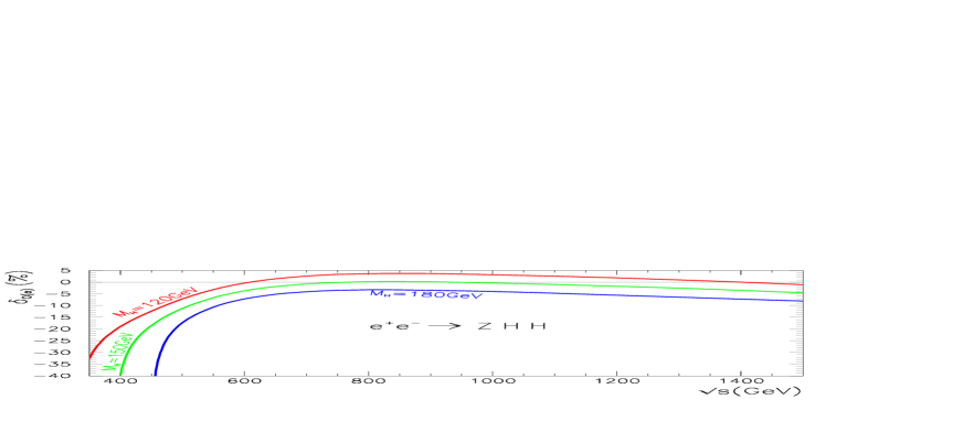
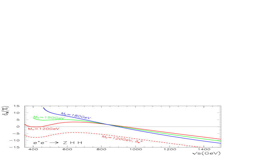
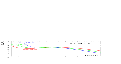
Figure 3: The full ${\cal O}(\alpha)$ relative correction (top panel) and the relative electroweak correction $\delta_{W}$ (lower panel) as a function of energy for $M_{H}=120,150,180$GeV. In addition, the genuine weak correction $\delta_{W}^{G}$ in the $G_{\mu}$ scheme is presented for $M_{H}=120$GeV (dotted line). The insert shows $\delta_{W}$ for $e^{+}e^{-}\rightarrow ZH$ for the same three Higgs masses.

We now turn to the genuine weak corrections which are the most interesting from a physics point of view. We have already discussed how in this process these corrections can be unambiguously defined. The total ${\cal O}(\alpha)\;$correction and the genuine weak corrections as a function of energy for our three representative Higgs masses are shown in Fig. 3.

$\sqrt{s}$	$M_{H}$(GeV)	$\sigma_{tree}$(fb)	$\Delta\sigma_{{\cal O}(\alpha)}$(fb)	$\delta_{{\cal O}(\alpha)}(\%)$	$\delta_{W}(\%)$
600 GeV	120	$1.6311(2)\times 10^{-1}$	$-0.719(3)\times 10^{-3}$	$-0.44(1)$	$3.17(1)$
	150	$1.0704(1)\times 10^{-1}$	$-3.987(3)\times 10^{-3}$	$-3.72(1)$	$5.14(1)$
	180	$5.7491(5)\times 10^{-2}$	$-4.136(3)\times 10^{-3}$	$-7.19(1)$	$7.60(1)$
800 GeV	120	$1.3631(1)\times 10^{-1}$	$+4.911(6)\times 10^{-3}$	$3.60(1)$	$2.07(1)$
	150	$1.1221(1)\times 10^{-1}$	$-0.167(8)\times 10^{-3}$	$0.14(1)$	$2.27(1)$
	180	$8.7604(8)\times 10^{-2}$	$-2.917(6)\times 10^{-3}$	$-3.33(1)$	$2.45(1)$
1 TeV	120	$1.0986(1)\times 10^{-1}$	$+3.462(6)\times 10^{-3}$	$3.15(1)$	$-1.17(1)$
	150	$9.7667(9)\times 10^{-2}$	$-0.386(8)\times 10^{-4}$	$-0.40(1)$	$-1.78(1)$
	180	$8.5245(8)\times 10^{-2}$	$-3.413(9)\times 10^{-3}$	$-4.00(1)$	$-2.54(1)$

Table 2: Total ${\cal O}(\alpha)$ and genuine weak corrections.

Specialising first to $M_{H}=120$GeV, the genuine weak corrections expressed in the $\alpha$-scheme are very small at threshold and also for energies corresponding to the peak cross section. At threshold this is in sharp contrast to the full ${\cal O}(\alpha)\;$cross section which is overwhelmingly dominated by the pure QED correction. For the range of the most interesting centre of mass energies where the cross section is largest, the (relative) weak correction is never more than $4\%$. Notice also the “spoon-like” behaviour of the weak correction at the lowest energies. This also occurs in $e^{+}e^{-}\rightarrow ZH$ as displayed in the insert of Figure 3 and has also been observed in the so-called $s$-channel of $e^{+}e^{-}\rightarrow\nu\bar{\nu}H$ (see Fig. 3a of[7]). This seems to be due to a competition between the bosonic and fermionic contributions at energies close to threshold but a more detailed investigation is needed to confirm the origin of this common feature. Passed the peak, the weak correction steadily turns negative reaching about $-10\%$ at $1.5$TeV. Comparing to the case with $M_{H}=150$GeV and $M_{H}=180$GeV, we see that, in fact, past $\sqrt{s}=800$GeV, the Higgs mass dependence of the genuine electroweak correction is small. Larger differences between the 3 Higgs masses considered here only appear for the smallest energies around threshold. Like for $M_{H}=120$GeV, for both $M_{H}=150$ and $M_{H}=180$GeV the weak correction around the peak is also within about $5\%$ and thus well contained. Note that the decrease of the weak correction as the energy increases is faster with the higher Higgs mass, a trend which is similar to that inherited from $e^{+}e^{-}\rightarrow ZH$ (see insert of Figure 3).
Having subtracted the genuine weak corrections one could also express the corrections in the $G_{\mu}$ scheme by further extracting the rather large universal weak corrections that affect two-point functions through $\Delta r$. This defines the genuine weak corrections in the $G_{\mu}$ scheme as $\delta_{W}^{G}=\delta_{W}-3\Delta r$. For $e^{+}e^{-}\rightarrow\nu\bar{\nu}H\;$this procedure helps absorb a large part of the weak corrections. Another advantage is that much of the (large) dependence due to the light fermions masses also drops out. However one sees, Fig. 3, that especially for high energies, this scheme fails to properly encapsulates the bulk of the radiative corrections. This is akin to what happens in $e^{+}e^{-}\rightarrow ZH\;$[32] and $e^{+}e^{-}\rightarrow t\bar{t}H$[9] where the bosonic weak corrections become important (and negative) at high energies.
To summarise it is perhaps worth to stress that if the total cross section even at its peak value would not be measured better than $10\%$ it would then be difficult to observe the genuine weak corrections. One should also observe that the approximate leading top mass correction to the Higgs self-couplings as given in Eq. (1) and which has no energy dependence can not reproduce the bulk of the weak correction.

3.4 Corrections to the $M_{HH}$ distribution

Figure 4: $d\sigma/dM_{HH}$ for $M_{H}=120$GeV at $\sqrt{s}=1$TeV. We show the tree-level (full curve), the effect of including only the genuine weak corrections (dotted curve) and the effect of including the full ${\cal O}(\alpha)\;$(dashed curve).

The $M_{HH}$ distribution has been shown[18, 19] to be a good discriminator for isolating the $HHH$ vertex, taking advantage of the fact that the two final Higgs mimic the decay product of a scalar (the virtual Higgs in the $HHH$ vertex)[16]. It is therefore important to enquire how this distribution gets affected by loop corrections. We have chosen as an illustrative case, $M_{H}=120$GeV at a centre of mass energy $\sqrt{s}=1$TeV which is the same configuration that was studied recently in the simulation of [19] which included, at tree-level, the effect of an anomalous triple Higgs coupling. In there it was shown that a deviation in this coupling affects primarily the lower end of the $M_{HH}$ spectrum, whereas the higher end is little affected. This is rather similar to the effect of the full ${\cal O}(\alpha)\;$correction as shown in Fig. 4 especially at the lower edge of the spectrum. The full ${\cal O}(\alpha)\;$correction, which for the integrated cross section reaches about $+3\%$, shows in fact a depletion from the higher $M_{HH}$ to the lower $M_{HH}$ values, again an effect due to the radiative return. After extracting the QED correction, the distribution including the weak corrections is hardly, considering the foreseen precision, noticeable though. Therefore we conclude that an anomalous coupling could still be distinguished, if large enough, in this distribution provided a proper inclusion of the initial QED corrections is allowed for in the experimental simulation.

4 Conclusions

We have performed a full one-loop correction to the process $e^{+}e^{-}\rightarrow ZHH$. This is a process which is interesting and of importance mainly because it gives access to the measurement of the triple Higgs coupling. Our calculation shows that especially not far from threshold the QED corrections are large so that a proper resummation of the initial state radiation needs to be performed. However in this energy range the cross section are modest and probably not measurable. At energies where the cross section is largest on the other hand, the corrections are modest especially for the lightest Higgs mass of $M_{H}=120$GeV. This applies also to the genuine weak corrections at around the peak of the cross sections. Indeed in these regions these genuine weak corrections do not exceed $\sim 5\%$ and are therefore below the expected experimental precision. We have also investigated how these corrections were distributed as a function of the discriminating variable $M_{HH}$, the invariant mass of the Higgs pair, having in mind the use of this variable for the extraction of the triple Higgs vertex. We find that the genuine weak corrections, contrary to the QED corrections, hardly affect the shape of the distribution at least for energies where this distribution is to be exploited.

Acknowledgments
This work is part of a collaboration between the GRACE project in the Minami-Tateya group and LAPTH. We would like to thank D. Perret-Gallix for his continuous interest and encouragement. This work was supported in part by the Japan Society for Promotion of Science under the Grant-in-Aid for scientific Research B(N^o 14340081) and PICS 397 of the French National Centre for Scientific Research (CNRS).

Note added

While finalising this paper a calculation of the same process appeared[33]. We have run our program with the same set of input parameters and compared the total ${\cal O}(\alpha)\;$results, see Table. 3. We find a very good agreement, within $0.1\%$, for centre of mass energies up to $\sqrt{s}=800$GeV for all three Higgs masses, $M_{H}=115,150,200$GeV. As the energy increases the agreement worsens somehow, at $\sqrt{s}=1.5$TeV the agreement is within $0.3\%$ but at $\sqrt{s}=2$TeV the agreement is no better than $0.8\%$.

$$\begin{array}[]{c@{\quad}c@{\quad}l@{\quad}l@{\quad}l}\hline\cr\sqrt{s}~{}({\rm GeV})&M_{H}~{}({\rm GeV})&\sigma_{{\rm tree}}~{}({\rm fb})&\sigma_{{\cal O}(\alpha)}~{}({\rm fb})&\delta_{{\cal O}(\alpha)}~{}[\%]\\ \hline\cr&115&{\it 0.17493(2)}&{\it 0.1629(2)}&{\it-6.9(1)}\\ &&0.17491(2)&0.16282(2)&-6.91(1)\\ 500&150&{\it 0.071834(6)}&{\it 0.06357(6)}&{\it-11.50(7)}\\ &&0.071830(5)&0.063529(9)&-11.59(9)\\ &200&{\it 0.49611(3)\cdot 10^{-3}}&{\it 0.3329(2)\cdot 10^{-3}}&{\it-32.90(4)}\\ &&0.49606(4)\cdot 10^{-3}&0.332(3)\cdot 10^{-3}&-33.0(6)\\ \hline\cr&115&{\it 0.14156(3)}&{\it 0.1471(3)}&{\it+3.9(2)}\\ &&0.14155(1)&0.14705(2)&+3.89(1)\\ 800&150&{\it 0.11363(2)}&{\it 0.1135(2)}&{\it-0.1(2)}\\ &&0.11362(1)&0.11353(1)&-0.08(7)\\ &200&{\it 0.07246(1)}&{\it 0.0705(1)}&{\it-2.7(1)}\\ &&0.072454(7)&0.07044(1)&-2.78(1)\\ \hline\cr&115&{\it 0.07119(2)}&{\it 0.0704(3)}&{\it-1.1(4)}\\ &&0.07118(1)&0.07058(2)&-0.85(3)\\ 1500&150&{\it 0.06684(2)}&{\it 0.0634(2)}&{\it-5.1(3)}\\ &&0.06683(1)&0.06359(2)&-4.86(3)\\ &200&{\it 0.06165(1)}&{\it 0.0569(2)}&{\it-7.7(3)}\\ &&0.061644(6)&0.05707(2)&-7.42(3)\\ \hline\cr&115&{\it 0.05021(1)}&{\it 0.0473(2)}&{\it-5.8(4)}\\ &&0.05021(1)&0.04773(2)&-4.95(4)\\ 2000&150&{\it 0.04812(1)}&{\it 0.0435(2)}&{\it-9.6(4)}\\ &&0.048119(5)&0.04387(3)&-8.83(7)\\ &200&{\it 0.04630(1)}&{\it 0.0408(2)}&{\it-11.9(4)}\\ &&0.046300(4)&0.04115(3)&-11.13(6)\\ \hline\cr\end{array}$$

Table 3: Comparison of results between [33] and our code. The results of [33] are in italic. The Born cross section $\sigma_{{\rm tree}}$, the full order ${\cal O}(\alpha)$ corrected cross section $\sigma_{{\cal O}(\alpha)}$ and the full ${\cal O}(\alpha)\;$relative correction $\delta_{{\cal O}(\alpha)}$ for various Higgs boson masses and centre of mass energies are compared.

References

- [1] T. Abe et al. [American Linear Collider Working Group Collaboration], “Linear collider physics resource book for Snowmass 2001,” in Proc. of the APS/DPF/DPB Summer Study on the Future of Particle Physics (Snowmass 2001) ; hep-ex/0106055, hep-ex/0106057, hep-ex/0106058.
- [2] J. A. Aguilar-Saavedra et al. [ECFA/DESY LC Physics Working Group Collaboration], “TESLA Technical Design Report Part III: Physics at an e+e- Linear Collider,” arXiv:hep-ph/0106315.
- [3] K. Abe et al. [ACFA Linear Collider Working Group Collaboration], “Particle physics experiments at JLC,” arXiv:hep-ph/0109166.
- [4] Martin W. Grünewald, Invited talk presented at the Mini-Workshop ”Electroweak Precision Data and the Higgs Mass” DESY Zeuthen, Germany, February 28th to March 1st, 2003, hep-ex/0304023.
- [5] Precision Higgs Working Group of Snowmass 2001, J. Conway et al., FERMILAB-CONF-01-442, SNOWMASS-2001-P1WG2, Mar 2002. 20pp. Contributed to APS/DPF/DPB Summer Study on the Future of Particle Physics (Snowmass 2001), Snowmass, Colorado, 30 Jun - 21 Jul 2001;hep-ph/0203206.
- [6] G. Bélanger, F. Boudjema, J. Fujimoto, T. Ishikawa, T. Kaneko, K. Kato and Y. Shimizu, Nucl.Phys. (Proc. Suppl.) 116 (2003) 353; hep-ph/0211268.
- [7] G. Bélanger, F. Boudjema, J. Fujimoto, T. Ishikawa, T. Kaneko, K. Kato and Y. Shimizu, Phys. Lett. B559 (2003) 252; hep-ph/0212261.
- [8] A. Denner, S. Dittmaier, M. Roth and M.M. Weber, Phys.Lett. B560 (2003) 196; hep-ph/0301189 and Nucl.Phys. B660 (2003) 289; hep-ph/0302198.
- [9] G. Bélanger, F. Boudjema, J. Fujimoto, T. Ishikawa, T. Kaneko, K. Kato, Y. Shimizu and Y. Yasui, Phys.Lett. B in Press; hep-ph/0307029.
- [10] A.Denner, S.Dittmaier, M.Roth and M.M.Weber, hep-ph/0307193.
- [11] You Yu, Ma Wen-Gan, Chen Hui, Zhang Ren-You, Sun Yan-Bin and Hou Hong-Sheng, hep-ph/0306036. Note that the results of this paper for configurations around thresholds and high energies do not reproduce those of [9] and [10], both of which agree at better than .
- [12] F. Boudjema and A. Semenov, Phys.Rev. D66 (2002) 095007; hep-ph/0201219.
-
[13]
R. Lafaye, D.J. Miller, M. Mühlleitner and S. Moretti, hep-ph/0002238.
U. Baur, T. Plehn, D. Rainwater, Phys.Rev. D67 (2003) 033003; hep-ph/0211224.
- [14] U. Baur, T. Plehn, D. Rainwater, Phys. Rev. D68 (2003) 033001; hep-ph/0304015.
-
[15]
G. Gounaris, F.M. Renard and D. Schildknecht, Phys. Lett. B83
(1979) 191 and
(E) B89 (1980) 437.
V. Barger and T. Han, Mod. Phys. Lett. A5 (1990) 667.
Ilyin et al.,, Phys. Rev. D54 (1996) 6717.
A. Djouadi, H. Haber and P.M. Zerwas, Phys. Lett. B375 (1996) 203, hep-ph/9602234.
A. Djouadi, W. Killian, M. Mühlleitner and P.M. Zerwas, Eur. Phys. J. C10 (1999) 27, hep-ph/9903229.
R. Casalbuoni and L. Marconi, J. Phys. G29 (2003) 1053; hep-ph/0207280.
V. Barger, T. Han, P. Langacker, B. McElrath and P. Zerwas, Phys. Rev. D67 (2003) 115001; hep-ph/0301097. - [16] F. Boudjema and E. Chopin, Z. Phys. C73 (1996) 85, hep-ph/9507396.
- [17] C. Castanier, P. Gay, P. Lutz and J. Orloff, hep-ex/0101028.
- [18] M. Battaglia, E. Boos and W. Yao, hep-ph/0111276.
- [19] Y. Yasui et al.,, To appear in the proceedings of International Workshop on Linear Colliders (LCWS 2002), Jeju Island, Korea, 26-30 Aug 2002; hep-ph/0211047.
- [20] W. Hollik and S. Peñaranda, Eur.Phys.J. C23 (2002) 163; hep-ph/0108245.
- [21] G. Bélanger, F. Boudjema, J. Fujimoto, T. Ishikawa, T. Kaneko, K. Kato and Y. Shimizu, hep-ph/0308080.
- [22] K. Aoki, Z. Hioki, R. Kawabe, M. Konuma and T. Muta, Suppl. Prog. Theor. Phys. 73 (1982) 1.
- [23] G. J. van Oldenborgh, Comput. Phys. Commun. 58 (1991) 1.
- [24] We use the code from Z. Hioki, see for example Z. Hioki, Zeit. Phys. C49 (1991), 287, see also Z. Hioki, Acta Phys.Polon. B27 (1996) 2573; hep-ph/9510269.
- [25] A. Freitas, W. Hollik, W. Walter and G. Weiglein, Nucl. Phys. B632 (2002) 189; hep-ph/0202131.
-
[26]
The LEP Higgs Working Group,
http://lephiggs.web.cern.ch/LEPHIGGS/www/Welcome.html. - [27] S. Kawabata, Comp. Phys. Commun. 41 (1986) 127; ibid., 88 (1995) 309.
- [28] Y. Kurihara, et. al., Nucl. Phys. B654 (2003), 301; hep-ph/0212216.
- [29] S. Catani and M. H. Seymour, Phys. Lett. B378 (1992) 295; hep-ph/9602277.
- [30] S. Dittmaier, Nucl. Phys. B565 (2000) 69; hep-ph/9904440.
- [31] I.H. Sloan and S. Joe, Lattice Methods for Multiple Integration, Oxford University Press, 1994.
-
[32]
A. Denner, J. Küblbeck, R. Mertig and M. Böhm, Z. Phys. C56 (1992)
261.
B.A. Kniehl, Z. Phys. C55 (1992) 605.
See also, J. Fleischer and F. Jegerlehner, Nucl. Phys. B216 (1983) 469. - [33] Zhang Ren-You, Ma Wen-Gan, Chen Hui, Sun Yan-Bin, Hou Hong-Sheng, hep-ph/0308203.