Relativistic Bound States

Abstract

In this contribution, I will give a brief survey of present techniques to treat the bound state problem in relativistic quantum field theories. In particular, I will discuss the Bethe–Salpeter equation, various quasi–potential equations, the Feynman–Schwinger representation, and similarity transformation methods for Hamiltonian approaches in light–front quantization. Finally, I will comment on a related similarity transformation in the usual equal–time quantized theory.

One of the most striking and ubiquitous phenomena in nature is the binding of matter. It is found on essentially all length scales, from galaxies to quarks, and is even speculated to be crucial for the description of physics much below the length scale of hadronic physics. We currently have a good understanding of the binding mechanism in crystals, molecules, and atoms. The non–relativistic Schrödinger equation provides a satisfactory description at these scales, and small corrections due to relativistic and virtual particle creation effects can accurately be treated in perturbation theory. However, at smaller length scales relativistic effects become increasingly important, and the description through the non–relativistic Schrödinger equation is not accurate enough. It is hence inevitable to employ quantum field theory (QFT), the best currently known description of microscopic physics.

In the following, I will give a brief survey of the most popular equations which have been employed for bound state calculations in relativistic QFT. Attention will be restricted to equations which are rooted in field theory, in particular, I will leave out the generalizations of relativistic one–particle quantum mechanics to two or more particles, as well as equations with phenomenological input. Equations that are derived from field theory can naturally be divided into two classes, those based on the manifestly covariant Lagrangian, path–intregal formulation of QFT, and those built on a Hamiltonian formulation in a perturbatively defined Fock space.

In the Lagrangian approach to QFT, which is particularly convenient for the calculation of transition amplitudes, a bound state of two constituents appears as a pole in the 2–particle scattering amplitude, or of the field–theoretic 4–point correlation function. The pole is interpreted as the pole in the propagator of the bound state as illustrated in Fig. 1, and its position determines the bound state mass (via the usual pole mass definition).

= +  finite contributions

Figure 1: The contribution of an $AB$–bound state to the 4–point function for the scattering of particles $A$ and $B$.

From the figure it is clear that near the pole the 4–point function has the form

$$i\,\frac{\psi(p_{A},p_{B})\bar{\psi}(p_{A}^{\prime},p_{B}^{\prime})}{P^{2}-M^{2}+i\epsilon}$$ (1)

where $P=p_{A}+p_{B}=p_{A}^{\prime}+p_{B}^{\prime}$ is the total momentum, and finite contributions have been suppressed. The function

$$\psi(p_{A},p_{B})=\langle 0|T[\phi_{A}(p_{A})\phi_{B}(p_{B})]|\psi\rangle$$ (2)

is the so–called Bethe–Salpeter wave function and encodes the structure of the bound state $|\psi\rangle$.

It is a well–known fact that no contribution of finite order in perturbation theory, or, diagrammatically speaking, no finite number of Feynman diagrams, can ever give a bound state pole in the 4–point function. Hence it is imperative in the Lagrangian approach to sum up an infinite subset of diagrams. It is this property that makes the calculation of bound states a non–perturbative problem in QFT, and the choice of an appropriate subset of diagrams and its summation present formidable problems in practice.

The first equation that was devised to cope with this problem is the Bethe–Salpeter equation BS51 . Its derivation starts from a field theoretical identity for the 4–point function, the Dyson–Schwinger equation represented in Fig. 2.

	=	+
	=	+ + +       …

Figure 2: An exact relation for the 4–point function, together with its iterative solution in powers of the $AB$–irreducible kernel (represented as a hatched box).

The kernel is given by the sum of all $AB$–irreducible diagrams, i.e., diagrams that cannot be separated into two disconnected parts by cutting one internal $A$– and one $B$–propagator in any possible way. The identity becomes obvious after solving it iteratively, which yields an expansion in powers of the kernel, also represented in Fig. 2. A pole at $P^{2}=M^{2}$ of the 4–point function can then be shown to exist if and only if there exists a solution to the (homogeneous) Bethe-Salpeter equation depicted in Fig. 3 (compare with Figs. 1 and 2), with $P^{2}=(p_{A}+p_{B})^{2}=M^{2}$.

=

Figure 3: Diagrammatic representation of the Bethe–Salpeter equation. The propagators with momenta $p_{A}$ and $p_{B}$ have to be understood as amputated, whereas they are contained in $\psi(p_{A},p_{B})$.

In practice, calculating the kernel exactly is as impossible as calculating the 4–point function itself, and the practical value of the Bethe–Salpeter equation consists in suggesting an approximation scheme appropriate for bound state calculations, in other words, it suggests a choice of a subset of Feynman diagrams to be summed up through an approximation of the kernel, and at the same time it devises a method for its summation, namely the integration of the equation with the approximate kernel.

Due to the complexity in solving 4–dimensional integral equations, virtually all equations that actually have been solved use the so–called ladder approximation, where the kernel is replaced by the one–particle exchange diagram. The iterative solution of the Dyson–Schwinger equation for the 4–point function (Fig. 2) in this approximation then leads to a sum of ladder diagrams, with the propagators of the exchanged particles as rungs. In addition, all self–energy corrections are neglected. In the simplest case of three different scalar particles with cubic couplings, the Bethe–Salpeter equation becomes explicitly

$$\left(p_{A}^{2}-m_{A}^{2}\right)\left(p_{B}^{2}-m_{B}^{2}\right)\psi(p_{A},p_{B})$$ (3)

$$= ig^{2}\int\frac{d^{4}p_{A}^{\prime}}{(2\pi)^{4}}\frac{d^{4}p_{B}^{\prime}}{(2\pi)^{4}}\,\frac{(2\pi)^{4}\delta(p_{A}+p_{B}-p_{A}^{\prime}-p_{B}^{\prime})}{(p_{A}-p_{A}^{\prime})^{2}-\mu^{2}+i\epsilon}\,\psi(p_{A}^{\prime},p_{B}^{\prime})\>,$$

where $\mu$ is the mass of the exchanged particle and $g$ the coupling constant.

Unfortunately, the ladder approximation has a number of well–known defects. To begin with, the covariant 4–dimensional formulation implies a dynamics in the relative energy $p^{0}=p_{A}^{0}-p_{B}^{0}$ which is related to the existence of so–called abnormal solutions Nak69 ; WC54 . These solutions have no non–relativistic counterparts and appear to be inappropriate as solutions of the bound state problem. In the one–body limit $m_{B}\to\infty$, the Bethe–Salpeter equation in the ladder approximation does not reduce to a relativistic equation for particle $A$ in the field generated by the fixed source $B$, as is dictated by physical considerations WC54 ; Gro82 . Furthermore, gauge invariance and $s$–$u$ crossing symmetry are violated.

It is also known that, to remedy the latter three defects, besides the one–particle exchange all crossed ladder diagrams have to be included in the kernel, defined as the set of all diagrams in which several bosons are exchanged between the two constituents in an $AB$–irreducible way (the simplest example being the crossed box diagram). Needless to say, this infinite subset of diagrams cannot be summed exactly.

Together with the technical difficulties in resolving the 4–dimensional equation, these problems have lead to the development of so–called quasi–potential equations where the relative energy $p_{0}$ is integrated over in such a way that covariance is conserved (although not manifestly). While this leads to 3–dimensional equations and eliminates the possibility of abnormal solutions, a consideration of the pole structure of the ladder and crossed ladder diagrams at the same time allows to approximately sum up all these contributions to the kernel. The crucial observation is that the crossed ladder diagrams approximately cancel some of the poles of the ladder diagrams, so that an improved kernel can be obtained by taking into account less residues in the $p_{0}$–integration Gro82 ; Gro69 .

Out of the infinity of possible quasi–potential equations, I will cite the three most popular choices, all of which are consistent in the one–body limit where some of the pole cancellations become exact. The first quasi–potential equation to be formulated was the Blancenbecler–Sugar–Logunov–Tavkhelidze (BSLT) equation LTB63 . It is the “minimal” choice in taking two–particle unitarity into account via a dispersion relation. In the c.m.s. and for equal constituent masses, the equation reads in the scalar model theory,

$$\left[4({\bf p}^{2}+m^{2})-E^{2}\right]\psi({\bf p})-g^{2}\int\frac{d^{3}q}{(2\pi)^{3}}\,\frac{1}{\sqrt{{\bf q}^{2}+m^{2}}}\,\frac{\psi({\bf q})}{({\bf p}-{\bf q})^{2}+\mu^{2}}=0$$ (4)

with the lowest–order approximation to the kernel. I have put the equation in a form that resembles the non–relativistic Schrödinger equation, and $E=M=\sqrt{P^{2}}$.

The next quasi–potential equation to be presented is the Gross (or spectator) equation Gro69 . It is obtained by putting one of the constituents on its mass shell by hand, and reads for the scalar model considered before,

$$E\left(2\sqrt{{\bf p}^{2}+m^{2}}-E\right)\psi({\bf p})-g^{2}\int\frac{d^{3}q}{(2\pi)^{3}}\,\frac{1}{2\sqrt{{\bf q}^{2}+m^{2}}}$$ (5)

$${}\times\frac{\psi({\bf q})}{({\bf p}-{\bf q})^{2}-\big{(}\sqrt{{\bf p}^{2}+m^{2}}-\sqrt{{\bf q}^{2}+m^{2}}\,\big{)}^{2}+\mu^{2}}=0\>.$$

The difference of kinetic energies appearing in the denominator of the potential term has its origin in the retardation of the interaction through scalar boson exchange.

Finally, I cite the equal–time equation MW87 , which results from neglecting the relative energy in the kernel of the Bethe–Salpeter equation, and in addition takes the contribution of a pole from the crossed box diagram into account. Explicitly,

$$\left[4({\bf p}^{2}+m^{2})-E^{2}\right]\psi({\bf p})$$ (6)

$${}-\left[2-\frac{E^{2}}{4({\bf p}^{2}+m^{2})}\right]g^{2}\int\frac{d^{3}q}{(2\pi)^{3}}\,\frac{1}{\sqrt{{\bf q}^{2}+m^{2}}}\,\frac{\psi({\bf q})}{({\bf p}-{\bf q})^{2}+\mu^{2}}=0\>.$$

As the last method within the Lagrangian approach to bound states I will discuss a different technique, inspired by the worldline formulation of QFT rather than by perturbation theory. In this method, the field–theoretical Euclidean functional integral for the 4–point function is rewritten as a path integral over the trajectories of the $A$– and $B$–particles in the so–called Feynman–Schwinger representation. The field corresponding to the exchanged boson can then be analytically integrated out ST93 .

In the quenched approximation without closed $A$– and $B$–loops, and after neglecting self–energy corrections to the $A$– and $B$–propagators and vertex corrections, the 4–point function $G(y_{A},y_{B};x_{A},x_{B})$ is given by the sum of all ladder and crossed ladder graphs (not only $AB$–irreducible ones). It can be calculated numerically by discretization of the path integrals and Monte Carlo methods. The mass $M_{0}$ of the ground state can then be extracted from the dependence of the 4–point function on $T=(y_{A}^{0}+y_{B}^{0}-x_{A}^{0}-x_{B}^{0})/2$ in the limit $T\to\infty$, while the dependence on $y_{A}-y_{B}$ in the same limit determines the (relative) Bethe–Salpeter wave function. The numerical results establish, for the first time, a benchmark for bound state calculations, at least as long as $A$– and $B$–loops, self energies and vertex corrections are neglected.

The results for the ground state of the scalar model theory with mass ratio $\mu/m=0.15$ are depicted in Fig. 4 for the Bethe–Salpeter equation, the BSLT, equal–time and Gross equations and from the Feynman–Schwinger representation NT96 .

Figure 4: The ground state mass $m_{0}$ as a function of the dimensionless coupling constant for $\mu/m=0.15$, and the ground state (equal–time) wave function for $m_{0}=1.882m$; results from the Bethe–Salpeter equation (BSE), the BSLT, equal–time (ET) and Gross (with and without retardation) quasi–potential equations, and from the Feynman–Schwinger representation (FSR) NT96 .

Included is also a calculation with the Gross equation but neglecting the retardation effects, and a representation of the unphysical branch of the solution of the Gross equation (with retardation). It is seen that all equations underestimate the binding energy (coming from ladder and crossed ladder graphs), where the Bethe–Salpeter equation gives the “worst” and the equal–time equation the relatively “best” results. The inclusion of retardation and the additional pole from the crossed box improve the results.

Fig. 4 also compares the different results for the ground state wave functions for a fixed ground state mass of $m_{0}=1.882m$ (and hence varying coupling constants). As far as the quality of the approximations is concerned, the outcome is precisely opposite to the comparison of the binding energies. In conclusion, there is no compelling evidence to prefer one of the quasi–potential equations over the others.

Turning now to the Hamiltonian approach to QFT, a bound state (or any scattering state, for that matter) is defined to be an eigenstate of the Hamiltonian $H$. The Hamiltonian is decomposed into a free part $H_{0}$ and an interaction part $H_{I}$, where the eigenstates of $H_{0}$ are well-known and used to construct the Fock space ${\cal F}$ of the theory. It is assumed that any state in the interacting theory has a unique expansion in terms of the Fock space states. Then the fundamental equation to be solved is

$$H|\psi\rangle=E|\psi\rangle\>,\quad|\psi\rangle\in{\cal F}\>.$$ (7)

Now in general $H_{I}$ mixes the different $n$–particle sectors of ${\cal F}$, so that Eq. (7) is really an infinite system of coupled (integral) equations for all sectors of Fock space, and the eigenstates contain contributions from every sector (except where forbidden by conservation laws). A systematic approximation scheme for the solution of Eq. (7) is hence called for.

Most of the calculations in a Hamiltonian formalism are currently done in QFT quantized on the light front (the 3–dimensional space perpendicular to an arbitrarily chosen direction on the forward light cone). The light–front dynamics differs from the usual equal-time quantized theory in several aspects: the “spectrum condition” $p^{+}>0$ which is related to the form of the light–front Hamiltonian, holds for real and virtual particles, and together with $p^{+}$–conservation at the vertices implies that there are no pair production processes in the vacuum. However, the vacuum is, contrary to earlier folklore, in general not trivial due to zero modes (constant field configurations on the light front). In particular, this seems to be the case in non–abelian gauge theories BPP98 . Still, the structure of the vacuum should be much simpler than in the usual formulation. Of equal importance is the suppression of higher Fock components by kinematical factors, even in the case of rather large coupling constants. Obviously, these properties are particularly relevant to QCD.

A serious problem is posed by the longitudinal divergencies which require non–local counterterms, i.e., entire functions of $p^{+}$ instead of a few numbers. A new, “non–perturbative”, renormalization theory has to be developed, possibly along the lines of the coupling coherence scheme proposed by Perry and Wilson PW93 .

The central idea behind all the approaches to the (approximate) solution of Eq. (7) in light–front quantization is the “reduction of Fock space” by similarity transformations, i.e., the block diagonalization of the Hamiltonian converting (7) into an (approximately) equivalent equation on a small subspace of the Fock space ${\cal F}$. In practice, the similarity transformations are usually realized as a sequence of unitary transformations. Several similarity transformation schemes have been developed GWW94 . Among the few applications of this technique to given field theories I mention the calculation of the fine and hyperfine structure of positronium for a larger fine structure constant $\alpha=0.3$ in the different schemes JPG97 . The numerical results are satisfactory, however, a (quantitatively small) violation of rotational invariance and a dependence on the similarity transformation scheme remain. The situation is much less clear for bound state calculations in Yukawa theory because of renormalization problems BPP98 ; GHP93 .

Given the difficulties with theories quantized on the light–front, one might wonder whether the similarity transformation method for the solution of Eq. (7) could not be applied successfully to the usual equal–time quantized theory. In fact, a related formalism is currently being developed. It starts from the following generalization of the Gell-Mann–Low theorem in QFT GL51 : the time evolution determined by the Hamiltonian $H(t)=H_{0}+e^{-\epsilon|t|}H_{I}$ in the adiabatic limit $\epsilon\to 0$, maps eigenstates of $H_{0}$ at $t\to-\infty$ that are isolated in the spectrum to eigenstates of $H$ at $t=0$. The same time evolution operator can be shown to map $H_{0}$–invariant linear subspaces of ${\cal F}$ to $H$–invariant subspaces under more general conditions Web00 . The Hamiltonian can then be similarity transformed to the $H_{0}$–invariant subspace. For example, if one considers the subspace of all free 2–particle states, then Eq. (7) is equivalent to a quantum–mechanical 2–particle Schrödinger equation (on the subspace).

Applied to the scalar model considered before, the similarity transformation leads to second order in $g$ to the following effective Schrödinger equation for $AB$–bound states WL02 :

$$\left(2\sqrt{{\bf p}^{2}+m^{2}}-E\right)\psi({\bf p})-g^{2}\int\frac{d^{3}q}{(2\pi)^{3}}\,\frac{1}{2\sqrt{{\bf p}^{2}+m^{2}}\,2\sqrt{{\bf q}^{2}+m^{2}}}$$ (8)

$${}\times\frac{1}{\sqrt{({\bf p}-{\bf q})^{2}+\mu^{2}}}\frac{\psi({\bf q})}{\sqrt{{\bf p}^{2}+m^{2}}-\sqrt{{\bf q}^{2}+m^{2}}+\sqrt{({\bf p}-{\bf q})^{2}+\mu^{2}}}=0\>.$$

In the hermitian version that was used by Wilson Wil70 and by Glöckle and Müller GM81 , the equation becomes

$$\left(2\sqrt{{\bf p}^{2}+m^{2}}-E\right)\psi({\bf p})-g^{2}\int\frac{d^{3}q}{(2\pi)^{3}}\,\frac{1}{2\sqrt{{\bf p}^{2}+m^{2}}\,2\sqrt{{\bf q}^{2}+m^{2}}}$$ (9)

$${}\times\frac{\psi({\bf q})}{({\bf p}-{\bf q})^{2}-\bigg{(}\sqrt{{\bf p}^{2}+m^{2}}-\sqrt{{\bf q}^{2}+m^{2}}\bigg{)}^{2}+\mu^{2}}=0\>.$$

A comparison of the numerical results for the binding energy of the ground state from the solution of Eq. (8) with those of the Bethe–Salpeter equation and several other equations which have not been discussed here for different reasons, is presented in Fig. 5 for the case $\mu=0$ WL02 .

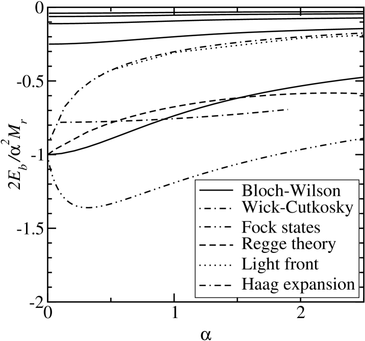
Figure 5: The binding energy $E_{b}=M-2m$ of the ground state and several excited $s$–states as a function of the “fine structure constant” $\alpha=g^{2}/(16\pi m^{2})$ for $\mu=0$, normalized to the non–relativistic ground state energy WL02 ($M_{r}=m/2$ is the reduced mass); results from the effective Schrödinger equation (8) (“Bloch–Wilson”), the ladder approximation of the Bethe–Salpeter equation (“Wick–Cutkosky”), a straightforward Fock space expansion LB01 , the leading Regge trajectory WLS01 , the Bethe–Salpeter equation in covariant light–front dynamics MC00 , and the Haag expansion GRS95 .

Solutions of Eq. (8) for some excited $s$–states are also shown. The ladder approximation of the Bethe–Salpeter equation is known in this case as the Wick–Cutkosky model, and is exactly solvable WC54 . The results from Eq. (8) lie roughly half–way between the Bethe–Salpeter and the non–relativistic results (value $(-1)$ in Fig. 5), which is reasonable in view of the results from the Feynman–Schwinger representation shown in Fig. 4.

References

- (1) Salpeter, E. E., and Bethe, H. A., Phys. Rev. 84, 1232 (1951).
- (2) Gell-Mann, M., and Low, F., Phys. Rev. 84, 350 (1951).
- (3) Nakanishi, N., Prog. Theor. Phys. (Suppl.) 43, 1 (1969).
- (4) Wick, G. C., Phys. Rev. 96, 1124 (1954); Cutkosky, R. E., Phys. Rev. 96, 1135 (1954).
- (5) Gross, F., Phys. Rev. C26, 2203 (1982).
- (6) Gross, F., Phys. Rev. 186, 1448 (1969).
- (7) Logunov, A. A., and Tavkhelidze, A. N., Nuovo Cim. 29, 380 (1963); Blankenbecler, R., and Sugar, R., Phys. Rev. 142, 1051 (1966).
- (8) Mandelzweig, V. B., and Wallace, S. J., Phys. Lett. B197, 469 (1987); Wallace, S. J., and Mandelzweig, V. B., Nucl. Phys. A503, 673 (1989).
- (9) Simonov, Yu. A., and Tjon, J. A., Ann. Phys. (N.Y.) 228, 1 (1993).
- (10) Nieuwenhuis, T., and Tjon, J. A., Phys. Rev. Lett. 77, 814 (1996).
- (11) Brodsky, S. J., Pauli, H.–C., and Pinsky, S.S., Phys. Rep. 301, 299 (1998).
- (12) Perry, R. J., and Wilson, K. G., Nucl. Phys. B403, 587 (1993).
- (13) Głazek, St. D., and Wilson, K. G., Phys. Rev. D49, 4214 (1994); Wegner, F., Ann. Phys. 3, 77 (1994); Pauli, H.–C., hep–th/9608035; Walhout, T.S., Phys. Rev. D59, 065009 (1999).
- (14) Jones, B. D., Perry, R. J., and Głazek, St. D., Phys. Rev. D55, 6561 (1997); Trittmann, U., and Pauli, H.–C., hep–th/9704215; Gubankova, E. L., Pauli, H.–C., and Wegner, F. J., hep–th/9809143.
- (15) Głazek, St., Harindranath, A., Pinsky, S., Shigemutsu, J., and Wilson, K., Phys. Rev. D47, 1599 (1993).
- (16) Weber, A., in Particles and Fields — Seventh Mexican Workshop, Ayala, A., Contreras, G., and Herrera, G., Eds., AIP Conf. Proc. No. 531 (AIP, New York, 2000).
- (17) Weber, A., and Ligterink, N. E., Phys. Rev. D65, 025009 (2002).
- (18) Wilson, K. G., Phys. Rev. D2, 1438 (1970).
- (19) Glöckle, W., and Müller, L., Phys. Rev. C23, 1183 (1981).
- (20) Ligterink, N. E., and Bakker, B. L. G., hep–ph/0010167.
- (21) Weber, A., López Vieyra, J. C., Stephens, C. R., Dilcher, S., and Hess, P. O., Int. J. Mod. Phys. A16, 4377 (2001).
- (22) Mangin–Brinet, M., and Carbonell, J., Phys. Lett. B474, 237 (2000).
- (23) Greenberg, O. W., Ray, R., and Schlumpf, F., Phys. Lett. B353, 284 (1995).