Abstract

A new approach to high energy evolution based on a linear equation for QCD generating functional is developed. This approach opens a possibility for systematic study of correlations inside targets, and, in particular, inside realistic nuclei.

Our results are presented as three new equations. The first one is a linear equation for QCD generating functional (and for scattering amplitude) that sums the ’fan’ diagrams. For the amplitude this equation is equivalent to the non-linear Balitsky-Kovchegov equation.

The second equation is a generalization of the Balitsky-Kovchegov non-linear equation to interactions with realistic nuclei. It includes a new correlation parameter which incorporates, in a model dependent way, correlations inside the nuclei.

The third equation is a non - linear equation for QCD generating functional (and for scattering amplitude) that in addition to the ’fan’ diagrams sums the Glauber-Mueller multiple rescatterings.

1 Introduction

High density QCD [1, 2, 3, 4, 5] which is a theory of Color Glass Condensate deals with parton systems with large gluon occupation numbers. It has entered a new phase of its development: a direct comparison with the experimental data. A considerable success [6, 7, 8, 9, 10, 11, 12, 13, 14, 15] has been reached in description of new precise data on deep inelastic scattering [16] as well as in understanding of general features of hadron production in ion-ion collision [17].

Most of the applications of hdQCD are based on or related to a nonlinear evolution equation derived for high density QCD [1, 2, 18, 19]. The equation sums ’fan’ diagrams, which is a subset of the semi-enhanced diagrams. In order to obtain a closed form equation it is usually assumed that color dipoles produced by the evolution interact independently [1, 19]. It was noticed in Ref. [11] that the nonlinear evolution equation based on the above assumption faces problems when applied to realistic nuclei. It was realized that in addition to multiple rescatterings on nucleons inside a nucleus we have to include in the analysis multiple rescatterings inside a single nucleon. This means a need to account for nucleus correlations. It is our motivation for this research to develop a systematic approach which would allow us to introduce correlations inside a target.

We have found that a convenient language to address the problem of target correlations is using the QCD generating functional, for which a linear evolution equation can be written. The generating functional was introduced by Mueller in Ref. [20] and then used by Kovchegov in his derivation of the non-linear evolution equation for interaction amplitude [19]. In the present paper, we show that this functional (and the amplitude) obeys a linear evolution equation involving functional derivatives with respect to initial conditions. For the linear equation we propose a systematic method to include target correlations. In general, the linear equation for the amplitude with target correlations cannot be transformed to a non-linear one. For a specific choice of correlations we are able to reduce the linear equation to a non-linear form similar to the Balitsky-Kovchegov (BK) equation. In fact, our new equation is a model dependent generalization of the BK equation for targets with correlations. It is important to stress that we consider the very same functional as of Mueller. The evolution of the dipole wave function is still based on independent production of dipoles. Only correlations for the dipole-target interaction are introduced.

Let us discuss now realistic nuclei and reasons why we believe target correlations are essential there. In principal, the BK equation is correct for hadron targets as well as for heavy nuclei. For the latter the large $A$ limit is usually assumed which adds an additional justification to the equation validity. In this case a nucleus is viewed as a very dense system of nucleons. We are going to relax this assumption. In fact the realistic nuclei are not very dense but rather dilute [10, 13]. The diluteness parameter that governs the interaction with nuclei could be expressed in the form:

$$\kappa_{A}(b)\,\,=\,\,\pi\,R^{2}_{N}\,\,S_{A}(b)\,,$$ (1.1)

where $\pi R^{2}_{N}$ is the effective area in which gluons of a nucleon are distributed. $S_{A}(b)$ stands for a nucleus profile function, which can be taken as the Wood-Saxon form factor of the nucleus.

The parameter $\kappa_{A}\,\propto\,\,A^{\frac{1}{3}}$ and , in principle, is large for heavy nuclei. It turns out, however, that the gluons are distributed inside a nucleon within a rather small area with radius of the order of $0.3-0.4fm$ [10, 13], which is much smaller compared to the proton radius. For such small area the value of $\kappa_{A}$ even for the heaviest nuclei is smaller than unity. Therefore, in spite of the pure theoretical interest to the very heavy nuclei we have to be very careful applying the large $A$ limit to the realistic nuclei. It should be stressed that even for more ‘standard’ approach with the radius of gluon distribution of the order of $0.6\,fm$ the value of $\kappa_{A}$ reaches at best 3 for heaviest nuclei. In this case the $1/\kappa_{A}$ corrections are of the order 35 % and should be accounted for when confronting with experimental data. We remind that the most interesting effects in ion-ion and hadron-ion collisions such as Cronin enhancement and $N_{part}$-scaling [17] are of the level about 25%.

In this paper we consider realistic nuclei without the large $A$ assumption. We argue that in this case a nonlinear evolution is still a valid tool. However the equation gets modified compared to the one of Ref. [19] with which our discussion will have a strong overlap. For realistic (dilute) nuclei the assumption about independent dipole interactions should be relaxed. Within some model we will be able to include correlations inside nucleus such that only one correlation factor is introduced. This factor is independent of the number of dipoles interacting with the nucleus.

The problem which we are going to deal with is very simply illustrated on the following toy example. Suppose we have a probe with two dipoles only which are close to each other on the inter-nucleon distance scale $T_{A}\,\sim A^{1/3}$. Suppose the effective interaction radius of a nucleon is $R_{N}$. Then the probability for one dipole to interact with the nucleus is $A\,R_{N}^{2}/T_{A}^{2}$. What will be the probability for two dipoles to interact with the nucleus? For the case of independent scattering it is $(A\,R_{N}^{2}/T_{A}^{2})^{2}$. It is obvious, however, that this is not what actually happens. Since the dipoles are close to each other they either both hit the nucleon or both miss it. The real probability will be rather $A\,R_{N}^{2}/T_{A}^{2}$. It follows from this discussion that the equation based on independent interactions underestimates shadowing corrections in nuclei. In the above example $\kappa_{A}\,=\,A\,R_{N}^{2}/T_{A}^{2}$.

If schematically the equation for the amplitude of Ref. [19] has the form

$$\frac{dN}{dY}\,\,=\,\,Ker\otimes\,\left[\,N\,-\,N^{2}\right]\,$$ (1.2)

then the equation which we propose for the dipole-nucleus amplitude can be written as

$$\frac{dN_{A}}{dY}\,\,=\,\,Ker\otimes\,\left[\,N_{A}\,-\,\frac{1\,+\,\kappa_{A}}{\kappa_{A}}\,N_{A}^{2}\right]\,$$ (1.3)

Eq. (1.3) can be certainly brought to the form of Eq. (1.2) provided a corresponding rescaling of the initial conditions is done. When $\kappa_{A}$ is large Eq. (1.3) reduces to Eq. (1.2). In the opposite limit $\kappa_{A}$ is small, $N_{A}\,=\,\kappa_{A}\,N_{N}$ with $N_{N}$ being a solution of Eq. (1.2) for a nucleon target.

In the final part of this paper we generalize the approach based on QCD generating functional to include Glauber-Mueller multiple rescatterings. In order to achieve our goal we construct a QCD effective vertex for one dipole splitting to many. In Pomeron language, this vertex generalizes the famous triple Pomeron vertex to the case of multiple splitting. We define a new QCD generating functional which obeys a new linear evolution equation. Without target correlations this equation can be reformulated as a new non-linear equation. In addition to the ’fan’ diagrams, the functional sums all types of semi-enhanced diagrams. We argue that in the saturation domain all semi-enhanced diagrams are of equal importance. This is why they have to be summed up in order to get a reliable description of the saturation domain. We find that the inclusion of the Glauber-Mueller multiple rescatterings leads to a significant modification of results based on ’fan’ diagrams (BK equation) only.

The structure of the paper is following. In the next section (2) we derive a linear evolution equation for generating functional and the interaction amplitude including target correlations. Section 3 is devoted to realistic nuclei. A model for nucleus correlations is proposed and a generalization of the BK equation is given. In section 4 we present a generalization of the functional approach to Glauber-Mueller multiple rescatterings. The concluding section 5 contains discussion of the results obtained.

2 Linear Equation

Though we usually consider a nonlinear evolution for the scattering amplitude it is possible to formulate the very same problem in terms of a linear functional equation. A linear formulation appears to be more suitable for treatment of correlations inside a target. We first start from a toy model which simplify the whole problem to such an extent that it could be solved analytically. Then we proceed to the complete analysis of the QCD generating functional.

2.1 A toy model

In pQCD the Pomeron is described by the linear BFKL equation [21] which is integro-differential equation. Instead we will consider a phenomenological Pomeron given by

$$\frac{d\,N(Y,\,b_{t})}{d\,Y}\,\,=\,\,\omega_{0}\,N(Y,\,b_{t})$$ (2.4)

This equation reproduces the main property of the real BFKL equation, namely, the power-like increase of the amplitude as a function of energy. So far we neglect the fact that the actual degrees of freedom are color dipoles having different sizes. We will come back to the real QCD in the next subsection.

Let $P_{n}(y)$ be a probability to find $n$-dipoles with rapidity $y$ in the wave function of the fastest (parent) dipole moving with rapidity $Y\,>\,y$. We introduce in a very simple way a probability for one dipole to decay into two:

$$K(1\,\rightarrow 2)\,\,=\,\,\omega_{0}$$ (2.5)

In (2.5) we have assumed that the triple Pomeron vertex is just $\omega_{0}\,\sim\,\alpha_{s}$. For $P_{n}(y)$ we can easily write down a reccurent equation (see Fig. 1 )

$$-\,\frac{\partial\,P_{n}(y)}{\partial\,y}\,\,=\,-\,\omega_{0}\,n\,P_{n}\,+\,\omega_{0}\,(n-1)\,P_{n-1}.$$ (2.6)

The first term in the r.h.s. can be viewed as a probability of the dipole annihilation in the rapidity range $(y\,\div\,y-dy)$. The second is a probability to create one extra dipole. Note the sign minus in front of $\partial P_{n}(y)/\partial y$. It appears due to our choice of the rapidity evolution which starts at the largest rapidity $y=Y$ of the fastest dipole and then decreases.

Figure 1: The equation for the probability to find $n$-dipoles in one fast dipole. The wave line shows a single dipole.

It is useful to introduce the generating function [22, 20, 23]

$$Z(y,\,u)\,\,=\,\,\sum_{n}\,\,P_{n}(y)\,\,u^{n}\,,$$ (2.7)

At the rapidity $y\,=\,Y$ there is only one fastest dipole, that is $P_{1}(y\,=\,Y)\,=\,1$ while $P_{n>1}(y\,=\,Y)\,=\,0$. This is the initial condition for the generating function:

$$Z(y\,=\,Y)\,=\,u\,.$$

At $u=1$

$$Z(y,\,u\,=\,1)\,\,=\,\,1$$ (2.8)

which follows from the physical meaning of $P_{n}$ as probability.

Eq. (2.6) can be rewritten as the equation in partial derivatives for the generating function $Z(y,u)$:

$$-\,\,\frac{\partial\,Z(y,\,u)}{\partial\,y}\,\,=\,\,-\,\omega_{0}\,u\,(1\,-\,u)\,\,\frac{\partial\,Z(y,\,u)}{\partial\,u}$$ (2.9)

The function $Z$ obeying Eq. (2.9) with the above given initial condition

$$Z(Y-y,\,u)\,\,=\,\,\frac{u\,\,e^{\,-\,\omega_{0}\,(Y-y)}}{1\,\,+\,\,u\,\,(e^{\,-\,\omega_{0}\,(Y\,-\,y)}\,-\,1)}\,.$$ (2.10)

It is important to observe that Eq. (2.9) can be rewritten in the nonlinear form. The general form of this equation is such that the solution to this equation is $Z(u(y))$: when $Z(u(y))$ is substituted into Eq. (2.9), the derivatives $\partial Z/\partial u$ cancel and we are left with an ordinary differential equation for $u(y)$. Using initial condition at $y\,=\,Y$ we can write

$$-\,\,\frac{\partial\,Z}{\partial\,y}|_{y=Y}\,\,=\,\,-\,\omega_{0}\,\left(\,Z\,\,-\,\,Z^{2}\,\right)|_{y=Y}\,.$$ (2.11)

Due to implicit dependence on $y$ this form will be preserved at any value of $y$. Therefore, the linear equation (see Eq. (2.9)) can be rewritten in the non-linear form:

$$-\,\,\frac{\partial\,Z(y,\,u)}{\partial\,y}\,\,=\,\,-\,\omega_{0}\left(Z\,\,-\,\,Z^{2}\right)$$ (2.12)

Eq. (2.12) coincides exactly (within the same approximation neglecting the dipole sizes) with the equation for the generating functional for the light cone dipole wave function obtained by Mueller [20]. Eq. (2.9) can be viewed as a linearized version of the non-linear Eq. (2.11).

To find the interaction amplitude we can follow the procedure suggested in Ref.[19], namely,

$$N_{A}(y,\,b_{t})\,\,=\,\,Im\,A^{el}(y,\,b_{t})\,\,=\,\,-\sum^{\infty}_{n=1}\,\,\frac{1}{n!}\,\,\frac{\partial^{n}Z}{(\partial u)^{n}}|_{u=1}\,\,\gamma^{n}(b_{t})\,.$$ (2.13)

Here $\gamma(b_{t})$ is minus imaginary part of the elastic amplitude for a single dipole interaction with a nucleus at fixed impact parameter $b_{t}$. The most important assumption made in Eq. (2.13) is in the independent interaction of $n$ dipoles which is expressed via $\gamma^{n}$ factor. In the present work we will relax this assumption introducing target correlations. Note that the amplitude $N_{A}$ can be found from the following relation

$$N_{A}(y,\,b_{t})\,\,=\,\,1\,\,-\,\,Z(y,\,\gamma(b_{t})\,+\,1)\,.$$ (2.14)

Let us now come back to Eq. (2.9) from which we are going to derive a corresponding equation for the amplitude $N_{A}$. In order to get a closed equation, the linear Eq. (2.9) is differentiated $n$ times with respect to $u$ and then set $u=1$:

$$-\,\frac{1}{\omega_{0}}\,\frac{\partial\,Z^{(n)}}{\partial\,y}|_{u=1}\,\,=\,\,n\,\,Z^{(n)}|_{u=1}\,\,+\,2\,\frac{n\,(n-1)}{2}\,\,Z^{(n-1)}|_{u=1}$$ (2.15)

where $Z^{(n)}\,\,=\,\,\partial^{n}\,Z/\partial\,u^{n}$.

The equation for the amplitude can be easily obtained from Eq. (2.15). The following four operations are performed. i) Since $Z$ is a function of $Y\,-\,y$, we make a substitution $\partial Z^{n}/\partial y\,=\,-\,\partial Z^{n}/\partial Y$. Hence the amplitude evolution will be with respect to initial rapidity of the fastest dipole $Y$. (ii) At the rapidity of the target $y\,=\,y_{0}$ initial conditions for the interaction of the ’wee’ dipoles with the target should be specified. (iii) For independent interactions with the target (ii) means we multiply Eq. (2.15) by the factor $\gamma^{n}$. (iv) Divide both sides by $n!$ and then sum over $n$. The result is

$$\frac{1}{\omega_{0}}\,\frac{\partial\,N_{A}(Y)}{\partial\,Y}\,\,=\,\,\gamma\,\frac{\partial\,N_{A}(Y,\;\gamma)}{\partial\,\gamma}\,\,+\,\,\gamma^{2}\,\,\frac{\partial\,N_{A}(Y,\;\gamma)}{\partial\,\gamma}$$ (2.16)

Eq. (2.16) can be rewritten in the non-linear form using the initial condition $N_{A}(Y\,=\,y_{0})\,=\,-\,\gamma$:

$$\frac{1}{\omega_{0}}\,\frac{\partial\,N_{A}(Y)}{\partial\,Y}\,\,=\,\,N_{A}(Y)\,\,-\,\,N_{A}^{2}(Y)$$ (2.17)

Eq. (2.17) is just the BK non-linear equation [18, 19] in our simplified model.

Let us now discuss a way the target correlations can be introduced in the analysis. For the linear evolution they appear when we specify in the initial conditions how $n$ ’wee’ dipoles interact with the target. An appropriate modification is to introduce correlation factors $C_{n}$ such that

$$N_{A}(y,\,b)\,\,=\,\,-\,\,\sum^{\infty}_{n=1}\,\,\frac{1}{n!}\,\,\frac{\partial^{n}\,Z}{\partial\,u^{n}}|_{u=1}\,\,\,\gamma^{n}\,\,\,C_{n}\,.$$ (2.18)

The coefficients $C_{n}$ are to be found from a nucleus model. The linear equation for the amplitude now reads

$$\frac{1}{\omega_{0}}\,\frac{\partial\,N_{A}(Y)}{\partial\,Y}\,\,=\,\,\gamma\,\frac{\partial\,N_{A}(Y,\;\gamma)}{\partial\,\gamma}\,\,+\,\,F\left(\gamma\,\frac{\partial}{\partial\,\gamma}\right)\,\,\gamma^{2}\,\,\frac{\partial\,N_{A}(Y,\;\gamma)}{\partial\,\gamma}$$ (2.19)

Where function $F$ is equal to $F(n)\,=\,C_{n}/C_{n-1}$ and describes correlations in the interactions of $n$ dipoles. In Eq. (2.19), $F(\gamma\,\frac{\partial}{\partial\,\gamma})$ should be understood as operator series expansion. In case $F$ is constant the linear equation (2.19) reads

$$\frac{1}{\omega_{0}}\,\frac{\partial\,N_{A}(Y)}{\partial\,Y}\,\,=\,\,\gamma\,\frac{\partial\,N_{A}(Y,\;\gamma)}{\partial\,\gamma}\,\,+\,\,F\,\,\gamma^{2}\,\,\frac{\partial\,N(Y)}{\partial\,\gamma}$$ (2.20)

At $Y\,=\,y_{0}$ the initial condition is $N(Y\,=\,y_{0})\,=\,-\,C_{0}\,\gamma$. It is used to obtain from Eq. (2.20) the non-linear equation:

$$\frac{1}{\omega_{0}}\,\,\frac{\partial\,N_{A}}{\partial\,Y}\,\,=\,\,N_{A}(Y)\,\,-\,\,K_{A}\,N_{A}^{2}(Y)\,.$$ (2.21)

with $K_{A}\,=\,F/C_{0}$. In fully non-correlated case $F\,=\,C_{0}\,=\,1$, Eq. (2.21) reduces to the BK equation for the above toy model. In the next section we will consider realistic nuclei for which correlations can be modeled. We will show that within certain assumptions the correlation factor $K_{A}$ is indeed a constant but different from unity. It is important to stress that Eq. (2.20) can be brought to a nonlinear form for constant $F$ only. Otherwise $N_{A}$ is not a function of a single variable $\gamma(Y)$ and Eq. (2.20) is a linear equation involving high orders of partial derivatives.

The success of the simple toy model considered above leaves us with two hopes for real QCD dynamics. First, we believe in a possibility to find a linear functional equation for the generating functional. A linear equation is more transparent and more feasible to solve compared to the non-linear one. Second, we believe that Eq. (2.21) (generalized to include BFKL kernel) is the correct generalization of the BK non-linear equation applicable to targets with correlations such as realistic nuclei.

It turns out that a generalization of a linear functional approach to evolution kernels but simplified to a double log accuracy is rather straightforward [23]. For the complete BFKL kernel, however, this is a nontrivial problem with which we will deal below.

2.2 QCD generating functional for ’fan’ diagrams

In this subsection we consider a linear generating functional for ’fan’ diagrams in QCD. We include both the LO BFKL evolution of the dipole wave function and QCD triple Pomeron vertex (in large $N_{c}$ approximation). Then we essentially repeat the same derivation as for the toy model above. For simplicity of presentation we will not treat the impact parameter ($b_{t}$) dependencies in a correct way which would imply taking care of all relevant shifts in $b_{t}$. Instead, we will consider $b_{t}$ just as an external parameter which often will not be written explicitly. It should be of no problem to reconstruct a correct $b_{t}$ dependencies in the final results.

As in Ref. [20] we introduce a generating functional $Z$

$$Z\left(Y-y,\,r,\,b_{t};\,[u]\right)\,\,\equiv\,\,\sum_{n=1}\,\int\,\,P_{n}\left(Y-y,\,r,\,b_{t};\,r_{1},\,r_{2},\dots,r_{i}\,\dots,r_{n}\right)\,\,\prod^{n}_{i=1}\,u(\vec{r}_{i})\,d^{2}\,r_{i}$$ (2.22)

where $u(\vec{r}_{i})\equiv u_{i}$ is an arbitrary function of $r_{i}$. $P_{n}$ stands for a probability density to find $n$ dipoles with transverse sizes $r_{1},\,r_{2},\dots,\,r_{i}\,\dots\,r_{n}$ and rapidity $y$ in the wave function of the fast moving dipole of the size $r$ and rapidity $Y\,>\,y$. Note that contrary to Refs. [20, 19] we define $P_{n}$ as a dimensionful quantity. The functional (2.22) obeys two conditions:

• At $y\,=\,Y$,   $P_{n=1}\,=\,\delta^{2}(\vec{r}\,-\,\vec{r}_{1})$ while $P_{n>1}\,=\,0$. In other words,

  $$Z\left(Y\,-\,y\,=\,0,\,r,\,b_{t};\,[u]\right)\,\,=\,\,u(r)\,\,.$$ (2.23)

• At $u\,=\,1$

  $$Z\left(Y\,-\,y,\,r,\,b_{t};\,[u=1]\right)\,\,=\,\,1\,.$$ (2.24)

  This equation follows from the physical meaning of the functional: sum over all probabilities equals one.

Contrary to the toy model, in QCD the probability to survive for a dipole of size $r_{i}$ is not constant but equal to (see Ref. [20] for details)

$$\bar{\alpha}_{s}\,\,\omega(r_{i})\,\,=\,\,\frac{\bar{\alpha}_{s}}{2\,\pi}\,\int_{\rho}\,\frac{r_{i}^{2}}{(\vec{r_{i}}\,-\,\vec{r}^{\prime})^{2}\,r^{\prime 2}}\,d^{2}r^{\prime}\,\,=\,\,\bar{\alpha}_{s}\,\,\ln(r_{i}^{2}/\rho^{2})$$

with $\rho$ being some infrared cutoff and $\bar{\alpha}_{S}\,=\,\alpha_{S}\,N_{c}/\pi$. The probability for a dipole of the size $r_{1}\,+\,r_{2}$ to decay into two with the sizes $r_{1}$ and $r_{2}$ is equal to

$$\frac{\bar{\alpha}_{s}}{2\,\pi}\,\,\frac{(\vec{r_{1}}\,\,+\,\,\vec{r_{2}})^{2}}{r_{1}^{2}\,r_{2}^{2}}$$

Using these two probabilities we can write down the equation for $P_{n}$:

$$-\,\,\frac{\partial\,P_{n}\left(Y-y,\,r,\,b_{t};\,r_{1},\,r_{2}\dots r_{i}\dots r_{n}\right)}{\bar{\alpha}_{s}\,\partial\,y}\,=\,-\,\sum^{n}_{i=1}\,\omega(r_{i})\,P_{n}\left(Y-y,\,r,\,b_{t};\,r_{1},\,r_{2}\dots r_{i}\dots r_{n}\right)$$

$$+\,\,\sum^{n}_{i=1}\,\frac{(\vec{r}_{i}\,+\,\vec{r}_{n})^{2}}{(2\,\pi)\,r^{2}_{i}\,r^{2}_{n}}\,P_{n-1}\left(Y-y,\,r,\,b_{t};\,r_{1},\,r_{2}\dots(\vec{r}_{i}\,+\,\vec{r}_{n})\dots r_{n-1}\right)$$ (2.25)

Let us now introduce two operator vertices

$$V_{1\rightarrow 1}(r,\,[u])\,\,=\,\,\bar{\alpha}_{s}\,\,\omega(r)\,\,u(\vec{r})\,\,\frac{\delta}{\delta u(\vec{r})}$$ (2.26)

and

$$V_{1\rightarrow 2}(r,\,r^{\prime},\,[u])\,\,=\,\,\frac{\bar{\alpha}_{s}}{2\,\pi}\,\,\frac{r^{2}}{r^{\prime 2}\,(\vec{r}-\vec{r}^{\prime})^{2}}\,\,\,u(\vec{r}^{\prime})\,u(\vec{r}\,-\,\vec{r}^{\prime})\,\,\frac{\delta}{\delta u(\vec{r})}\,.$$ (2.27)

The functional derivatives with respect to $u(r)$ play a role of an annihilation operator for a dipole of the size $r$. The multiplication by $u(r)$ corresponds to a creation operator for this dipole.

Multiplying Eq. (2.2) by the product $\prod^{n}_{i=1}\,u_{i}$ and integrating over all $r_{i}$ we obtain the following linear equation for the generating functional:

$$-\,\,\frac{\partial\,Z}{\bar{\alpha}_{s}\,\partial\,y}\,\,=\,\,-\,\,\int\,d^{2}r^{\prime}\,\,V_{1\rightarrow 1}(r^{\prime},\,[u])\,\,Z\,\,+\,\,\int\,\,d^{2}\,r^{\prime\prime}\,\,d^{2}\,r^{\prime}\,\,V_{1\rightarrow 2}(r^{\prime\prime},\,r^{\prime},\,[u])\,\,Z\,.$$ (2.28)

Like in the case of previously considered toy model, $Z$ is a function of a single variable $u(y)$: if $Z(u(y))$ is substituted into Eq. (2.28) we find in the l.h.s. $\partial\,Z/\partial\,y\,=\,\int d^{2}r\,(\delta Z/\delta\,u(r))\,\,(\partial\,u(r)/\partial\,y)$. The integrals $\int d^{2}r\,\delta Z/\delta\,u(r)$ cancel on both sides of the equation and we are left with an ordinary differential equation for $u(y)$. With the help of the initial conditions (Eq. (2.23)), Eq. (2.28) can be rewritten in the non-linear form reproducing the same equation for $Z$ as in Ref. [20]:

$$-\,\,\frac{\partial\,Z}{\bar{\alpha}_{s}\,\partial\,y}\,\,=\,\,-\,\,\omega(r)\,\,Z\left(Y\,-\,y,\,r,\,b_{t};\,[u]\right)$$ (2.29)

$$+\,\,\int\,\,\frac{d^{2}\,r^{\prime}}{2\,\pi}\,\,\frac{r^{2}}{r^{\prime 2}\,(\vec{r}\,-\,\vec{r}^{\prime})^{2}}\,\,Z\left(Y\,-\,y,\,r^{\prime},\,b_{t};\,[u]\right)\,\,Z\left(Y\,-\,y,\,(\vec{r}\,-\,\vec{r}^{\prime}),\,b_{t};\,[u]\right)\,.$$

The amplitude $N_{A}$ is defined similarly to Eq. (2.13) (see Ref. [19]):

$$N_{A}(Y,\,r,\,b_{t})\,\,=\,\,-\,\,\sum^{\infty}_{n=1}\,\,\frac{1}{n!}\,\,C_{n}\,\,\int\,\prod^{n}_{i=1}\,\,\left(d^{2}\,r_{i}\,\,\gamma(r_{i};b_{t})\,\,\frac{\delta}{\delta u_{i}}\right)\,Z\left(Y-y,\,r,\,b_{t};\,[u]\right)|_{u=1}.$$ (2.30)

As above $C_{n}$ describe correlations in the $n$-dipole target interaction. In order to derive an expression for the amplitude $N_{A}$ we apply to both sides of Eq. (2.29) $n$ functional derivatives with respect to $u$ and then set $u=1$. Using the notation $Z^{(n)}\,\,\equiv\,\,\prod^{n}_{i=1}\frac{\delta}{\delta u_{i}}\,Z\left(Y-y,\,r,\,b_{t};\,[u]\right)$ we obtain

$$-\,\frac{\partial}{\bar{\alpha}_{s}\,\partial\,y}\,Z^{(n)}|_{u=1}\,\,=\,\,\left(-\,\sum_{i=1}^{n}\,\,\omega(r_{i})\,\,Z^{(n)}|_{u=1}\,\,\,+\,\,2\,\sum_{i=1}^{n}\,\int\,\frac{d^{2}\,r^{\prime}}{2\,\pi}\,\,\frac{r^{\prime 2}}{r^{2}_{i}\,(\vec{r}_{i}\,-\,\vec{r}^{\prime})^{2}}\,\,Z^{(n)}|_{u=1}\,\,\right.$$

$$\left.+\,\,\sum_{i,\,j=1;\,j\neq i}^{n}\,\frac{(\vec{r}_{i}+\vec{r}_{j})^{2}}{(2\,\pi)\,r^{2}_{i}\,r^{2}_{j}}\,\,Z^{(n)}|_{u=1}\,\right)\,.$$ (2.31)

The evolution equation for the amplitude is obtained through the same steps as in the toy model above. We divide Eq. (2.31) by $n!$ and multiply by the product $-\,C_{n}\,\prod^{n}_{i=1}\,\gamma(r_{i},\,b_{t})$. Then we integrate over all $r_{i}$ and sum over $n$. Finally we consider the evolution with respect to $Y$ instead of $y$ which implies a change of sign in front of the derivative:

$$\frac{\partial\,N_{A}(Y;\,[\gamma])}{\bar{\alpha}_{s}\,\partial\,\,Y}\,\,=\,\,-\int\,d^{2}\,r^{\prime}\,\,V_{1\rightarrow 1}(r^{\prime},\,[\gamma(r^{\prime})])\,\,N_{A}(Y;\,[\gamma])\,\,$$ (2.32)

$$+\,\,\frac{2}{2\,\pi}\,\int\,d^{2}\,r^{\prime}\,d^{2}\,r"\,\,\gamma(r")\,\frac{r^{\prime 2}}{\,r"^{2}\,(\vec{r}"\,-\,\vec{r}^{\prime})^{2}}\,\,\frac{\delta}{\delta\,\gamma(r^{\prime})}\,\,N_{A}(Y;\,[\gamma])$$

$$+\,\,F\left(\int\,d^{2}\,\bar{r}\,\gamma(\bar{r})\,\frac{\delta}{\delta\gamma(\bar{r})}\right)\,\,\int\,d^{2}\,r"\,\,d^{2}\,r^{\prime}\,\,V_{1\rightarrow 2}(r^{\prime},\,r",\,[\gamma(r^{\prime})])\,\,N_{A}(Y;\,[\gamma])$$

Eq. (2.32) is linear but in functional derivatives and it is not easy to develop direct methods to solve it. In case of function $F$ being a constant, Eq. (2.32) can be easily reduced to a non-linear equation. Using the initial condition $N_{A}(Y\,=\,y_{0})\,=\,-\,C_{0}\,\gamma$ we obtain the following nonlinear equation:

$$\frac{\partial\,N_{A}(r,\,y;\,b_{t})}{\partial\,Y}\,=\,\bar{\alpha}_{S}\,\times\int_{\rho}\,\frac{d^{2}\,r^{\prime}}{2\,\pi}\,\frac{r^{2}}{r^{\prime 2}\,(\vec{r}\,-\,\vec{r}^{\prime})^{2}}\,\,\times$$ (2.33)

$$\left[\,2\,N_{A}(r^{\prime},\,y;\,b_{t})\,\,-\,\,N_{A}(r,\,y;\,b_{t})\,\,-\,\,K_{A}\,\,N_{A}(r^{\prime},\,y;\,b_{t})\,\,N_{A}(\vec{r}\,-\,\vec{r}^{\prime},\,y;\,b_{t})\right]\,,$$

with $K_{A}\,\equiv\,F/C_{0}$. If we consider dipole interaction as fully uncorrelated $F\,=\,C_{0}\,=\,1$ then Eq. (2.33) reduces to the BK equation. We will find below that within some assumptions, correlations in realistic nuclei can be described by a constant $F$, but with $F\,\neq\,C_{0}$. In this case Eq. (2.33) is a generalization of the BK equation to realistic nuclei with correlations.

3 Dipole-nucleus interactions with correlations

3.1 Nucleus correlations

Let us discuss the target correlations starting with dipole-nucleus interactions at sufficiently low energy ($y_{0}=\,\ln(1/x_{0})$). It should be stressed that the energy is supposed to be not too low such that high energy QCD is applicable. On the other hand, we assume that energy is low enough such that a single dipole interacts with one nucleon only. We neglect all Glauber rescatterings at this energy.

Consider first the Fig. 2 which presents in details how a single dipole interacts with a nucleus. Schematically the same is displayed in (Fig. 3-a).

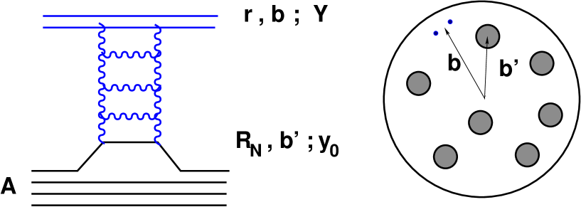
Figure 2: The exchange of the single BFKL Pomeron for dipole-nucleus scattering.

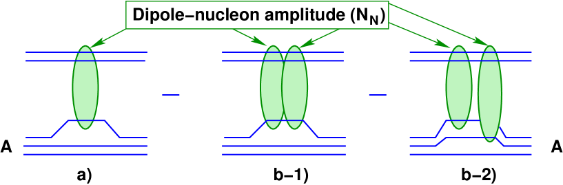
Figure 3: A single dipole and two dipole nucleus amplitudes.

Its contribution is proportional to $\kappa_{A}(b_{t})$:

$$\int d^{2}b^{\prime}\,N_{N}(r,\,y_{0};\,\vec{b}_{t}\,-\,\vec{b}_{t}^{\prime})\,S_{A}(b_{t}^{\prime})\,=\,S_{A}(b_{t})\,\int d^{2}b_{t}"\,N_{N}(r,\,y_{0};\,b_{t}")\,\approx\,\,N_{N}(r,\,y_{0};\,b_{t}=0)\,\kappa_{A}(b_{t})\,.$$ (3.34)

Here $N_{N}$ stands for the imaginary part of the dipole-nucleon elastic amplitude. $N_{N}$ can, in principal, include multiple dipole-nucleon rescatterings. As it is clear from Eq. (3.34) and Fig. 2 that $b_{t}$ is a distance from the nucleus center to a given nucleon.

In Eq. (3.34) the first equality is due to the assumption, standard for the Glauber theory, that the size of the nucleon as well as the radius of the dipole-nucleon interaction is much smaller than the size of the nucleus. The second equality is model dependent. We have assumed a cylindrical nucleon that is $N_{N}(r,\,y_{0};\,b_{t})\,=\,N_{N}(r,\,y_{0};\,b_{t}=0)\,\,\Theta(R_{N}\,-\,b_{t})$. The parameter $\kappa_{A}(b_{t})$ (Eq. (1.1)) measures the strength of the dipole nucleus interaction.

Consider now diagrams of Fig. 3-b. For very large nuclei the diagram of Fig. 3-b-2 dominates since it is proportional to $\kappa^{2}_{A}(b_{t})$ while the diagram of Fig. 3-b-1 is of the order $\kappa_{A}(b_{t})$ only. In the case when $\kappa_{A}(b_{t})$ is not large the diagram of Fig. 3-b-1 should be also taken into account. Its contribution has the form:

$$-\,\int\,\,d^{2}\,b_{t}^{\prime}\,\left(N_{N}(r,y_{0};\vec{b}_{t}-\vec{b}_{t}^{\prime})\right)^{2}\,S_{A}(b_{t}^{\prime})\,\,\simeq\,\,\left(N_{N}(r,\,y_{0};\,b_{t}\,=\,0)\right)^{2}\,\,\kappa_{A}(b_{t})\,.$$ (3.35)

Fig. 3-b should be viewed as interaction of two dipoles with the nucleus. Fig. 3-b-1 is a correlated interaction with one and the same nucleon while Fig. 3-b-2 is independent interaction with different nucleons. In Eq. (3.35) we have neglected the difference in the dipole sizes, which is not important for this discussion.

If we proceed further for higher order terms we can find a general expression for $n$-th term in the expansion. For three dipoles we have a term proportional to $\kappa_{A}$ when all three interact with the same nucleon, a term proportional to $\kappa_{A}^{2}$ when two dipoles are correlated, and a term proportional to $\kappa_{A}^{3}$ when all interact independently. The sum of these terms will be

$$N_{N}^{3}\,\,(\kappa_{A}\,+\,2\,\kappa_{A}^{2}\,+\,\kappa_{A}^{3})\,.$$

The factor 2 in front of $\kappa_{A}^{2}$ is due to combinatorial counting. The $n$-th term in the expansion has the form:

$$(-1)^{n}\,\,\kappa_{A}\,(1\,+\,\kappa_{A})^{n-1}\,\,N_{N}^{n}\,.$$ (3.36)

There is no time ordering associated with the factor $1/n!$ which usually appears in the Galuber expansion. $(-1)^{n}$ stems from the fact that the dipole-nucleon amplitude at $y_{0}\,=\,\ln(1/x_{0})\,\gg\,1$ is pure imaginary.

From Eq. (3.36) we can read off the correlation coefficients $C_{n}$ introduced above: $C_{n}\,=\,\kappa_{A}\,(1\,+\,\kappa_{A})^{n-1}$. Hence the correlation function $F\,=\,(1\,+\,\kappa_{A})$ and the correlation parameter $K_{A}\,=\,(1\,+\,\kappa_{A})/\kappa_{A}$. The correlations appeared when the assumption about independent interactions was relaxed. In spite of the introduction of the correlation parameter, Eq. (3.36) still allow interpretation in terms of independent dipole-nucleus interactions. The strength of this interaction is $(1\,+\,\kappa_{A})\,N_{N}$. In fact the dipoles interact ’almost’ independently and only the overall factor $\kappa_{A}/(1+\kappa_{A})$ incorporates the correlations inside the nucleus. The most important fact is that we were able to introduce only one correlation parameter independent of the number of dipoles participating in the interaction. This success can be traced back to the model assumption about the cylindricity of nucleons.

3.2 Nonlinear equation for realistic nuclei

Above we have considered correlated interactions of $n$-dipoles with a realistic (relatively dilute) nucleus. We have found the correlation factor $K_{A}\,=\,(1\,+\,\kappa_{A})/\kappa_{A}$ which is to be substituted into Eq. (2.33). As a result, Eq. (2.33) gives a generalization of the BK equation to realistic nuclei with correlations. As was already mentioned in the introduction, Eq. (2.21) respects both small and large limits of $\kappa_{A}$. It is most important to stress that the correlation factor $K_{A}$ is always $\gg\,1$. This means the nucleus correlations increase the shadowing. In other words, the BK equation which assumes independent interactions underestimates shadowing corrections for realistic nuclei.

Let us now present some numerical estimates related to Eq. (2.21). The effective nucleon radius found in Ref. [10] is $R_{N}^{2}\,=\,3.1\,GeV^{2}$. At zero impact parameter $b_{t}\,=\,0$, $\kappa_{A}(b_{t})$ is maximal. For the heaviest nuclei, say gold ($A=197$), $\kappa_{Au}(0)\,\simeq\,0.85$ while for neon ($A=20$) $\kappa_{Ne}(0)\,\simeq\,0.35$.

In the deep saturation region a solution of Eq. (2.21) will saturate. The saturation bound will not be unity but $N_{A}\,=\,1/K_{A}\,\leq\,1$. In order to confirm our expectations Eq. (2.21) is solved numerically for gold nucleus at $b_{t}\,=\,0$ (Fig. 4).

Figure 4: The solution of Eq. (2.21) as a function of $r$ for $b_{t}\,=\,0$.

The initial conditions are set at $x\,=\,x_{0}\,=10^{-2}$. Consistently with our derivation we take $N_{A}(x_{0},\,r)\,=\,\kappa_{A}(0)\,N_{N}(x_{0},\,r)$ with $N_{N}$ being a dipole nucleon amplitude found in Ref. [10]. The function $N_{A}$ shown in Fig. 4 indeed saturates at the value $1/K_{A}$ in accord with the expectations.

3.3 Non-linear equation and enhanced diagrams

.

The BK nonlinear evolution equation sums the ’fan’ diagrams of Fig. 5-1. It is important to understand the limits of its applicability and develop methods to include necessary corrections. Two types of diagrams which are not included in the BK equation are show in Fig. 5-2 and Fig. 5-3. These are semi-enhanced diagrams including multiple Pomeron vertices (Fig. 5-2) and the enhanced diagram with Pomeron loops.

The diagram of Fig. 5-2 can be neglected in pre-saturation region only, when $N_{A}\ll 1$. Thus, in spite of its importance to high energy phenomenology, the validity of the BK equation is limited to $r\,<\,1/Q_{s}$. In the next section we will propose a new non-linear equation, which is supposed to sum the ’fan’ diagrams as well as those of Fig. 5-2.

The assumption of large $\kappa_{A}\,\gg\,1$ was essential in arguments given in Ref. [19] in order to neglect the enhanced diagrams of Fig. 5-3. Indeed, the ’fan’ diagrams dominate in this limit [24]. As we have argued above, for realistic nuclei $\kappa_{A}\,\leq\,1$ and the argument is not applicable. Nevertheless we are still convinced that the Pomeron loop diagrams are subleading provided the projectile dipole has a small size.

Following Refs. [1, 2, 3] we can estimate a contribution of the enhanced diagram of Fig. 5-3. The ladders are associated with the BFKL Pomeron having the property discussed earlier:

$$N\,\,\propto\,\,e^{\omega_{0}\,y}$$ (3.37)

with $\omega_{0}\,\propto\,\alpha_{s}$. The integration over $y_{1}$ and $y_{2}$ leads to

$$N^{enhanced}_{A}\,\,\,\,\propto\,\,\,\,\frac{1}{\omega_{0}(r)\,\,\omega_{0}(R)}\,\,\,e^{\,2\,\,\omega_{0}\,(Y\,-\,0)}\,\,\approx\,\,\frac{1}{\alpha_{s}(r)\,\alpha_{s}(R)}\,\,e^{2\,\,\omega_{0}\,Y}\,.$$ (3.38)

The typical values of $Y-y_{1}\,\approx\,1/\omega(r)\,\,\gg\,1$ while $y_{2}-0\,\,\approx\,\,1/\omega(R)\,\,\,\approx\,\,1$. Therefore, the upper ladder which is in the region where the QCD coupling is small, describes a high energy process for which the BFKL equation can be trusted. On the other hand, the lowest ladder corresponds to the interaction at rather low energies where high energy asymptotic expressions are not applicable. Consequently, the enhanced diagram of Fig. 5-3 should be viewed as degenerate with the ’fan’ diagram of Fig. 5-1. A more accurate estimate of Fig. 5-3 involves integrations over dipole sizes in the vertices but they do not alter the conclusion (see Refs. [1, 2] for details). The argument above depends crucially on the running QCD coupling and the fact that $\alpha_{s}(r)\,\ll\,\alpha_{s}(R)$. Concluding we expect the equation summing ’fan’ diagrams only be justified for nucleon targets if the projectile dipole $r$ is small, such that $\alpha_{s}(r)\,\ll\,1$.

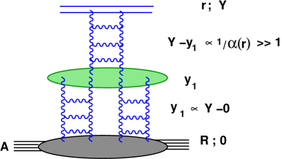
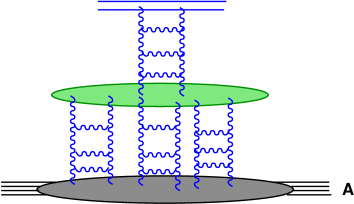
Fig. 5-1	Fig. 5-2
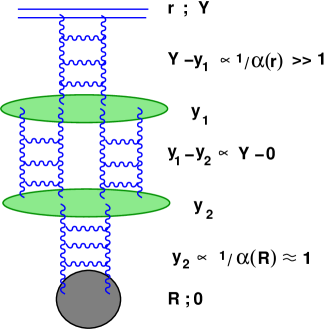
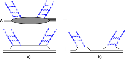
Fig. 5-3	Fig. 5-4

Figure 5: The ’fan’ diagrams (Fig. 5-1 and Fig. 5-2) for dipole-nucleus interaction. First enhanced diagram (Fig. 5-3). Fig. 5-4 shows a model for the interaction of the BFKL Pomeron with nucleus target.

It is worth to emphasize that even the ‘fan’ diagram contribution depends on the model for the ‘two ladders-nucleus’ vertex (see Fig. 5-1). In this paper we have assumed a model which graphically is represented in Fig. 5-4. This model includes the eikonal-type of interaction with the nucleon.

4 Glauber rescattering and QCD generating functional

As was discussed above, Eq. (2.28) for generating functional, which is equivalent to the one obtained by Mueller, describes the ’fan’ diagrams only. The fact that this equation does not describe the semi-enhanced diagrams of the type shown in Fig. 5-2 is an apparent shortcoming. At dipole sizes $r\,\geq\,R_{s}(x)\,=\,2/Q_{s}(x)$ these diagrams are of the same order as the ’fan’ diagrams and they have to be taken into account in order to obtain a reliable description of the saturation domain. In this section we propose a generalization of the QCD functional approach to such type of interactions. To simplify the presentation we will not consider target correlations in this section.

In order to solve the problem we have to find an effective vertex for one dipole splitting to many. This vertex can be deduced from the Glauber-Mueller formula [25, 26, 27] which describes propagation of a dipole through large nucleus. It is important to stress that this formula was proven in QCD. In our approach, the effective vertex will be obtained as a chain of multiple rescatterings involving a dipole splitting to two dipoles.

The Glauber-Mueller formula reads

$$N^{GM}(y,\,r,\,b_{t})\,\,=\,\,\left(\,1\,\,-\,\,e^{-N^{BFKL}(y,\,r,\,b_{t})}\,\right)$$ (4.39)

with $N^{BFKL}$ being a solution to the linear BFKL equation. We can use Eq. (4.39) to define initial conditions for a new functional. $N^{BFKL}$ describes a single Pomeron exchange which in the language of section 2 should be replace by $1\,-\,u$. Basing on the relation Eq. (2.14) we propose the following initial conditions at $y\,=\,Y$:

$$Z\left(Y-y\,=\,0,\,r,\,b_{t};\,[u]\right)\,\,=\,\,e^{u(r)\,-\,1}\,\,.$$ (4.40)

At $u\,=\,1\,\,$, $\,Z$ has the correct normalization: $Z\,=\,1$.

Eq. (4.40) can be given the following interpretation. Contrary to the case considered in section 2 where we had a single dipole at the beginning of the evolution, Eq. (4.40) describes initial state in which many dipoles can be created. $Z$ represents a probability distribution for a dipole number in the initial state. It can be rewritten as

$$Z\left(Y\,=\,y,\,r,\,b_{t};\,[u]\right)\,=\,\sum_{n=0}e^{\,-\,<n>}\,\frac{(u\,<n>)^{n}}{n!}$$ (4.41)

The average number of dipoles $<n>\,\equiv\,\frac{\delta}{\delta\,u}Z|_{u=1}\,=\,1$. Eq. (4.41) is a typical Poisson distribution with $e^{\,-\,<n>}\,<n>^{n}/n!\,=\,e^{-1}/n!$ being a probability to find $n$ dipoles (of the same size) in the initial state.

As in section 2, the overall probability conservation implies that at $u\,=\,1$

$$Z\left(Y-y,\,r,\,b_{t};\,[u=1]\right)\,\,=\,\,1\,$$ (4.42)

to be fulfilled at any rapidity.

We are going now to find a new effective vertex $\mathcal{V}$ for one dipole splitting to many. The strategy is following. We consider a two step process. First, a dipole of size $\vec{r}$ decays into two dipoles of sizes $\vec{r}^{\prime}$ and $\vec{r}\,-\,\vec{r}^{\prime}$. This process is described by the vertex $V_{1\rightarrow 2}$ introduced in Eq. (2.27). Then each produced dipole is considered not as a single dipole but rather having a Poisson distributed dipole multiplicity of equal size dipoles. This step is described using the Glauber - Mueller formula.

The amplitude $\tilde{N}$ for this two step propagation can be written in the form [27]

$$\frac{\partial\,\tilde{N}(y,\,r)}{\partial y}\,\,=\,\,-\,\,\bar{\alpha}_{s}\,\,\omega(r)\,\,\left(1\,-\,e^{\,-\,N^{BFKL}(y,\,r)}\right)\,\,+$$ (4.43)

$$\,\,\frac{\bar{\alpha}_{s}}{2\,\pi}\,\,\int\,\frac{r^{2}\,d^{2}r^{\prime}}{r^{\prime 2}\,(\vec{r}\,-\,\vec{r}^{\prime})^{2}}\,\left(1\,\,-\,\,e^{\,-\,\{N^{BFKL}(y,\,r^{\prime})\,\,+\,\,N^{BFKL}(y,\vec{r}\,-\,\vec{r}^{\prime})\,\}}\right)\,.$$

The first term in Eq. (4.43) is a possibility for the parent dipole ($r$) not to decay while the second term describes the decay. The probability for this decay is given by the square of the wave function $|\Psi|^{2}\,=\,\bar{\alpha}_{s}\,\frac{r^{2}}{r^{\prime 2}\,(\vec{r}-\vec{r}^{\prime})^{2}}$. Two fast dipoles thus created then percolate through the target preserving their sizes. This process is described by Eq. (4.43).

It is important to explain the difference between Eq. (4.39) and Eq. (4.43). Eq. (4.39) describes a propagation of a dipole with the size $r$ through target without decay. Alternative it can be viewed as including decays but with decay products being identical dipoles with the same size and rapidity. On the other hand, Eq. (4.43) describes the two stage process. The physics of Eq. (4.43) could be clarified if we rewrite it in the following form

$$\frac{\partial\,\tilde{N}(y,\,r)}{\partial y}\,\,=\,\,-\bar{\alpha}_{s}\,\omega(r)\,N^{GM}(y,\,r)\,\,+\,\,$$ (4.44)

$$\frac{\bar{\alpha}_{s}}{2\,\pi}\,\,\int\,\frac{r^{2}\,d^{2}r^{\prime}}{r^{\prime 2}\,(\vec{r}\,-\,\vec{r}^{\prime})^{2}}\,\,\left(\,N^{GM}(y,\,r^{\prime})\,\,+\,\,N^{GM}(y,\,\vec{r}\,-\,\vec{r}^{\prime})\,\,-\,\,N^{GM}(y,\,r^{\prime})\,\,N^{GM}(y,\,\vec{r}\,-\,\vec{r}^{\prime})\right)\,.$$

We would like to emphasize that the splitting kernel is the same LO BFKL kernel as appears in the BK equation.

We are now in the position to extract from Eq. (4.43) an effective vertex $\mathcal{V}$. We interpret the Glauber- Mueller formula as an annihilation of a scattering dipole and a creation of a number of identical new dipoles. Basing on our previous experience in section 2 we substitute in the r.h.s. of Eq. (4.43) $1\,-\,u$ instead of $N^{BFKL}$ (see Eq. (2.13) and Ref.[19]) and obtain the generalized vertex

$$\mathcal{V}(r;\,[u])\,\,=\,\,\bar{\alpha}_{s}\,\left(-\,\,\omega(r)\,\,e^{u(r)-1}\,\,+\,\,\int\,\frac{r^{2}\,d^{2}r^{\prime}}{2\,\pi\,r^{\prime 2}\,(\vec{r}-\vec{r}^{\prime})^{2}}\,\,e^{\,u(r^{\prime})\,-\,1\,\,+\,\,u(\vec{r}-\vec{r}^{\prime})\,-\,1}\,\right)\,\,\frac{\delta}{\delta\,u(r)}\,\,$$ (4.45)

The vertex $\mathcal{V}$ being expanded in $u\,-\,1$ reproduces the vertices $V_{1\rightarrow 1}$ and $V_{1\rightarrow 2}$ as a correct limit.

Having obtained the vertex Eq. (4.45), the linear equation for the generating functional (see Eq. (2.28)) can be generalized straightforwardly:

$$-\,\,\frac{\partial\,Z}{\partial\,y}\,\,\,\,=\,\,\,\,\int\,\,d^{2}\,r^{\prime}\,\,\,\mathcal{V}(r^{\prime};\,[u])\,\,\,Z\,.$$ (4.46)

As was mentioned above, if the vertex $\mathcal{V}$ is expanded in $u\,-\,1$, Eq. (4.46) reduces to Eq. (2.28) and sums the diagrams of Fig. 1.

Following the same steps as in section 2, Eq. (4.46) can be reduced to a non-linear equation. At $Y\,=\,y$ the initial condition of Eq. (4.40) lead to the relation

$$\frac{\delta\,Z}{\delta\,u}\,\,\,=\,\,\,Z\,.$$ (4.47)

Since Eq. (4.46) can in fact be rewritten as ordinary differential equation, we can use the relation (4.47) at any rapidity. This results in the new non-linear equation for the functional

$$- \frac{\partial\,\ln\,Z\left(Y-y,\,\vec{r},\,b_{t};\,[u]\right)}{\bar{\alpha}_{s}\,\partial\,y}\,\,=\,\,-\,\,\omega(r)\,\,Z\left(Y-y,\,\vec{r},\,b_{t};\,[u]\right)\,$$

$$+\,\,\int\,\frac{d^{2}\,r^{\prime}}{2\,\pi}\,\,\frac{r^{2}}{r^{\prime 2}\,(\vec{r}\,-\,\vec{r}^{\prime})^{2}}\,\,Z\left(Y-y,\vec{r}^{\prime},b_{t};\,[u]\right)\,\,\times\,\,Z\left(Y-y,\,\vec{r}\,-\,\vec{r}^{\prime},\,b_{t};\,[u]\right)\,.$$

Eq. (4) is a new equation summing up not only the ’fan’ diagrams of Fig. 5-1 but also of the type displayed in Fig. 5-2. Eq. (4) compared to Eq. (2.29) has an extra power of $Z$ which we are not able to explain using a physical intuition. Nevertheless we believe Eq. (4) is correct in describing all types of ’fan’ diagrams including multiple Pomeron vertices. This equation has a very good chance to describe the saturation region. As we have argued that inside of the saturation region all diagrams of semi-enhanced type are essential.

Let us finally write down a new non-linear equation for the scattering amplitude defined in Eq. (2.30). Using the relation Eq. (2.14) between the generating functional $Z$ and the amplitude, the equation for the latter reads

$$\frac{\partial\,N_{A}\left(Y,\,r;\,b_{t}\right)}{\bar{\alpha}_{s}\,\partial\,Y}\,\,=\,\,\left[1\,-\,N_{A}(Y,\,r;\,b_{t})\right]\times$$ (4.49)

$$\int\,\,\frac{d^{2}\,r^{\prime}}{2\,\pi}\,\,\frac{r^{2}}{r^{\prime 2}\,(\vec{r}\,-\,\vec{r}^{\prime})^{2}}\,[\,2\,\,N_{A}(Y,\,r^{\prime};\,b_{t})\,\,-\,\,N_{A}(Y,\,r;\,b_{t})-\,\,N_{A}(Y,\,r^{\prime};\,b_{t})\,\times\,N_{A}(Y,\,\vec{r}\,-\,\vec{r}^{\prime};\,b_{t})\,]\,.$$

The initial conditions for Eq. (4.49) are the Glauber-Mueller formula $N_{A}(Y\,=\,y_{0})\,=\,N^{GM}(y_{0})$. Eq. (4.49) has the correct linear limit (LO BFKL) when $N_{A}$ is small. There is a region, which is not defined by any expansion parameter, where $N_{A}\,\ll\,1$ but $N_{A}^{2}$ should not be neglected compared to $N_{A}$. In this region Eq. (4.49) reduces to the BK equation.

Quantitative estimates

In order to estimate the impact of the newly accounted diagrams of Fig. 5-2 we again consider the simple toy model of section 2.1. In this model Eq. (4) reads

$$-\,\,\frac{\partial\,Z\left(Y\right)}{\omega_{0}\,\partial\,Y}\,\,=\,\,\,Z^{2}\left(Y\right)\,\left(\,1\,\,-\,\,Z\left(Y\right)\right)\,.$$ (4.50)

Let define $Z_{0}\,\equiv\,Z(Y\,=\,y_{0}\,=\,0)$. Eq. (4.50) can be solved in the implicit form:

$$\frac{Z\,-\,1}{Z}\,e^{\,1/Z}\,\,=\,\,\frac{Z_{0}\,-\,1}{Z_{0}}\,e^{\,1/Z_{0}}\,\,e^{\,\omega_{0}\,Y}$$ (4.51)

It can be seen that $Z\,\rightarrow\,0$ and $N_{A}\,=\,1\,-\,Z\,\rightarrow\,1$ as $Y\,\rightarrow\,\infty$. In Fig. 6 we compare the amplitude $N_{A}$ calculated from the functional of Eq. (4.51) with the amplitude obtained from Eq. (2.10) the latter being a solution to the BK equation of this simplified model.

Figure 6: The amplitude obtained in the toy model. The dotted lines show the solutions of the BK equation while the solid curves correspond to the solution of Eq. (4.51). Four different values for initial conditions are plotted.

The Fig. 6 shows a dramatic weakening of the shadowing due to the contribution of the Fig. 5-2 type diagrams. This effect starts to be noticeable when the amplitude $N_{A}\,\simeq\,0.5$. This point is usually associated with the transition to the saturation region. As rapidity increases the effect strengthens and as a result, the amplitude approaches the black disc limit $N_{A}\,=\,1$ much slower compared to the standard behavior driven by the ’fan’ diagram of Fig. 5-1.

5 Results and discussions

In this paper we developed a new approach to high density QCD (Color Glass Condensate) based on a linear evolution equation for QCD generating functional. We obtained three main results.

First, we derived Eq. (2.28) which is a linear evolution equation for the generating functional summing all possible ‘fan’ diagrams (see Fig. 5-1). This equation involves functional derivatives with respect to initial conditions which is the price paid for having a linear equation for non-linear dynamics. The linear equation for generating functional can be rewritten in a non-linear form reproducing the very same non-linear equation as derived by Mueller in Ref. [20].

The second result of this paper is a generalization of Eq. (2.28). Eq. (4) is a new linear equation which incorporates the Glauber-Mueller rescatterings and this way sums all possible diagrams of the type shown in Fig. 5-3. Eq. (4) can be reformulated as a new non-linear equation. The latter has a good chance to be the correct non-linear equation describing the parton collective phenomena such as Color Glass Condensate.

From the equations for the generating functional we were able to obtain corresponding linear equations for the scattering amplitude. These equations involve functional derivatives with respect to initial conditions. In principal, this should not be an obstacle since the initial conditions are usually known and functional derivatives can be replaced by ordinary derivatives. The striking advantage of the linear formulation that it allows us to address a question of target correlations. Namely those correlations which occur in the interactions of ‘wee’ partons with the target.

It follows from our analysis that the linear equation can be reformulated as standard non-linear evolution in two cases only. The first is when the interactions of ‘wee’ partons are fully uncorrelated. When only the ’fan’ diagrams are summed this results in the BK equation. The second case includes target correlations but in a most simplistic way in which only one correlation parameter is introduced independently of number of dipoles participating in the interaction. We firmly believe that within the approach based on linear equation for the scattering amplitude we can address a systematic analysis of target correlations and their influence on the value and energy dependence of the scattering amplitude.

The third result of this paper is in the application of the ideas developed above to interactions with realistic nuclei. We argued that it is not correct to treat realistic (dilute) nuclei relying on the large $A$ approximation. In our work we relaxed this approximation and instead introduced nucleus correlations in a model dependent way. The proposed model is such simple that the linear equation for the amplitude can be brought to a non-linear form. We obtained this way a new non-linear equation (Eq. (2.21)) which is a generalization of the BK equation for realistic nuclei. We hope that this new equation would lead to more reliable calculations for ion-ion collisions and would influence our understanding of the RHIC data.

References

- [1] L. V. Gribov, E. M. Levin and M. G. Ryskin, Phys. Rep. 100 (1983) 1.
- [2] A. H. Mueller and J. Qiu, Nucl. Phys. B 268 (1986) 427.
- [3] L. McLerran and R. Venugopalan, Phys. Rev. D 49 (1994) 2233, 3352; D 50 (1994) 2225, D 53 (1996) 458, D 59 (1999) 09400.
-
[4]
E. Levin and M. G. Ryskin, Phys. Rep. 189 (1990) 267;
J. C. Collins and J. Kwiecinski, Nucl. Phys. B 335 (1990) 89;
J. Bartels, J. Blumlein, and G. Shuler, Z. Phys. C 50 (1991) 91;
Yu. Kovchegov, Phys. Rev. D 54 (1996) 5463, D 55 (1997) 5445, D 61 (2000) 074018;
A. H. Mueller, Nucl. Phys. B 572 (2000) 227, B 558 (1999) 285. - [5] J. Jalilian-Marian, A. Kovner, L. McLerran, and H. Weigert, Phys. Rev. D 55 (1997) 5414; J. Jalilian-Marian, A. Kovner, and H. Weigert, Phys. Rev. D 59 (1999) 014015; J. Jalilian-Marian, A. Kovner, A. Leonidov, and H. Weigert, Phys. Rev. D 59 (1999) 034007, Erratum-ibid. Phys. Rev. D 59 (1999) 099903; A. Kovner, J.Guilherme Milhano, and H. Weigert, Phys. Rev. D 62 (2000) 114005; H. Weigert, Nucl. Phys. A 703 (2002) 823; E. Iancu, A. Leonidov, and L. McLerran, Nucl. Phys. A 692 (2001) 583.
- [6] K. Golec-Biernat, Acta Phys. Polon. B 33 (2002) 2771; K. Golec-Biernat and M. Wusthoff, Eur. Phys. J. C 20 (2001) 313; Phys. Rev. D 60 (1999) 114023; ibid D 59 (1999) 014017; J. Bartels, K. Golec-Biernat and H. Kowalski, Phys. Rev. D 66 (2002) 014001.
- [7] J. Kwiecinski and A. M. Stasto, Phys. Rev. D66 (2002) 014013; A. M. Stasto, K. Golec-Biernat and J. Kwiecinski, Phys. Rev. Lett. 86 (2001) 596.
- [8] S. Munier, Phys. Rev. D 66 (2002) 114012; S. Munier and S. Wallon, hep-ph/0303211.
- [9] E. Gotsman, E. Levin, M. Lublinsky, U. Maor, E. Naftali and K. Tuchin, J. Phys. G 27 (2001) 2297; E. Gotsman, E. Levin, M. Lublinsky, U. Maor, E. Naftali, Acta Phys. Polon. B 34 (2003) 3255; J. Bartels, E. Gotsman, E. Levin, M. Lublinsky and U. Maor, Phys. Lett. B 556 (2003) 114; E. Levin and M. Lublinsky, Nucl. Phys. A 712 (2002) 95.
- [10] E. Gotsman, E. Levin, M. Lublinsky and U. Maor, Eur. Phys. J C 27 (2003) 411.
- [11] J. Bartels, E. Gotsman, E. Levin, M. Lublinsky and U. Maor, hep-ph/0304166, to appear in Phys. Rev. D.
- [12] K. J. Eskola, H. Honkanen, V. J. Kolhinen, J. w. Qiu and C. A. Salgado, Nucl. Phys. B 660 (2003) 211; hep-ph/0302185.
- [13] H. Kowalski and D. Teaney, hep-ph/0304189.
- [14] D. Kharzeev, E. Levin and L. McLerran, Phys. Lett. B 561 (2003) 93.
- [15] D. Kharzeev, E. Levin and M. Nardi, hep-ph/0111315; D. Kharzeev and E. Levin, Phys. Lett. B 523 (2001) 79; D. Kharzeev and M. Nardi, Phys. Lett. B507 (2001) 121.
-
[16]
ZEUS Collaboration: J. Breitweg et al., Phys. Lett. B 487 (2000)
53; Eur. Phys. J. C7 (1999) 609; S. Chekanov et al.,
Eur. Phys. J. C21 (2001) 443;
H1 Collaboration: C. Adloff et al., Eur. Phys. J. C 21 (2001) 33; Phys. Lett. B 520 (2001) 183. -
[17]
BRAHMS Collaboration: I. G. Bearden, Phys. Rev. Lett.
88 (2002) 202301; Phys. Lett. B 523 (2001) 227;
PHENIX Collaboration: S. Mioduszewski, Nucl. Phys. A 715 (2003) 199 T. Sakaguci, Nucl. Phys. A 715 (2003) 757; A. Bazilevsky, Nucl. Phys. A 715 (2003) 486; A. Milov et al., Nucl. Phys. A 698 (2002) 171; K. Adcox et al., Phys. Rev. Lett. 87 (2001) 052301, ibid 86 (2001) 3500;
PHOBOS Collaboration: M. Baker, Talk at QM’2002, Nantes, France, 2002; B. B. Back et al., Phys. Rev. Lett. 85 (2000) 3100; ibid 87 (2001) 102303; ibid 88 (2002) 022302; Phys. Rev. C 65 (2002) 061901; ibid C 65 (2002) 031901;
STAR Collaboration: Z.b b. Xu, nucl-ex/0207019; J. C. Dunlop, Nucl. Phys. A 698 (2002) 515; C. Adler et al., Phys. Rev. Lett. 90 (2003) 032301; ibid 87 (2001) 112303. - [18] Ia. Balitsky, Nucl. Phys. B 463 (1996) 99.
- [19] Yu. Kovchegov, Phys. Rev. D 60 (2000) 034008.
- [20] A. H. Mueller, Nucl. Phys. B 415 (1994) 373; ibid B 437 (1995) 107.
-
[21]
E.A. Kuraev, L.N. Lipatov and V.S. Fadin, Sov. Phys. JETP 45
(1977)
199;
Ia.Ia. Balitsky and L.N. Lipatov, Sov. J. Nucl. Phys. 28 (1978) 822;
L.N. Lipatov, Sov. Phys. JETP 63 (1986) 904. - [22] E. Levin, Phys. Rev. D 49 (1994) 4469.
- [23] E. Laenen and E. Levin, Nucl. Phys. B 451 (1995) 207.
- [24] A. Schwimmer, Nucl. Phys. B 94 (1975) 445.
- [25] A. H. Mueller, Nucl. Phys. B 335 (1990) 115.
- [26] A. L. Ayala, M. B. Gay Ducati, and E. M. Levin, Nucl. Phys. B 493 (1997) 305, ibid B 511 (1998) 355; Phys. Lett. B 388 (1996) 188.
- [27] Y. V. Kovchegov and A. H. Mueller, Nucl. Phys. B 529 (1998) 451.