Primordial Lepton Family Asymmetries in Seesaw Model

Abstract

In leptogenesis scenario, the decays of heavy Majorana neutrinos generate lepton family asymmetries, $Y_{e},Y_{\mu}$ and $Y_{\tau}$. They are sensitive to CP violating phases in seesaw models. The time evolution of the lepton family asymmetries are derived by solving Boltzmann equations. By taking a minimal seesaw model, we show how each family asymmetry varies with a CP violating phase. For instance, we find the case that the lepton asymmetry is dominated by $Y_{\mu}$ or $Y_{\tau}$ depending on the choice of the CP violating phase. We also find the case that the signs of lepton family asymmetries $Y_{\mu}$ and $Y_{\tau}$ are opposite each other. Their absolute values can be larger than the total lepton asymmetry and the baryon asymmetry may result from the cancellation of the lepton family asymmetries.

1 Introduction

From the recent astronomical observations, the precise values for cosmological baryon to photon ratio ($\eta=\frac{n_{B}}{n_{\gamma}}$) are obtained,

$$\eta= (6.5\pm^{0.4}_{0.3}){\times}10^{-10}~{}~{}\mbox{~{}\cite[cite]{[\@@bibref{}{baryon-photon}{}{}]}},\quad(6.0\pm^{1.1}_{0.8}){\times}10^{-10}~{}~{}\mbox{~{}\cite[cite]{[\@@bibref{}{BOOMERanG}{}{}]}}.$$ (1)

Leptogenesis [3] is a very attractive scenario for the matter and the anti-matter asymmetry of our universe. [4] Because the seesaw mechanism [5] which underlies the scenario is able to give a natural explanation for tiny neutrino masses, it is important to study the scenario from both cosmological and particle physics point of views. In the early literatures [6, 7], the lepton number production and the evolution in the expanding universe were studied. In the last few years, much attention has been paid to CP violation of seesaw models. The relation between CP violation of leptogenesis and CP violation of neutrino oscillation was shown [8]. Because there are many CP violating phases in seesaw models, it is important to identify CP violating observables as much as possible. Such observables include the low energy CP asymmetry of neutrino oscillations. In the present paper, we study the lepton family density to entropy density ratios $Y_{e},~{}Y_{\mu}$ and $~{}Y_{\tau}$ in seesaw models. Hereafter, we call them the lepton family asymmetries. We shall show that they are sensitive to the CP violating phases. By studying the lepton family asymmetries, we can trace more detailed history of the leptogenesis scenario.

So far, lack of our knowledge for the neutrino Yukawa couplings in seesaw models has resulted in numerous speculations on their possible forms. Our result shows that different forms may lead to different lepton family asymmetries. Thus, the lepton family asymmetries are useful for constraining the forms of the Yukawa couplings.

In this paper, we give a detailed calculation for the lepton family asymmetries by solving the Boltzmann equations. In the Boltzmann equations of the previous works, [6]  [7] it is implicitly assumed that the chemical potentials are the same for all the three lepton doublets and the effects of the chemical potentials of the other particles are neglected. Contrastingly, we shall consider all the chemical potentials for the standard model (SM) particles. [9]. We do not assume that the three lepton doublets have the same chemical potential a priori. We assign the independent chemical potentials for each generation of lepton doublets. [10]. In this way, we can treat the evolution of the lepton family asymmetries in the Boltzmann equation.

For numerical analysis, we extend the previous study [11] on the minimal seesaw model. In the model, there are three CP violating phases. Considering the lepton family asymmetries, we find that they are sensitive to one of the CP violating phases which is different from the one related to the total lepton asymmetry $Y_{L}$. For instance, we find the case that the signs of the lepton family asymmetries $Y_{\mu}$ and $Y_{\tau}$ are opposite each other and the tiny lepton asymmetry $Y_{L}$ results from the cancellation among the much larger family asymmetries.

The paper is organized as follows. In Sec. 2, the Yukawa sector for seesaw models is given and the $minimal$ seesaw model is introduced. In Sec. 3, The Boltzmann equations for the lepton family asymmetries are derived. Sphaleron process and the other equilibrium processes are discussed and the relations among chemical potentials are studied. Using the minimal seesaw model and the relations of the chemical potentials, we solve the Boltzmann equations and present the numerical results in Sec. 4. Finally, in Sec. 5, we give our conclusions. The derivations of various cross sections used in our calculation are shown in Appendices.

2 Model

We first discuss the leptonic sector of seesaw model. The Yukawa terms and the mass terms for seesaw model are given by,

$${\cal L}_{m}=-y_{\nu}^{ik}\overline{L_{i}}N_{R_{k}}\tilde{\phi}-y_{l}^{i}\overline{L_{i}}l_{R_{i}}{\phi}-\frac{1}{2}\overline{N_{R}}^{c}M_{N_{R}}N_{R}+h.c.,$$ (2)

where $i=1,2,3$ and $k=1,2,\cdots N$. $L_{i}$ are $SU(2)$ lepton doublet fields, $N_{R_{k}}$ are the heavy Majorana right-handed neutrinos and $l_{R_{i}}$ are the right-handed charged leptons. $M_{N_{R}}$ is $N{\times}N$ Majorana mass matrix of the right-handed neutrinos and is a diagonal matrix, i.e., $M_{N_{R}}=diag.(M_{1},M_{2},\cdots,M_{N})$. $y_{l}$ are the Yukawa terms for charged leptons. We can take the basis in which both $M_{N}$ and $y_{l}$ are real and diagonal without loss of generality. In this basis, flavor violating processes occur through off-diagonal elements of the $3{\times}N$ Yukawa matrix $y_{\nu}$. In the broken phase, Higgs field has the vacuum expectation value $v=246$ [GeV], and Dirac mass term is generated as $m_{D}=\frac{v}{\sqrt{2}}y_{\nu}$.

The $minimal$ seesaw model which is compatible with the present neutrino oscillation data includes two heavy Majorana neutrinos. For numerical analysis, we focus on the minimal model. We summarize the results in the previous work [11] which are relevant to this paper. There are 11 parameters in neutrino sectors in the model. They are two heavy Majorana masses, $M_{1},M_{2}$ and 9 parameters in $m_{D}$. As input parameters, we choose a heavy Majorana mass $M_{1}$, the ratio of the two heavy Majorana masses, $R=\frac{M_{1}}{M_{2}}$, and their total decay widths $\Gamma_{D}^{k}(k=1,2)$. From neutrino oscillation experiments, two mass squared differences and two mixing angles are obtained. Then 8 of 11 parameters can be determined. The remaining three parameters are left undetermined. They are related to $|U_{e3}|$, CP violation of neutrino oscillation and neutrinoless double beta decays, which will be measured in the future experiments. The formulae which relates the input parameters with $m_{D}$ are derived using the bi-unitary parameterization[11],

$$m_{D}=U_{L}mV_{R},$$ (3)

where,

$$U_{L} = \left(\begin{array}[]{ccc}0&0&0\\ 0&\cos{\theta}_{L23}&\sin{\theta}_{L23}\\ 0&-\sin{\theta}_{L23}&\cos{\theta}_{L23}\end{array}\right)\left(\begin{array}[]{ccc}\cos{\theta}_{L13}&0&\sin{\theta}_{L13}e^{-i{\delta}_{L}}\\ 0&0&0\\ -\sin{\theta}_{L13}e^{i{\delta}_{L}}&0&\cos{\theta}_{L13}\end{array}\right)$$ (17)

$${\times}\left(\begin{array}[]{ccc}\cos{\theta}_{L12}&\sin{\theta}_{L12}&0\\ -\sin{\theta}_{L12}&\cos{\theta}_{L12}&0\\ 0&0&0\end{array}\right)\left(\begin{array}[]{ccc}1&0&0\\ 0&e^{-i\frac{{\gamma}_{L}}{2}}&0\\ 0&0&e^{i\frac{{\gamma}_{L}}{2}}\end{array}\right),$$

$$m = \left(\begin{array}[]{cc}0&0\\ m_{2}&0\\ 0&m_{3}\end{array}\right),V_{R}=\left(\begin{array}[]{cc}\cos{\theta}_{R}&\sin{\theta}_{R}\\ -\sin{\theta}_{R}&\cos{\theta}_{R}\end{array}\right)\left(\begin{array}[]{cc}e^{-i\frac{{\gamma}_{R}}{2}}&0\\ 0&e^{i\frac{{\gamma}_{R}}{2}}\end{array}\right).$$ (25)

$m_{2}$ and $m_{3}$ are real and positive and $m_{2}{\leq}m_{3}$. Notice that there are three CP violating phases ${\delta}_{L},{\gamma}_{L}$ and ${\gamma}_{R}$.

The four parameters in $m$ and $V_{R}$ can be written in terms of the heavy Majorana masses $M_{k}$, their decay widths $\Gamma_{D}^{k}$ and the light neutrino masses $n_{i}(i=1,2,3)$,

$$\cos 2\gamma_{R} = \frac{n_{2}^{2}+n_{3}^{2}-x_{1}^{2}-x_{2}^{2}}{2(x_{1}x_{2}-n_{2}n_{3})},$$

$$(m_{2}^{2},m_{3}^{2}) = \sqrt{M_{1}M_{2}}(\sigma_{+}-\rho,\sigma_{+}+\rho),$$

$$(\cos\theta_{R},\sin\theta_{R}) = \left(\sqrt{\frac{\sigma_{-}+\rho}{2\rho}},-\sqrt{\frac{-\sigma_{-}+\rho}{2\rho}}\right),$$ (26)

where we define the auxiliary quantities as,

$$x_{k} = \frac{(m_{D}^{\dagger}m_{D})_{kk}}{M_{k}}=8\pi\Gamma_{D}^{k}\left(\frac{v}{M_{k}}\right)^{2},$$

$$\sigma_{\pm} = \frac{x_{2}\pm x_{1}R}{2\sqrt{R}},$$

$$\rho = \sqrt{(x_{1}x_{2}-n_{2}n_{3})+\sigma_{-}^{2}}.$$ (27)

The above relations follow from the eigenvalue equation for the light neutrino mass squared $n^{2}$,

$${\rm det}(m_{eff}m_{eff}^{\dagger}-n^{2})=0,$$

$$m_{eff}=-m_{D}M_{N_{R}}^{-1}m_{D}^{T}.$$ (28)

We can easily see that one of the eigenvalues ($n_{1}$) is zero. It was shown that MNS matrix can be written as a product of matrices as follows,

$$U_{MNS}=U_{L}K_{R},$$ (29)

where $K_{R}$ is given by,

$$K_{R}=\left(\begin{array}[]{ccc}1&0&0\\ 0&\cos\theta&\sin\theta e^{-i\phi}\\ 0&-\sin\theta e^{i\phi}&\cos\theta\end{array}\right)\left(\begin{array}[]{ccc}1&0&0\\ 0&e^{i\alpha}&0\\ 0&0&e^{-i\alpha}\end{array}\right).$$ (36)

$\theta,\ \phi$ and $\alpha$ in $K_{R}$ are functions of the parameters in $m$ and $V_{R}$ which are already determined by (26). Explicitly, $K_{R}$ is obtained from the diagonalization of $m_{eff}$ as,

$$U_{MNS}^{\dagger}m_{eff}U^{*}_{MNS}=-K_{R}^{\dagger}\left(mV_{R}M_{N_{R}}^{-1}V^{T}_{R}m^{T}\right)K_{R}^{*}=diag.(0,n_{2},n_{3}),$$ (37)

To summarize this section, we are able to determine the part of MNS matrix, i.e., $K_{R}$ using the parameters $M_{1}$, $R$, $x_{1}$, $x_{2}$, $n_{2}$ and $n_{3}$. At this stage, $U_{L}$ is still left undetermined. How to constrain $U_{L}$ will be discussed in Section 4.

3 Boltzmann equation

In this section, we shall give the derivation of the Boltzmann equations for lepton family asymmetries. The primordial lepton numbers are generated by out-of-equilibrium decays of the heavy Majorana neutrinos. The decay occurs at the temperature higher than the electroweak phase transition temperature ($T_{\rm EW}$), before sphaleron process being frozen. While at extremely high temperature $T\geq T_{\rm sph}\simeq 10^{12}$ [GeV], the sphaleron process is not so active and the lepton number can not be converted into the baryon number. Then, the primordial leptogenesis must occur at the temperature above $T_{\rm{EW}}$ and below $T_{\rm sph}$ so that the baryogenesis from leptogenesis works. Above $T_{\rm{EW}}$, the electroweak symmetry is recovered and the Higgs vacuum is in the symmetric phase ($v=0$). We focus on the Boltzmann equations which are valid in the symmetric phase. In the phase, the lepton family number violating processes involve the Yukawa coupling of the neutrinos $y_{\nu}$. Using the Boltzmann equation, we can trace the evolution of the lepton family number asymmetries from the mass scales of heavy Majorana neutrinos down to $T_{\rm{EW}}$. In order to trace the evolution into the lower temperature regime $T\leq T_{\rm{EW}}$, the Boltzmann equations in the broken phase must be used. The derivation of the equations in the broken phase is beyond the scope of the present paper.

We first show the Boltzmann equations for the heavy Majorana neutrino number densities $n_{k}$ ($k=1,2,\cdots N$) and lepton family number densities $n_{L_{i}}$ ($i=1,2,3$),

$$\frac{dn_{k}}{dt}+3H(z)n_{k} = C_{n_{k}},$$

$$\frac{dn_{L_{i}}}{dt}+3H(z)n_{L_{i}} = C_{l_{i}},$$ (38)

where $M_{1}$ is the mass of the lightest heavy Majorana neutrino and $z=\frac{M_{1}}{T}$. $H(z)=H(1)z^{-2}$ is the Hubble parameter with $H(1)=\sqrt{\frac{4\pi^{3}g_{*}}{45}}\frac{M_{1}^{2}}{m_{P}}$. $m_{P}$ denotes the Planck mass scale and $g_{*}\simeq 106.75$ counts the total number of light particles degrees of freedom at $T_{\rm EW}\leq T\leq T_{\rm sph}$. The right-hand side of the Boltzmann equations $C_{n_{k}}$ and $C_{l_{i}}$ are source terms and they denote the particle number changes per unit spacetime volume. The source terms are obtained by computing the decays, the inverse decays, and the scattering processes.

In deriving the Boltzmann equations, we use Maxwell-Boltzmann distributions for light particles. Explicitly, the phase space density of a light particle $X$ with energy $E_{X}$ and chemical potential $\mu_{X}$ is given by,

$$f_{X}={\rm exp}\left[-\frac{E_{X}-\mu_{X}}{T}\right].$$ (39)

The distribution is a good approximation in the absence of Bose condensation and Fermi degeneracy. The signs of the chemical potentials for particle and anti-particle are opposite each other. The up component in $SU(2)$ doublets has the same chemical potential as that of the down component in the symmetric phase of electroweak symmetry. For the heavy Majorana neutrino $N_{R_{k}}$, we assume that the distribution is proportional to the equilibrium distribution. Under this assumption, the normalization constant is given by the ratio of the non-equilibrium number density $n_{k}$ and the equilibrium density $n_{k}^{eq}$,

$$f_{N}(s_{z}=\frac{1}{2})=f_{N}(s_{z}=-\frac{1}{2})\equiv\frac{n_{k}}{n_{k}^{eq}}e^{-E_{N}/T},$$ (40)

$$n^{eq}_{k}=2\int\frac{d^{3}p_{N}}{(2\pi)^{3}}e^{-E_{N}/T}=\frac{1}{\pi^{2}}\frac{M_{k}^{3}}{z\sqrt{a_{k}}}K_{2}(z\sqrt{a_{k}}),$$ (41)

where $s_{z}$ denotes the spin of the heavy Majorana neutrinos. $a_{k}=M_{k}^{2}/M_{1}^{2}$. $K_{1}$ and $K_{2}$ are modified Bessel functions.

3.1 Calculation of $C_{n_{k}}$ and $C_{l_{i}}$

The processes contributing to the source terms can be divided into two parts. One includes the decays and inverse decays of the heavy Majorana neutrinos, and the other includes two-body scattering. The contribution from decay and inverse decays are denoted as $C^{D}$ and the contribution from scattering processes are denoted as $C^{R}$. Then the total source terms are given by their sum, $C_{n_{k}}=C_{n_{k}}^{D}+C_{n_{k}}^{R}$ for the heavy Majorana neutrinos densities and $C_{l_{i}}=C_{l_{i}}^{D}+C_{l_{i}}^{R}$ for the lepton family number densities respectively.

Below, in the results of the two-body scattering $a+b\to c+d$, we define the reaction rate $\gamma$ as,

$$\gamma=\frac{M_{1}^{4}}{64\pi^{4}}\frac{1}{z}\int\limits_{(m_{a}+m_{b})^{2}/M_{1}^{2}}^{\infty}d\hat{s}\hat{\sigma}(\hat{s})\sqrt{\hat{s}}K_{1}(z\sqrt{\hat{s}}),$$ (42)

where $\hat{\sigma}(\hat{s})$ is the reduced cross section and $\hat{s}=(p_{a}+p_{b})^{2}/M_{1}^{2}$. The reduced cross section $\hat{\sigma}(\hat{s})$ is related to the usual cross section ${\sigma}(\hat{s})$ by $\hat{\sigma}(\hat{s})=\frac{8}{(p_{a}+p_{b})^{2}}[(p_{a}\cdot p_{b})^{2}-m_{a}^{2}m_{b}^{2}]\sigma(\hat{s})$. All the reduced cross sections $\hat{\sigma}$ are collected in Appendix B.

Table 1: The decays and inverse decays of the heavy neutrinos contributing to lepton and heavy Majorana neutrino number densities.

Number change	Processes
${\Delta}L=1,~{}{\Delta}N=1$	$N_{R_{k}}~{}{\leftrightarrow}~{}l_{i}^{\pm}{\phi}^{\mp}$
	$N_{R_{k}}~{}{\leftrightarrow}~{}{\nu}_{i}{\phi}^{0}$	${\gamma}_{D}^{ki}$
	$N_{R_{k}}~{}{\leftrightarrow}~{}\overline{\nu}_{i}{{\phi}^{0}}^{*}$
source term	$C_{n_{k}}^{D},~{}C_{l_{i}}^{D}$

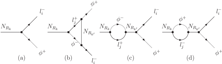
Figure 1: Feynman diagrams of the heavy Majorana neutrino decay: (a) Tree level diagram. One loop diagrams: (b) vertex type and (c) (d) self-energy type diagrams.

Firstly, we calculate the source term $C_{n_{k}}$ in (38). The decays and the inverse decays of the heavy Majorana neutrinos contribute to the source term. The processes involved in the calculation are listed in Table 1. Using the Lagrangian (2), the definitions in Appendix A, and the phase space densities in (39) and (40), we calculate the Feynman diagrams shown in Fig. 1(a) and obtain,

$$C_{n_{k}}^{D} = -\sum\limits_{i}\gamma_{D}^{ki}\left(\frac{n_{k}}{n_{k}^{eq}}-\cosh\frac{\mu_{\phi^{+}}+\mu_{l^{-}_{iL}}}{T}\right),$$ (43)

where $\gamma^{ki}_{D}$ is related to the partial decay width $\Gamma_{ki}(N_{R_{k}}\to l_{i}^{-}\phi^{+})$,

$$\gamma^{ki}_{D}=4n_{k}^{eq}\Gamma_{ki}\frac{K_{1}(z\sqrt{a_{k}})}{K_{2}(z\sqrt{a_{k}})},\ \ \Gamma_{ki}=\frac{1}{32{\pi}}\left|(y_{\nu})_{ik}\right|^{2}M_{k}.$$ (44)

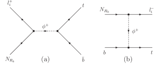
Figure 2: Processes contributing to both the heavy Majorana neutrino densities and lepton number asymmetries with Higgs exchanges via (a) s channel and (b) t channel.

Table 2: The processes with Higgs exchange contributing to the lepton family number densities and heavy Majorana neutrino number densities.

Number change	Processes via t channel		Processes via s channel
${\Delta}L=1,~{}{\Delta}N=1$	$N_{R_{k}}\overline{t}_{R}~{}{\leftrightarrow}~{}l_{i}^{-}\overline{b}_{L}$		$N_{R_{k}}l_{i}^{+}~{}{\leftrightarrow}~{}\overline{b}_{L}t_{R}$
	$N_{R_{k}}b_{L}~{}{\leftrightarrow}~{}l_{i}^{-}t_{R}$		$b_{L}\overline{t}_{R}~{}{\leftrightarrow}~{}N_{R_{k}}l_{i}^{-}$
	$l_{i}^{+}b_{L}~{}{\leftrightarrow}~{}N_{R_{k}}t_{R}$		$t_{L}\overline{t}_{R}~{}{\leftrightarrow}~{}N_{R_{k}}{\nu}_{i}$
	$l_{i}^{+}\overline{t}_{R}~{}{\leftrightarrow}~{}N_{R_{k}}\overline{b}_{L}$	${\gamma}_{{\phi},t}^{ki}$	$N_{R_{k}}\overline{\nu}_{i}~{}{\leftrightarrow}~{}\overline{t}_{L}t_{R}$	${\gamma}_{{\phi},s}^{ki}$
	$N_{R_{k}}t_{L}~{}{\leftrightarrow}~{}t_{R}{\nu}_{i}$
	$\overline{t}_{R}\overline{\nu}_{i}~{}{\leftrightarrow}~{}N_{R_{k}}\overline{t}_{L}$
	$N_{R_{k}}\overline{t}_{R}~{}{\leftrightarrow}~{}\overline{t}_{L}{\nu}_{i}$
	$t_{L}\overline{\nu}_{i}~{}{\leftrightarrow}~{}N_{R_{k}}t_{R}$
source term	$C_{nk}^{(1)R},~{}C_{l_{i}}^{(1)R}$		$C_{nk}^{(2)R},~{}C_{l_{i}}^{(2)R}$

Since the Yukawa coupling of top quark is much larger than those of the other SM particles, the heavy Majorana neutrino creation and annihilation processes in Fig. 2 give important contributions to the heavy Majorana neutrino number densities. [6] The processes are listed in Table 2. Their contributions to the source term $C_{n_{k}}$ are given by,

$$C_{n_{k}}^{R} = C_{n_{k}}^{(1)R}+C_{n_{k}}^{(2)R},$$ (45)

where $C_{n_{k}}^{(1)R}$ and $C_{n_{k}}^{(2)R}$ are,

$$C_{n_{k}}^{(1)R} = -\sum\limits_{i}\gamma^{ki}_{\phi,t}\left[\frac{n_{k}}{n_{k}^{eq}}\left(\cosh\frac{\mu_{t_{L}}}{T}+\cosh\frac{\mu_{t_{R}}}{T}\right)\right.$$ (46)

$$\left.-\cosh\frac{\mu_{l^{-}_{iL}}+\mu_{t_{L}}}{T}-\cosh\frac{\mu_{l^{-}_{iL}}-\mu_{t_{R}}}{T}\right],$$

$$C_{n_{k}}^{(2)R} = -\sum\limits_{i}\gamma^{ki}_{\phi,s}\left[\frac{n_{k}}{n_{k}^{eq}}-\cosh\frac{\mu_{\phi^{+}}+\mu_{l_{iL}^{-}}}{T}\right].$$ (47)

The reaction rates $\gamma_{\phi,s}^{ki}$ and $\gamma^{ki}_{\phi,t}$ are related to the reduced cross sections $\hat{\sigma}^{ki}_{\phi,s}$ and $\hat{\sigma}^{ki}_{\phi,t}$. Their explicit form are given in (122) and (123). The corresponding processes are shown in Fig. 2(a) and Fig. 2(b), respectively.

Next let us study the source terms for lepton family numbers, $C_{l_{i}}$ in (38). The decays and the inverse decays contribution to $C_{l_{i}}^{D}$ is given by,

$$C_{l_{i}}^{D} = \sum\limits_{k}\gamma_{D}^{ki}\left[\varepsilon_{i}^{k}\left(\frac{n_{k}}{n_{k}^{eq}}+\cosh\frac{\mu_{\phi^{+}}+\mu_{l^{-}_{iL}}}{T}\right)+\sinh\frac{\mu_{\phi^{-}}+\mu_{l^{+}_{iL}}}{T}\right],$$ (48)

where the lepton family CP asymmetry $\varepsilon_{i}^{k}$ is defined as,

$$\varepsilon_{i}^{k}=\frac{\Gamma(N_{R_{k}}\to l^{-}_{i}\phi^{+})-\Gamma(N_{R_{k}}\to l^{+}_{i}\phi^{-})}{\Gamma(N_{R_{k}}\to l^{-}_{i}\phi^{+})+\Gamma(N_{R_{k}}\to l^{+}_{i}\phi^{-})}.$$ (49)

The CP asymmetries are generated by the interference of the tree diagram and one-loop diagrams shown in Fig. 1,

$$\varepsilon_{i}^{k} = \frac{1}{8\pi}\sum\limits_{k^{\prime}\neq k}\left[I(x_{k^{\prime}k})\frac{{\rm Im}[(y_{\nu}^{\dagger}y_{\nu})_{kk^{\prime}}(y_{\nu})^{*}_{ik}(y_{\nu})_{ik^{\prime}}]}{|(y_{\nu})_{ik}|^{2}}\right.$$ (50)

$$\left.+\frac{1}{1-x_{k^{\prime}k}}\frac{{\rm Im}[(y_{\nu}^{\dagger}y_{\nu})_{k^{\prime}k}(y_{\nu})^{*}_{ik}(y_{\nu})_{ik^{\prime}}]}{|(y_{\nu})_{ik}|^{2}}\right],$$

where $x_{k^{\prime}k}=M_{k^{\prime}}^{2}/M^{2}_{k}$ and

$$I(x) = \sqrt{x}\left[1+\frac{1}{1-x}+(1+x)\ln\frac{x}{1+x}\right]$$ (53)

$$= \left\{\begin{array}[]{ll}-\frac{3}{2}x^{-1/2}&\ \ \ for\ \ x\gg 1,\\ -2x^{3/2}&\ \ \ for\ \ x\ll 1.\end{array}\right.$$

The diagram Fig. 1(d) gives the contributions to the second terms of the lepton family CP asymmetry (50). The diagram does not contribute to the total lepton asymmetry while it does contribute to the lepton family CP asymmetries.

The contributions to the source term $C_{l_{i}}$ from two particle scatterings can be divided into four parts,

$$C_{l_{i}}^{R}=\sum\limits_{\chi=1}^{4}C_{l_{i}}^{(\chi)R}.$$ (54)

The first two terms in (54) are obtained by calculating the diagrams in Fig. 2. They are given as follows,

$$C_{l_{i}}^{(1)R}\left[\mbox{Fig. \ref{fey3}(b)}\right] = \sum\limits_{k}\gamma^{ki}_{\phi,t}\left[\frac{n_{k}}{n_{k}^{eq}}\left(\sinh\frac{\mu_{t_{L}}}{T}-\sinh\frac{\mu_{t_{R}}}{T}\right)\right.$$ (55)

$$\left.+\sinh\frac{\mu_{l^{+}_{iL}}+\mu_{t_{L}}}{T}+\sinh\frac{\mu_{l^{+}_{iL}}-\mu_{t_{R}}}{T}\right],$$

$$C_{l_{i}}^{(2)R}\left[\mbox{Fig. 2(a)}\right] = \sum\limits_{k}\gamma^{ki}_{\phi,s}\left[\frac{n_{k}}{n_{k}^{eq}}\sinh\frac{\mu_{l^{+}_{iL}}}{T}+\sinh\frac{\mu_{t_{L}}-\mu_{t_{R}}}{T}\right].$$ (56)

The processes listed in Table III also contribute to the $C_{l_{i}}^{R}$. They are denoted by $C_{l_{i}}^{(3)R}$ and $C_{l_{i}}^{(4)R}$ and are given by,

Table 3: $|\Delta L|=2$ and $\Delta L=0$ lepton family number changing scattering processes

Number change	Processes via s (u) channel		Process via t (u) channel
$|{\Delta}L=2|,\ {\Delta}N=0$	$~{}~{}l_{i}^{\pm}{\phi}^{\mp}~{}{\leftrightarrow}~{}l_{j}^{\mp}{\phi}^{\pm}$		${\phi}^{0*}{\phi}^{0*}~{}{\leftrightarrow}~{}{\nu}_{i}{\nu}_{j}$
	$\overline{\nu}_{j}{\phi}^{0*}~{}{\leftrightarrow}~{}{\nu}_{i}{\phi}^{0}$	${\gamma}_{N,1}^{ij}$	$l_{i}^{\pm}l_{j}^{\pm}~{}{\leftrightarrow}~{}{\phi}^{\pm}{\phi}^{\pm}$	${\gamma}_{N,2}^{ij}$
	$\overline{\nu}_{i}{\phi}^{0*}~{}{\leftrightarrow}~{}{\nu}_{j}{\phi}^{0}~{}~{}$		${\phi}^{0}{\phi}^{0}~{}{\leftrightarrow}~{}\overline{\nu}_{i}\overline{\nu}_{j}$
	$\overline{\nu}_{i}{\phi}^{0*}~{}{\leftrightarrow}~{}l_{j}^{-}{\phi}^{+}$		$l_{i}^{-}{\nu}_{j}~{}{\leftrightarrow}~{}{\phi}^{-}{\phi}^{0*}$
	$l_{j}^{+}{\phi}^{-}~{}{\leftrightarrow}~{}{\nu}_{i}{\phi}^{0}$	$\gamma_{N,3}^{ij}$	$l_{i}\overline{\nu}_{j}~{}{\leftrightarrow}~{}{\phi}^{+}{\phi}^{0}$	${\gamma}_{N,t1}^{ij}$
	$l_{i}^{+}{\phi}^{-}~{}{\leftrightarrow}~{}{\nu}_{j}{\phi}^{0}$		$l_{j}^{-}{\nu}_{i}~{}{\leftrightarrow}~{}{\phi}^{-}{\phi}^{0*}$
	$\overline{\nu}_{j}{\phi}^{0*}~{}{\leftrightarrow}~{}l_{i}^{-}{\phi}^{+}$		$l_{j}^{+}\overline{\nu}_{i}~{}{\leftrightarrow}~{}{\phi}^{+}{\phi}^{0}$
$\Delta L=0,\ \Delta L_{i}\neq 0$	$l_{i}^{\pm}{\phi}^{\mp}~{}{\leftrightarrow}~{}l_{j}^{\pm}{\phi}^{\mp}$		${\phi}^{+}{\phi}^{-}~{}{\leftrightarrow}~{}l_{i}^{\pm}l_{j}^{\mp}$
	$\overline{\nu}_{j}{\phi}^{0*}~{}{\leftrightarrow}~{}l_{i}^{+}{\phi}^{-}$		${\nu}_{i}\overline{\nu}_{j}~{}{\leftrightarrow}~{}{\phi}^{0}{\phi}^{0*}$
	$\overline{\nu}_{i}{\phi}^{0*}~{}{\leftrightarrow}~{}\overline{\nu}_{j}{\phi}^{0*}$		${\nu}_{j}\overline{\nu}_{i}~{}{\leftrightarrow}~{}{\phi}^{0}{\phi}^{0*}$
	$\overline{\nu}_{j}{\phi}^{0}~{}{\leftrightarrow}~{}l_{i}^{-}{\phi}^{+}$	${\gamma}_{N,s}^{ij}$	$\nu_{i}l_{j}^{+}~{}{\leftrightarrow}~{}\phi^{+}\phi^{0*}$	${\gamma}_{N,t2}^{ij}$
	$\overline{\nu}_{i}{\phi}^{0*}~{}{\leftrightarrow}~{}l_{j}^{-}{\phi}^{+}$		$\overline{\nu_{i}}l_{j}^{-}~{}{\leftrightarrow}~{}\phi^{0}\phi^{-}$
	${\nu}_{j}{\phi}^{0}~{}{\leftrightarrow}~{}{\nu}_{i}{\phi}^{0}$		$\overline{\nu_{j}}l_{i}^{-}~{}{\leftrightarrow}~{}\phi^{0}\phi^{-}$
	$l_{j}^{-}{\phi}^{+}~{}{\leftrightarrow}~{}{\nu}_{i}{\phi}^{0}$		$\nu_{j}l_{i}^{+}{\leftrightarrow}~{}\phi^{+}\phi^{0*}$
source term	$C_{l_{i}}^{(3)R}$		$C_{l_{i}}^{(4)R}$

$$C_{l_{i}}^{(3)R} = -\sum\limits_{j,k}\frac{|(y_{\nu})_{jk}|^{2}}{(y_{\nu}^{\dagger}y_{\nu})_{kk}}\gamma_{D}^{ki}\left[\varepsilon_{i}^{k}\left(\cosh\frac{\mu_{\phi^{-}}+\mu_{l_{iL}^{+}}}{T}+\cosh\frac{\mu_{\phi^{-}}+\mu_{l_{jL}^{+}}}{T}\right)\right.$$ (57)

$$\left.+\sinh\frac{\mu_{\phi^{-}}+\mu_{l_{iL}^{+}}}{T}\right]+\sum\limits_{j}(\gamma^{ij}_{N,1}+\gamma^{ij}_{N,3})\left(\sinh\frac{\mu_{\phi^{-}}+\mu_{l_{iL}^{+}}}{T}+\sinh\frac{\mu_{\phi^{-}}+\mu_{l_{jL}^{+}}}{T}\right)$$

$$+2\sum\limits_{j}\gamma^{ij}_{N,s}\left(\sinh\frac{\mu_{\phi^{-}}+\mu_{l_{iL}^{+}}}{T}-\sinh\frac{\mu_{\phi^{-}}+\mu_{l_{jL}^{+}}}{T}\right),$$

$$C_{l_{i}}^{(4)R} = \sum\limits_{j}\left[\left(\frac{1}{2}\gamma^{ij}_{N,2}+\gamma^{ij}_{N,t1}\right)\left(\sinh\frac{2\mu_{\phi^{-}}}{T}+\sinh\frac{\mu_{l^{+}_{iL}}+\mu_{l_{jL}^{+}}}{T}\right)\right.$$ (58)

$$\left.+2\gamma^{ij}_{N,t2}\sinh\frac{\mu_{l_{iL}^{+}}-\mu_{l_{jL}^{+}}}{T}\right].$$

The processes in Table III are classified into the total lepton number changing scatterings ($|\Delta L|=2$) and the total lepton number conserving scatterings ($\Delta L=0$).

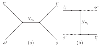
Figure 3: The lepton family number violating scatterings with $N_{R_{k}}$ exchanges via (a) s channel and (b) u channel.

In the former, the lepton family number $L_{i}$ changes by one unit or by two units. The latter corresponds to $|\Delta L_{i}|=1$. The total lepton number conserving and the lepton family number violating processes must be taken into account when we study each lepton family number evolution. In Fig. 3, the typical Feynman diagrams which correspond to $\Delta L=0$ $\Delta L_{i}=-1$ are shown. Their reaction rates are included in $\gamma_{N,s}$ and $\gamma_{N,t2}$ of (57) and (58). Finally we also note that in (57), the term ${\varepsilon}_{i}^{k}$ comes from the on-shell contribution of s-channel heavy Majorana particle exchanged diagrams.

3.2 Sphaleron and chemical potential relations

In the previous subsection, we write the source terms with the reaction rates $\gamma$ and the chemical potentials $\mu$. In this subsection, we derive the relation between the lepton family asymmetries $Y_{Li}$ and chemical potentials by considering the various equilibrium conditions. We adapt the method developed by Harvey and Turner.  [13] [14]

At first, let us consider the effective action of sphaleron for all left-handed fermions,

$${\cal O}_{B+L}=\prod_{i}(Q_{i}Q_{i}Q_{i}L_{i}),$$ (59)

where $Q_{i},L_{i}$ are quark and lepton doublets respectively. The sphaleron transition rate at high temperature, in the symmetric phase, is estimated to be [12]

$${\Gamma}_{\rm sph}~{}{\sim}~{}2{\times}10^{2}{\alpha}_{W}^{5}T,$$ (60)

where ${\alpha}_{W}$ is weak coupling constant at Grand Unified scale and is taken to be $\frac{1}{40}$. From the thermal equilibrium condition, i.e., ${\Gamma}_{\rm sph}>H$ , we obtain the upper bound of the temperature $T_{\rm sph}=1.4{\times}10^{12}~{}{\rm[GeV]}$. Above the temperature, sphaleron process is not active. At low energy, below $T_{\rm EW}\simeq 10^{2}~{}[\rm{GeV}]$, the sphaleron process is frozen out again, then the active temperature range of sphaleron is,

$$T_{\rm EW}\leq T\leq T_{\rm sph}.$$ (61)

In the temperature range (61), the sphaleron equilibrium condition leads to the chemical potential relation,

$$\sum_{i=1}^{N_{f}}\left({\mu}_{u_{iL}}+2{\mu}_{d_{iL}}+{\mu}_{i{\nu}}\right)=0.$$ (62)

where $N_{f}=3$. We assume that gauge and Yukawa interactions are in equilibrium. From charged current interaction processes, we obtain the following chemical potential relations,

$${\mu}_{W^{-}}={\mu}_{d_{iL}}-{\mu}_{u_{iL}}={\mu}_{l^{-}_{iL}}-{\mu}_{{\nu}_{iL}}={\mu}_{{\phi}^{-}}+{\mu}_{{\phi}^{0}},$$ (63)

where $i~{}(i=1,2,3)$ denote indices for the generations. By taking the weak basis that the Yukawa term for up type quarks is flavor diagonal and that for down type quarks has flavor off-diagonal elements, we obtain the chemical potential relations from the equilibrium condition of the Yukawa interactions,

$${\mu}_{{\phi}^{0}}={\mu}_{u_{iR}}-{\mu}_{u_{iL}}={\mu}_{d_{iL}}-{\mu}_{d_{jR}}={\mu}_{l^{-}_{iL}}-{\mu}_{l^{-}_{iR}},$$ (64)

where we note that the chemical potentials for the left-handed down quarks ($d_{iL}$) and those of the right-handed down quarks ($d_{jR}$) satisfy the flavor mixed relations. Therefore the chemical potentials for the right-handed down quarks and the left-handed down quarks are flavor independent. Both of them can be written by a single chemical potential as,

$$\mu_{d_{iR}}=\mu_{d_{R}},\quad\mu_{d_{iL}}=\mu_{d_{L}}.$$ (65)

Using (63),(64) and (65), we can also show that the chemical potentials for up type quarks are flavor independent,

$$\mu_{u_{iR}}=\mu_{u_{R}},\quad\mu_{u_{iL}}=\mu_{u_{L}}.$$ (66)

Next, we can relate the chemical potentials of SU(2) doublets. This follows from the chemical potential for $W$ boson vanishes in the symmetric phase. [13]. From (63), the up and down components of SU(2) doublets have the same chemical potential. Note that the chemical potentials for leptons can be flavor dependent.

$${\mu}_{l^{-}_{iL}}={\mu}_{{\nu}_{iL}}={\mu}_{l^{-}_{iR}}+\mu_{\phi^{0}}.$$ (67)

We also take into account of the charge neutrality condition. The condition can be written as,

$$Q = \frac{T^{2}}{3}\left[\sum_{i=1}^{N_{f}}{\mu}_{u_{iL}}-{\mu}-\left(2N_{f}+N_{H}+2\right){\mu}_{W^{-}}+(2N_{f}+N_{H}){\mu}_{{\phi}^{0}}\right]=0,$$

where ${\mu}{\equiv}\sum\limits_{i}{\mu}_{{\nu}_{iL}}$ and $N_{H}$ is the number of Higgs doublet and is taken to be $1$. With (62),(65),(66), (LABEL:charge) and $\mu_{W}=0$, we obtain the following relations,

$$9\mu_{\mu_{L}}+\mu=0$$

$$3\mu_{\mu_{L}}=\mu-7\mu_{\phi^{0}}.$$ (69)

Then the chemical potentials for quarks and charged leptons can be written by the single chemical potential of $\mu=\sum\limits_{i}{\mu}_{{\nu}_{iL}}$ of neutrinos as follows:

$$\begin{array}[]{lll}\mu_{u_{L}}=\mu_{d_{L}}=-\frac{1}{9}\mu,&\mu_{u_{R}}=\frac{5}{63}\mu,&\mu_{d_{R}}=-\frac{19}{63}\mu,\\ \mu_{\phi^{0}}=-\mu_{\phi^{-}}=\frac{4}{21}\mu,&\sum\limits_{i}\mu_{l^{-}_{iL}}=\mu,\\ \sum\limits_{i}\mu_{l^{-}_{iR}}=\frac{3}{7}\mu.\\ \end{array}$$ (73)

We can also write the baryon number density and lepton number densities with the chemical potentials as,

$$n_{Li} = \frac{T^{2}}{6}(\mu_{{\nu}_{iL}}+{\mu}_{l_{iL}^{-}}+{\mu}_{l_{iR}^{-}})=\frac{T^{2}}{2}\left({\mu}_{l_{iL}^{-}}-\frac{4}{63}{\mu}\right),$$

$$n_{L} = \sum_{i=1}^{N_{f}}n_{Li}=\frac{T^{2}}{2}\left({\mu}-\frac{4}{21}{\mu}\right)=\frac{17}{42}T^{2}{\mu},$$ (74)

$$n_{B} = \frac{T^{2}}{6}\sum_{i=1}^{N_{f}}({\mu}_{u_{iL}}+{\mu}_{u_{iR}}+{\mu}_{d_{iL}}+{\mu}_{d_{iR}})=N_{f}\left(\frac{2}{3}T^{2}{\mu}_{u_{L}}\right)=-\frac{2}{9}T^{2}{\mu}.$$

By using the equations above, we finally obtain the relations between the chemical potentials for the lepton doublets ($\mu_{l^{-}_{iL}}$) and lepton family asymmetries,

$$Y_{L_{i}} = \frac{n_{L_{i}}}{s}=\frac{1}{2}\left(\frac{{\mu}_{l_{iL}^{-}}}{T}\right)\frac{T^{3}}{s}-\frac{4}{51}Y_{L},$$

$$Y_{L} = \frac{n_{L}}{s}=\frac{17}{42}\left(\frac{{\mu}}{T}\right)\frac{T^{3}}{s},$$ (75)

where $s$ is entropy density given by $s=\frac{2\pi^{2}}{45}g_{*}\left(\frac{M_{1}}{z}\right)^{3}.$ What is important particularly from the flavor-dependent point of view is that family asymmetry $Y_{L_{i}}$ take a different value on the each generation. The conversion rate from lepton asymmetry to baryon asymmetry is given by the well known formulae [13],

$$Y_{B}=-\frac{28}{51}Y_{L}.$$ (76)

We will use the relations (73) and (75) to express all the chemical potentials in terms of the lepton family asymmetries in the next subsection.

3.3 Boltzmann Equations

Now we can write the Boltzmann equations in a tractable form. Using the definition in (3.2),$Y_{N_{k}}=\frac{n_{k}}{s}$ and $Y_{L}^{eq}=\frac{T^{3}}{s}$, the Boltzmann equations (38) can be rewritten as,

$$\frac{dY_{N_{k}}}{dz} = -\frac{z}{sH(1)}\left(\frac{Y_{N_{k}}}{Y_{N_{k}}^{eq}}-1\right)\sum_{i}\left[{\gamma}_{D}^{ki}+{\gamma}_{{\phi},s}^{ki}+2{\gamma}_{{\phi},t}^{ki}\right],$$

$$\frac{dY_{L_{i}}}{dz} = -\frac{z}{sH(1)}\left\{-\sum_{k}\left(\frac{Y_{N_{k}}}{Y_{N_{k}}^{eq}}-1\right){\varepsilon}_{i}^{k}{\gamma}_{D}^{ki}\right.$$ (77)

$$\left.+\sum_{j}\frac{Y_{L_{j}}}{Y_{L}^{eq}}\left[A_{ij}+\sum_{k}\frac{Y_{N_{k}}}{Y_{N_{k}^{eq}}}A_{ij}^{k}\right]\right\},$$

where the time $t$ derivative in (38) is replaced by derivative on $z$ using the relation in the radiation-dominated epoch,

$$t = \frac{1}{2H(1)}z^{2},$$

$$H(1) = \sqrt{\frac{4\pi^{3}g_{*}}{45}}\frac{M_{1}^{2}}{m_{P}}.$$ (78)

In the source terms $C_{l_{i}}^{D,R}$, $C_{n_{k}}^{D,R}$ derived in subsection 3.1, we adapt the chemical potential relations in (73) and (75), and the approximation of $\sinh\frac{\mu_{X}}{T}\simeq\frac{\mu_{X}}{T}$,   $\cosh\frac{\mu_{X}}{T}\simeq 1$. Then $A_{ij}$ and $\ A_{ij}^{k}$ are given as follows,

$$A_{ij} = 16\sum_{j^{\prime}}^{3}\left[\left(\frac{1}{8}({\delta}_{ij}+{\delta}_{jj^{\prime}})+\frac{4}{51}\right)\left({\gamma}_{N,1}^{ij^{\prime}}+{\gamma}_{N,3}^{ij^{\prime}}\right)+\left(\frac{2}{51}+\frac{1}{16}({\delta}_{ij}+{\delta}_{jj^{\prime}})\right){\gamma}_{N,2}^{ij^{\prime}}\right.$$ (79)

$$\left.+\left(\frac{1}{8}({\delta}_{ij}+\delta_{jj^{\prime}})+\frac{4}{51}\right){\gamma}_{N,t1}^{ij^{\prime}}+\frac{1}{4}({\delta}_{ij}-\delta_{jj^{\prime}})\left({\gamma}_{N,t2}^{ij^{\prime}}+{\gamma}_{N,s}^{ij^{\prime}}\right)\right]$$

$$+8\sum_{k}\left[\left(\frac{1}{2}{\delta}_{ij}+\frac{5}{51}\right){\gamma}_{{\phi},t}^{ki}+\frac{1}{17}{\gamma}_{{\phi},s}^{ki}\right],$$

$$A_{ij}^{k} = 2\left[\frac{4}{17}{\gamma}_{{\phi},t}^{ki}+\left({\delta}_{ij}+\frac{4}{51}\right){\gamma}_{{\phi},s}^{ki}\right].$$ (80)

4 Numerical results

In this section, we present the numerical results for the lepton family number asymmetries based on the minimal seesaw model described in Sec. 2. As we showed in the previous section, the Yukawa coupling $y_{\nu}=\frac{\sqrt{2}m_{D}}{v}$, and the heavy Majorana masses $M_{1}$,$M_{2}$ are needed for the numerical analysis of Boltzmann equation. We parameterize $m_{D}$ in the bi-unitary form, i.e., $m_{D}=U_{L}mV_{R}$ and write the parameters in $m$ and $V_{R}$ with $M_{1},R=\frac{M_{1}}{M_{2}},x_{1},x_{2},n_{2}$ and $n_{3}$.

Next we show how the angles in $U_{L}$ are constrained by discussing the presently available neutrino oscillation experimental measurements. The SK Collaboration showed that the $\nu_{\mu}$ created in the atmosphere oscillates into $\nu_{\tau}$ with almost maximal mixing [15], $\sin^{2}2\theta_{atm}\sim 1$ and the neutrino mass squared difference $\Delta m^{2}_{atm}=(2\sim 4)\times 10^{-3}~{}{\rm[eV^{2}]}$. The second mass-squared difference and mixing angle are constrained by solar neutrino experiments. The SNO collaboration reported that the $\nu_{e}$’s from the sun oscillate into the other active neutrinos [16]. The SK and the SNO collaboration [16] suggested that the MSW large-mixing-angle (LMA) solution is the most favorable solution to the solar-neutrino deficit problem, for which $\sin^{2}2\theta_{sol}=0.7\sim 0.9$ and the combined analysis of the KamLAND [17] and all the solar neutrino data gives $\Delta m^{2}_{sol}=(3\sim 15)\times 10^{-5}~{}{\rm[eV^{2}]}$. For the third mixing angle, only the upper bound is obtained from the reactor neutrino experiments. CHOOZ [18] found $\sin^{2}2\theta_{rea}<0.1$ for $\Delta m^{2}_{atm}\sim 3\times 10^{-3}~{}{\rm[eV^{2}]}$. The current neutrino experimental data indicates clearly that there is a hierarchy of neutrino mass-splitting. If the small mixing angles $\theta_{L13}$ and $\theta$ are taken, the light neutrinos mixing matrix $U_{MNS}$ defined in (29), can be simplified,

$$U_{MNS}\simeq\left(\begin{array}[]{ccc}\cos\theta_{L12}&\sin\theta_{L12}&\begin{array}[]{c}\sin\theta_{L13}e^{-i\delta_{L}}+\\ \sin\theta_{L12}\sin\theta e^{-i\phi^{\prime}}\end{array}\\ -\sin\theta_{L12}\cos\theta_{L23}&\cos\theta_{L12}\cos\theta_{L23}&\sin\theta_{L23}\\ \sin\theta_{L12}\sin\theta_{L23}&-\cos\theta_{L12}\sin\theta_{L23}&\cos\theta_{L23}\end{array}\right)P(\alpha^{\prime}),$$ (86)

(87)

where $\phi^{\prime}=\phi+\gamma_{L}$, $\alpha^{\prime}=\alpha-\gamma_{L}/2$ and $P(\alpha^{\prime})=diag.(1,e^{i\alpha^{\prime}},e^{-i\alpha^{\prime}})$. A very similar form to the low energy MNS mixing matrix is obtained. In this case, the angles in matrix $U_{L}$ defined in (17) can be related directly to the corresponding neutrino mixing angles and can be determined by neutrino experiments. In this work, we take the natural hierarchical scenario and set the following neutrino masses in (37) for the corresponding measured neutrino mass differences,

$$n_{2}=\sqrt{\Delta m^{2}_{sol}}=7\times 10^{-3}~{}\mbox{[eV]},\ \ n_{3}=\sqrt{\Delta m^{2}_{atm}}=5\times 10^{-2}~{}\mbox{[eV]}.$$ (88)

For the angles in $U_{L}$, we can take,

$$\theta_{L12}=\theta_{sol}=\frac{\pi}{6},\ \ \theta_{L23}=\theta_{atm}=\frac{\pi}{4}.$$ (89)

The parameters $x_{1,2}$ defined in (27) are constrained by the conditions [11],

$$|x_{1}-x_{2}|\leq n_{3}-n_{2},\ \ n_{3}+n_{2}\leq x_{1}+x_{2}.$$ (90)

The primordial lepton number must be created when the sphaleron process is in equilibrium so that the conversion from the lepton numbers to the baryon number occurs effectively. In our numerical calculation, we fix the mass for the lightest heavy Majorana neutrino $M_{1}$ as $2\times 10^{11}$ [GeV], below $T_{\rm sph}\simeq 10^{12}$ [GeV] and we take the ratio $R=\frac{M_{1}}{M_{2}}$ to be $0.1$. Finally, we consider the constraints from measurements of the cosmological baryon to photon ratio $\eta=n_{B}/n_{\gamma}$[1, 2]. Recall that temperature below $T_{\rm EW}$, sphaleron process is not active and thus, the total baryon number $B$ is conserved.

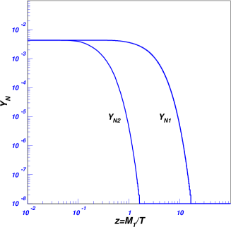
Figure 4: The evolution of the heavy Majorana Neutrino densities.

If the universe expands adiabatically, the total entropy $S$ is also conserved. Then $Y_{B}$ is also conserved as,

$$Y_{B}(T_{\rm EW})=Y_{B}(T_{0}=3{\rm K})\simeq\frac{1}{7}\eta.$$

(91)

Substituting (91) into (76) and combining the measurements in (1), we infer the bounds on the primordial lepton asymmetry $Y_{L}=n_{L}/s$ that we have to generate,

$$Y_{L}(T_{\rm EW})=-\frac{51}{196}\eta$$ (92)

$$= -(1.15-2.13)\times 10^{-10},$$

at 90% C.L.
We take the following values for the other parameters;

$$\sin\theta_{L13}e^{-i\delta_{L}}=0,\quad(x_{1},x_{2})=(0.0523,0.0100)~{}{\mbox{\rm{[eV]}}}.$$ (93)

Concerning Higgs mass $m_{H}$, we change it from $150$(GeV) to $800$(GeV) and the results are not sensitive to the choice. So we show the figures for $m_{H}=800~{}{\mbox{\rm{[GeV]}}}.$ With them, only the CP violating phase $\gamma_{L}$ is the parameter which remains to be fixed.

To solve the Boltzmann equation, we start at $T\gg M_{1}$ ($z=10^{-2}$) with the initial conditions,

$$Y_{N_{k}}=Y_{N_{k}}^{eq},\ \ Y_{L_{i}}=0.$$ (94)

The typical results are displayed in Fig. 4 to Fig. 8. Fig. 4 shows the dependence of the heavy Majorana neutrino density to entropy density ratios $Y_{N}$ on temperature. One can see clearly that for high temperature region $z\leq 0.1$, $Y_{N_{1}}$ is nearly equal to $Y_{N_{2}}$. However, as $z$ becomes larger, the asymmetry from the heavier right-handed neutrino decays drops quickly, thus, the lighter one gives dominate contribution.

We plot the evolution of the lepton family asymmetries in Fig. 5, Fig. 6 and Fig. 7. By investigating the family structure of these figures, we observe the following features.

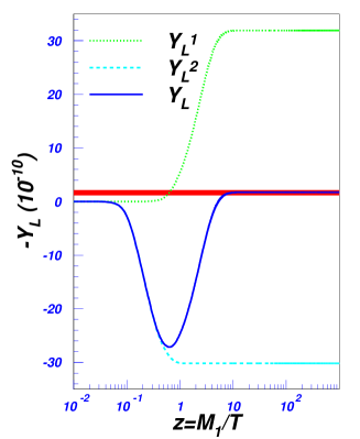
Figure 5: The lepton asymmetry $Y_{L}^{1}\ (Y_{L}^{2})$ from $N_{R_{1}}$ ($N_{R_{2}}$) decay. The total lepton asymmetry is denoted by $Y_{L}$. $\gamma_{L}=0$. The shaded part shows the bounds on $Y_{L}$ in (92) via experimental measurements [1, 2] at 90% C.L.

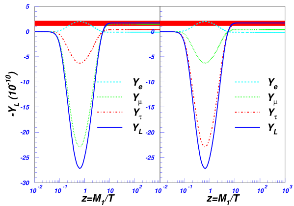
Figure 6: The evolution of the lepton asymmetry and lepton family asymmetries with the CP violating phase ${\gamma}_{L}=0$ (left) and $\gamma_{L}=\pi$ (right).

(1) The total lepton asymmetry $Y_{L}$ increases with larger $z$ and reach its maximum at $z\sim 0.6$. The behavior of $Y_{L}$ in small $z$ region can be understood as follows. Since ${\rm Im}[(y_{\nu}^{\dagger}y_{\nu})^{2}]_{12}=-{\rm Im}[(y_{\nu}^{\dagger}y_{\nu})^{2}]_{21}$, the term $\sum\limits_{i}\left(\frac{Y_{N_{k}}}{Y_{N_{k}}^{eq}}-1\right){\varepsilon}_{i}^{k}{\gamma}_{D}^{ki}$ in (77) is positive for $k=2$ while negative for $k=1$. In addition, for $R\ll 1$, from Eqs. (50), (53) and (44), one can obtain that the order of $\sum\limits_{i}\varepsilon_{i}^{k}\gamma_{D}^{ki}$ is the same for $k=1$ and $k=2$. However, around $z\simeq 0.1$, the deviation from equilibrium distribution is larger for the heavier Majorana neutrion $N_{R_{2}}$. Thus, the magnitude of the positive one is much larger than the negative one. Then, $Y_{L}$ increases in the small $z$ region. This feature is in contrast to the previous work [11] where only contribution from the lighter right-handed neutrino $N_{R_{1}}$ are taken into account. As $z$ becomes larger, the positive contribution to $Y_{L}$ from the heavier Majorana neutrinos decreases and the contribution from the lightest heavy Majorana neutrinos decay becomes dominant. We can see that the sign of $Y_{L}$ changes at the intermediate regions ($1<z<10$). Then the lepton asymmetry from the the heavier Majorana neutrino ($N_{R_{2}}$) is compensated by the one from the lightest heavy Majorana neutrino ($N_{R_{1}}$). This feature can be seen clearly by showing the contribution to lepton asymmetry from $N_{R_{1}}$ and $N_{R_{2}}$ decays separately, as desplayed in Fig. 5. $Y_{L}$ will further decrease and it tends to be a constant asymptotically at low temperature. It is important to include the contributions from both heavy Majorana neutrinos for the lepton asymmetry and its evolution.

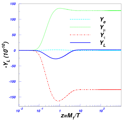
Figure 7: The evolution of the lepton asymmetry and lepton family asymmetries with the CP violating phase $\gamma_{L}=\frac{\pi}{2}$.

(2) In Fig. 6, we have shown the lepton family asymmetries for the two different choices of CP violating phase $\gamma_{L}$. The figure on the left corresponds to $\gamma_{L}=0$ and that on the right corresponds to $\gamma_{L}=\pi$. Despite of similarity in their shapes, the dominant contribution to $Y_{L}$ comes from $Y_{\mu}$ for $\gamma_{L}=0$, whereas, $Y_{\tau}$ in case of $\gamma_{L}=\pi$. The results indicate the lepton family asymmetries $Y_{L_{i}}$ are sensitive to the CP violating phase $\gamma_{L}$. To understand about the feature (2), let us focus attention again on term ${\varepsilon}_{i}^{k}{\gamma}_{D}^{ki}$ in (77) which is propotental to $Im[(y_{\nu}^{\dagger}y_{\nu})_{12}(y_{\nu})^{*}_{i1}(y_{\nu})_{i2}]$. Since the matrix $y_{\nu}^{\dagger}y_{\nu}$ is not related to the matrix $U_{L}$, and $\gamma_{L}$ just appears in matrix $U_{L}$ (17), the $\gamma_{L}$-dependent terms in ${\varepsilon}_{i}^{k}{\gamma}_{D}^{ki}$ only come from the quantity $(y_{\nu})^{*}_{i1}(y_{\nu})_{i2}$ in (50). Using (17) and (25), we otbain

$$(y_{\nu})^{*}_{i1}(y_{\nu})_{i2} = \frac{2}{v^{2}}e^{i\gamma_{R}}\left\{(m_{2}^{2}-m_{3}^{2})\sin\theta_{R}\cos\theta_{R}\left(|(U_{L})_{i2}|^{2}-|(U_{L})_{i3}|^{2}\right)\right.$$ (95)

$$\left.+m_{2}m_{3}\left[\cos^{2}\theta_{R}(U_{L})^{*}_{i2}(U_{L})_{i3}-\sin^{2}\theta_{R}(U_{L})_{i2}(U_{L})^{*}_{i3}\right]\right\}.$$

Note only the second term of (95) is relevant to CP phase $\gamma_{L}$, and is proportional to $(U^{*}_{L})_{i2}(U_{L})_{i3}$ given by

$$(U^{*}_{L})_{12}(U_{L})_{13} = \frac{1}{2}\sin 2\theta_{L13}\sin\theta_{L12}e^{i({\gamma}_{L}-{\delta}_{L})}\simeq 0,$$

$$(U^{*}_{L})_{22}(U_{L})_{23} = \frac{1}{2}\left(-\sin 2\theta_{L13}\sin\theta_{L12}\sin^{2}\theta_{L23}e^{-i{\delta}_{L}}\right.$$

$$\left.+\cos\theta_{L12}\cos\theta_{L13}\sin 2\theta_{L23}\right)e^{i{\gamma}_{L}}\simeq\frac{\sqrt{6}}{8}e^{i{\gamma}_{L}},$$

$$(U^{*}_{L})_{32}(U_{L})_{33} = \frac{1}{2}\left(-\sin 2\theta_{L13}\sin\theta_{L12}\cos^{2}\theta_{L23}e^{-i{\delta}_{L}}\right.$$ (96)

$$\left.-\cos\theta_{L12}\cos\theta_{L13}\sin 2\theta_{L23}\right)e^{i{\gamma}_{L}}\simeq-\frac{\sqrt{6}}{8}e^{i{\gamma}_{L}}.$$

From (95) and (96) that in cases of $\gamma_{L}=0,\pi$, the $\gamma_{L}$-dependent terms of ${\varepsilon}_{i}^{k}{\gamma}_{D}^{ki}$ have opposite sign, leading to that $Y_{\mu}$ is dominant in the total lepton asymmetry in case of $\gamma_{L}=0$, while $Y_{\tau}$ is dominant in case of $\gamma_{L}=\pi$. In Fig.  7, we have shown the evolution of the lepton family asymmetries for another choice, $\gamma_{L}=\frac{\pi}{2}$. In this case, $|Y_{\mu}|$ and $|Y_{\tau}|$ are much larger than $Y_{L}$. In contrast to the total lepton asymmetry, the lepton family asymmetry, for example, $Y_{\mu}$ from $N_{R_{2}}$ decay is dominant and can not be upset by the contribution from $N_{R_{1}}$ decay.

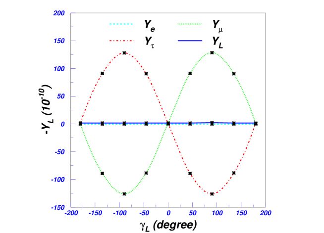
Figure 8: The lepton family asymmetries as a function of the CP phase $\gamma_{L}$. The data points denoted with star are extrapolated.

The understanding is illustrated in Fig. 8. We show the lepton asymmetries at the low energy and study the dependence of the asymptotic ($z\gg 1$) values on the CP violating phase $\gamma_{L}$. In contrast to case of $Y_{\mu}$ and $Y_{\tau}$, $Y_{e}$ and the total lepton asymmetry $Y_{L}$ is insensitive to the value of CP phase $\gamma_{L}$ and is nearly constant. In addition, we find from this figure that for the inputs we chose, the size of the lepton family asymmetries $Y_{\mu}$ and $Y_{\tau}$ can be of order $10^{-8}$ and cancel each other mostly, leaving the total lepton asymmetry of order $10^{-10}$ which is consistent with the experimental observations [1, 2].

5 Conclusions

In this work we have presented a detailed calculations for primordial lepton family asymmetries in seesaw model by taking into account the effect of chemical potentials for all SM particles. The $minimal$ CP violating seesaw model is used in obtaining numerical results. The main results of our paper are as follows.
(1) Subject to constraints from neutrino oscillation experiments and observed cosmological baryon to photon ratio, the order of the total lepton asymmetry $Y_{L}$ can be different from that for each generations $Y_{L_{i}}$. There exist scenarios in the minimal seesaw model, both $Y_{\mu}$ and $Y_{\tau}$ are of order $10^{-8}$, whereas $Y_{L}$ is of order $10^{-10}$ due to the cancellation.
(2) The lepton family asymmetries are sensitive to CP violating phase $\gamma_{L}$ in the matrix $U_{L}$. In contrast to this, the dependence of the total lepton asymmetry on $\gamma_{L}$ is quite weak. Note that the total lepton asymmetry is sensitive to the CP violating phase $\gamma_{R}$ in $V_{R}$ [11].
(3) Both of the heavy Majorana neutrinos give important contributions to the primordial lepton family asymmetries. The heavier Majorana neutrino decay can dominate in the lepton family asymmetry.
The new features we found provide useful informations and may be observable in future cosmological experiments. As a future extension of the research, it would be interesting to investigate the correlation between CP violation for the lepton family asymmetries and the low energy CP violation of neutrino oscillations [19, 20, 21, 22, 23].

Appendix A Source terms $C_{l_{i}}$ and $C_{n_{k}}$

In this Appendix, we show the definitions of the source terms $C_{l_{i}}$ and $C_{n_{k}}$. Writing the source term as $C_{l_{i}}=C_{l_{i}}^{D}+C_{l_{i}}^{R}$, $C_{l_{i}}^{D}$ and $C_{l_{i}}^{R}$ stand for contributions from the decays and the inverse decays of the heavy Majorana neutrinos and two-body scatterings, respectively. $C_{l_{i}}^{D}$ is defined as,

$$C_{l_{i}}^{D} = \int d\Pi_{1}d\Pi_{2}d\Pi_{N}(2{\pi})^{4}{\delta}^{4}(p_{1}+p_{2}-p_{N}){\times}$$ (97)

$$\sum\limits_{k,s_{z}}\left\{f_{N}(s_{z})\left[\left|{\cal M}(N_{R_{k}}(s_{z}){\rightarrow}l_{i}^{-}{\phi}^{+})\right|^{2}(1+f_{{\phi}^{+}})(1-f_{l_{i}^{-}})\right.\right.$$

$$+\left.\left.\left|{\cal M}(N_{R_{k}}(s_{z}){\rightarrow}{\nu}_{i}{{\phi}^{0}})\right|^{2}(1+f_{{\phi}^{0}})(1-f_{{\nu}_{i}})\right.\right.$$

$$-\left.\left.\left|{\cal M}(N_{R_{k}}(s_{z}){\rightarrow}l_{i}^{+}{\phi}^{-})\right|^{2}(1+f_{{\phi}^{-}})(1-f_{l_{i}^{+}})\right.\right.$$

$$\left.\left.-\left|{\cal M}(N_{R_{k}}(s_{z}){\rightarrow}\overline{\nu}_{i}{{\phi}^{0}}^{*})\right|^{2}(1+f_{{{\phi}^{0*}}})(1-f_{\overline{\nu}_{i}})\right]\right.$$

$$+\left.(1-f_{N}(s_{z}))\left[f_{{\phi}^{-}}f_{l_{i}^{+}}\left|{\cal M}(l_{i}^{+}{\phi}^{-}{\rightarrow}N_{R_{k}}(s_{z}))\right|^{2}\right.\right.$$

$$\left.\left.+f_{{{\phi}^{0}}^{*}}f_{\overline{\nu}_{i}}\left|{\cal M}(\overline{\nu}_{i}{{\phi}^{0}}^{*}{\rightarrow}N_{R_{k}}(s_{z}))\right|^{2}\right.\right.$$

$$\left.\left.-f_{{{\phi}^{+}}}f_{l^{-}_{i}}\left|{\cal M}(l_{i}^{-}{\phi}^{+}{\rightarrow}N_{R_{k}}(s_{z}))\right|^{2}\right.\right.$$

$$\left.\left.-f_{{\nu}_{i}}f_{{\phi}^{0}}\left|{\cal M}({\nu}_{i}{\phi}^{0}{\rightarrow}N_{R_{k}}(s_{z}))\right|^{2}\right]\right\},$$

where $d\Pi_{i}=\frac{d^{3}p_{i}}{(2{\pi})^{3}2E_{i}}$ and $\left|{\cal M}(a+b+{\cdots}{\rightarrow}i+j+{\cdots})\right|^{2}$ stands for the amplitude squared for the process $a+b+{\cdots}{\rightarrow}i+j+{\cdots}$.

The contributions from two particles scattering processes can be divided into four parts,

$$C_{l_{i}}^{R}=C_{l_{i}}^{(1)R}+C_{l_{i}}^{(2)R}+C_{l_{i}}^{(3)R}+C_{l_{i}}^{(4)R}.$$ (98)

The terms $C_{l_{i}}^{(\chi)R}\ (\chi=1,2,3,4)$ are defined as follows,

$$C_{l_{i}}^{(1)R} = \int d\Pi_{1}d\Pi_{2}d\Pi_{3}d\Pi_{4}(2\pi)^{4}\delta^{4}(p_{1}+p_{2}-p_{3}-p_{4})\times$$ (99)

$$\sum_{k,s_{z},\alpha}\left[f_{N}(s_{z})f_{\bar{t}^{\alpha}_{R}}|{\cal M}(N_{R_{k}}(s_{z})\overline{t}_{R}^{\alpha}{\rightarrow}l_{i}^{-}\overline{b}_{L}^{\alpha})|^{2}(1-f_{l_{i}^{-}})(1-f_{\bar{b}^{\alpha}_{L}})\right.$$

$$\left.+f_{N}(s_{z})f_{b^{\alpha}_{L}}|{\cal M}(N_{R_{k}}(s_{z})b^{\alpha}_{L}{\rightarrow}l_{i}^{-}t^{\alpha}_{R})|^{2}(1-f_{l_{i}^{-}})(1-f_{t^{\alpha}_{R}})\right.$$

$$\left.-f_{N}(s_{z})f_{t^{\alpha}_{R}}|{\cal M}(N_{R_{k}}(s_{z})t_{R}^{\alpha}{\rightarrow}l_{i}^{+}b_{L}^{\alpha})|^{2}(1-f_{l_{i}^{+}})(1-f_{t_{R}^{\alpha}})\right.$$

$$\left.-f_{N}(s_{z})f_{\overline{b}_{L}^{\alpha}}|{\cal M}(N_{R_{k}}(s_{z})\overline{b}_{L}^{\alpha}{\rightarrow}l_{i}^{+}\overline{t}_{R}^{\alpha})|^{2}(1-f_{l_{i}^{+}})(1-f_{t_{R}^{\alpha}})\right.$$

$$\left.+f_{N}(s_{z})f_{\overline{t}^{\alpha}_{R}}|{\cal M}(N_{R_{k}}(s_{z})\overline{t}^{\alpha}_{R}{\rightarrow}{\nu}_{i}\overline{t}^{\alpha}_{L})|^{2}(1-f_{{\nu}_{i}})(1-f_{\overline{t}^{\alpha}_{L}})\right.$$

$$\left.+f_{N}(s_{z})f_{t^{\alpha}_{L}}|{\cal M}(N_{R_{k}}(s_{z}){t}_{L}^{\alpha}{\rightarrow}{\nu}_{i}t^{\alpha}_{R})|^{2}(1-f_{{\nu}_{i}})(1-f_{t_{R}^{\alpha}})\right.$$

$$\left.-f_{N}(s_{z})f_{t_{R}^{\alpha}}|{\cal M}(N_{R_{k}}(s_{z})t^{\alpha}_{R}{\rightarrow}\overline{\nu}_{i}t_{L}^{\alpha})|^{2}(1-f_{\overline{\nu}_{i}})(1-f_{t_{L}^{\alpha}})\right.$$

$$\left.-f_{N}(s_{z})f_{\overline{t}_{L}^{\alpha}}|{\cal M}(N_{R_{k}}(s_{z})\overline{t}_{L}^{\alpha}{\rightarrow}\overline{\nu}_{i}\overline{t}_{R}^{\alpha})|^{2}(1-f_{\overline{\nu}_{i}})(1-f_{\overline{t}_{R}^{\alpha}})\right.$$

$$\left.-f_{l_{i}^{-}}f_{\overline{b}_{L}^{\alpha}}|{\cal M}(l_{i}^{-}\overline{b}_{L}^{\alpha}{\rightarrow}N_{R_{k}}(s_{z})\overline{t}_{R}^{\alpha})|^{2}(1-f_{N}(s_{z}))(1-f_{\overline{t}_{R}^{\alpha}})\right.$$

$$\left.-f_{l_{i}^{-}}f_{t_{R}^{\alpha}}|{\cal M}(l_{i}^{-}t_{R}^{\alpha}{\rightarrow}N_{R_{k}}(s_{z})b_{L}^{\alpha})|^{2}(1-f_{N}(s_{z}))(1-f_{b^{\alpha}_{L}})\right.$$

$$\left.+f_{l_{i}^{+}}f_{b_{L}^{\alpha}}|{\cal M}(l_{i}^{+}b_{L}^{\alpha}{\rightarrow}N_{R_{k}}(s_{z})\overline{t}_{R}^{\alpha})|^{2}(1-f_{N}(s_{z}))(1-f_{\bar{t}^{\alpha}_{R}})\right.$$

$$\left.+f_{l_{i}^{+}}f_{\overline{t}_{R}^{\alpha}}|{\cal M}(l_{i}^{+}\overline{t}^{\alpha}_{R}{\rightarrow}N_{R_{k}}(s_{z})\overline{b}_{L}^{\alpha})|^{2}(1-f_{N}(s_{z}))(1-f_{\overline{b}_{L}^{\alpha}})\right.$$

$$\left.-f_{{\nu}_{i}}f_{\overline{t}_{L}^{\alpha}}|{\cal M}({\nu}_{i}\overline{t}^{\alpha}_{L}{\rightarrow}N_{R_{k}}(s_{z})\overline{t}_{R}^{\alpha})|^{2}(1-f_{N}(s_{z}))(1-f_{\bar{t}^{\alpha}_{R}})\right.$$

$$\left.-f_{\nu_{i}}f^{\alpha}_{\bar{t}_{R}}|{\cal M}({\nu}_{i}t_{R}^{\alpha}{\rightarrow}N_{R_{k}}(s_{z})t_{L}^{\alpha})|^{2}(1-f_{N(s_{z})})(1-f_{t_{L}^{\alpha}})\right.$$

$$\left.+f_{\overline{\nu}_{i}}f_{t^{\alpha}_{L}}|{\cal M}(\overline{\nu}_{i}t_{L}^{\alpha}{\rightarrow}N_{R_{k}}(s_{z})t_{R}^{\alpha})|^{2}(1-f_{N}(s_{z}))(1-f_{t^{\alpha}_{R}})\right.$$

$$\left.+f_{\overline{\nu}_{i}}f_{\bar{t}^{\alpha}_{R}}|{\cal M}(\overline{\nu}_{i}\overline{t}^{\alpha}_{R}{\rightarrow}N_{R_{k}}(s_{z})\overline{t}_{L}^{\alpha})|^{2}(1-f_{N}(s_{z}))(1-f_{\overline{t}^{\alpha}_{L}})\right],$$

where $\alpha$ is color indices of quark. $C_{l_{i}}^{(\chi)R}(\chi=2,3)$ are given as follows,

$$C_{l_{i}}^{(2)R} = \int d\Pi_{1}d\Pi_{2}d\Pi_{3}d\Pi_{4}(2\pi)^{4}\delta^{4}(p_{1}+p_{2}-p_{3}-p_{4})\times$$ (100)

$$\sum_{k,s_{z},\alpha}\left[f_{N}(s_{z})f_{l_{i}^{+}}|{\cal M}(N_{R_{k}}(s_{z})l_{i}^{+}\to\bar{b}_{L}^{\alpha}t_{R}^{\alpha})|^{2}(1-f_{t^{\alpha}_{R}})(1-f_{\bar{b}^{\alpha}_{L}})\right.$$

$$\left.+f_{N}(s_{z})f_{\bar{\nu}_{i}}|{\cal M}(N_{R_{k}}(s_{z})\bar{\nu_{i}}\to\bar{t}_{L}^{\alpha}t_{R}^{\alpha})|^{2}(1-f_{\bar{t}^{\alpha}_{L}})(1-f_{t^{\alpha}_{R}})\right.$$

$$\left.-f_{N}(s_{z})f_{l_{i}^{-}}|{\cal M}(N_{R_{k}}(s_{z})l_{i}^{-}\to b_{L}^{\alpha}\bar{t}_{R}^{\alpha})|^{2}(1-f_{b^{\alpha}_{L}})(1-f_{\bar{t}^{\alpha}_{R}})\right.$$

$$\left.-f_{N}(s_{z})f_{\nu_{i}}|{\cal M}(N_{R_{k}}(s_{z})\nu_{i}\to t_{L}^{\alpha}\bar{t}_{R}^{\alpha})|^{2}(1-f_{t^{\alpha}_{L}})(1-f_{\bar{t}^{\alpha}_{R}})\right.$$

$$\left.-f_{t^{\alpha}_{R}}f_{\bar{b}^{\alpha}_{L}}|{\cal M}(\bar{b}_{L}^{\alpha}t_{R}^{\alpha}\to N_{R_{k}}(s_{z})l_{i}^{+})|^{2}(1-f_{N}(s_{z}))(1-f_{l_{i}^{+}})\right.$$

$$\left.-f_{\bar{t}^{\alpha}_{L}}f_{t^{\alpha}_{R}}|{\cal M}(t_{R}^{\alpha}\bar{t}_{L}^{\alpha}\to N_{R_{k}}(s_{z})\bar{\nu_{i}})|^{2}(1-f_{N}(s_{z}))(1-f_{\bar{\nu}_{i}})\right.$$

$$\left.+f_{b^{\alpha}_{L}}f_{\bar{t}^{\alpha}_{R}}|{\cal M}(b_{L}^{\alpha}\bar{t}_{R}^{\alpha}\to N_{R_{k}}(s_{z})l_{i}^{-})|^{2}(1-f_{N}(s_{z}))(1-f_{l_{i}^{-}})\right.$$

$$\left.+f_{\bar{t}^{\alpha}_{R}}f_{t^{\alpha}_{L}}|{\cal M}(t_{L}^{\alpha}\bar{t}_{R}^{\alpha}\to N_{R_{k}}(s_{z})\nu_{i})|^{2}(1-f_{N}(s_{z}))(1-f_{\nu_{i}})\right].$$

$$C_{l_{i}}^{(3)R} = \int d\Pi_{1}d\Pi_{2}d\Pi_{3}d\Pi_{4}(2{\pi})^{4}{\delta}^{4}(p_{1}+p_{2}-p_{3}-p_{4}){\times}$$ (101)

$$\left\{\sum_{j}\left[f_{\phi^{-}}f_{l_{i}^{+}}{|{\cal M}(l_{i}^{+}{\phi}^{-}{\rightarrow}l_{j}^{-}{\phi}^{+})|^{\prime}}^{2}(1+f_{\phi^{+}})(1-f_{l_{j}^{-}})\right.\right.$$

$$\left.\left.-f_{\phi^{+}}f_{l_{j}^{-}}{|{\cal M}(l_{j}^{-}{\phi}^{+}{\rightarrow}{l}^{+}_{i}{\phi}^{-})|^{\prime}}^{2}(1+f_{\phi^{-}})(1-f_{l_{i}^{+}})\right.\right.$$

$$\left.\left.+f_{\phi^{-}}f_{l_{i}^{+}}|{\cal M}(l^{+}_{i}\phi^{-}\rightarrow\nu_{j}\phi^{0})|^{\prime 2}(1+f_{\phi^{0}})(1-f_{\nu_{j}})\right.\right.$$

$$\left.\left.-f_{\phi^{0}}f_{\nu_{j}}|{\cal M}(\nu_{j}\phi^{0}\rightarrow l_{i}^{+}\phi^{-})|^{\prime 2}(1+f_{\phi^{-}})(1-f_{l_{i}^{+}})\right.\right.$$

$$\left.\left.+f_{\phi^{0*}}f_{\bar{\nu}_{i}}|{\cal M}(\bar{\nu}_{i}\phi^{0*}\rightarrow\nu_{j}\phi^{0})|^{\prime 2}(1+f_{\phi^{0}})(1-f_{\nu_{j}})\right.\right.$$

$$\left.\left.-f_{\phi^{0}}f_{\nu_{j}}|{\cal M}(\nu_{j}\phi^{0}\rightarrow\bar{\nu}_{i}\phi^{0*})|^{\prime 2}(1+f_{\phi^{0*}})(1-f_{\bar{\nu}_{i}})\right.\right.$$

$$\left.\left.+f_{\phi^{0*}}f_{\bar{\nu}_{i}}|{\cal M}(\bar{\nu}_{i}\phi^{0*}\rightarrow l_{j}^{-}\phi^{+})|^{\prime 2}(1+f_{\phi^{+}})(1-f_{l_{j}^{-}})\right.\right.$$

$$\left.\left.-f_{\phi^{+}}f_{l_{j}^{-}}|{\cal M}(l^{-}_{j}\phi^{+}\rightarrow\bar{\nu}_{i}\phi^{0*})|^{\prime 2}(1+f_{\phi^{0*}})(1-f_{\bar{\nu}_{i}})\right.\right.$$

$$\left.\left.+f_{\phi^{-}}f_{l_{j}^{+}}|{\cal M}(l^{+}_{j}\phi^{-}\rightarrow l^{-}_{i}\phi^{+})|^{\prime 2}(1+f_{\phi^{+}})(1-f_{l_{i}^{-}})\right.\right.$$

$$\left.\left.-f_{\phi^{+}}f_{l_{i}^{-}}|{\cal M}(l^{-}_{i}\phi^{+}\rightarrow l^{+}_{j}\phi^{-})|^{\prime 2}(1+f_{\phi^{-}})(1-f_{l_{j}^{+}})\right.\right.$$

$$\left.\left.+f_{\phi^{-}}f_{l_{j}^{+}}|{\cal M}(l^{+}_{j}\phi^{-}\rightarrow\nu_{i}\phi^{0})|^{\prime 2}(1+f_{\phi^{0}})(1-f_{\nu_{i}})\right.\right.$$

$$\left.\left.-f_{\phi^{0}}f_{\nu_{i}}|{\cal M}(\nu_{i}\phi^{0}\rightarrow l_{j}^{+}\phi^{-})|^{\prime 2}(1+f_{\phi^{-}})(1-f_{l_{j}^{+}})\right.\right.$$

$$\left.\left.+f_{\phi^{0*}}f_{\bar{\nu}_{j}}|{\cal M}(\bar{\nu}_{j}\phi^{0*}\rightarrow\nu_{i}\phi^{0})|^{\prime 2}(1+f_{\phi^{0}})(1-f_{\nu_{i}})\right.\right.$$

$$\left.\left.-f_{\phi^{0}}f_{\nu_{i}}|{\cal M}(\nu_{i}\phi^{0}\rightarrow\bar{\nu}_{j}\phi^{0*})|^{\prime 2}(1+f_{\phi^{0*}})(1-f_{\bar{\nu}_{j}})\right.\right.$$

$$\left.\left.+f_{\phi^{0*}}f_{\bar{\nu}_{j}}|{\cal M}(\bar{\nu}_{j}\phi^{0*}\rightarrow l_{i}^{-}\phi^{+})|^{\prime 2}(1+f_{\phi^{+}})(1-f_{l_{i}^{-}})\right.\right.$$

$$\left.\left.-f_{\phi^{+}}f_{l_{i}^{-}}|{\cal M}(l^{-}_{i}\phi^{+}\rightarrow\bar{\nu}_{j}\phi^{0*})|^{\prime 2}(1+f_{\phi^{0*}})(1-f_{\bar{\nu}_{j}})\right]\right.$$

$$\left.+\sum_{j\neq i}\left[f_{\phi^{-}}f_{l_{i}^{+}}|{\cal M}(l^{+}_{i}\phi^{-}\rightarrow l^{+}_{j}\phi^{-})|^{\prime 2}(1+f_{\phi^{-}})(1-f_{l_{j}^{+}})\right.\right.$$

$$\left.\left.-f_{\phi^{-}}f_{l_{j}^{+}}|{\cal M}(l^{+}_{j}\phi^{-}\rightarrow l^{+}_{i}\phi^{-})|^{\prime 2}(1+f_{\phi^{-}})(1-f_{l_{i}^{+}})\right.\right.$$

$$\left.\left.+f_{\phi^{-}}f_{l_{i}^{+}}|{\cal M}(l^{+}_{i}\phi^{-}\rightarrow\bar{\nu}_{j}\phi^{0*})|^{\prime 2}(1+f_{\phi^{0*}})(1-f_{\bar{\nu}_{j}})\right.\right.$$

$$\left.\left.-f_{\phi^{0*}}f_{\bar{\nu}_{j}}|{\cal M}(\bar{\nu}_{j}\phi^{0*}\rightarrow l_{i}^{+}\phi^{-})|^{\prime 2}(1+f_{\phi^{-}})(1-f_{l_{i}^{+}})\right.\right.$$

$$\left.\left.+f_{\phi^{0*}}f_{\bar{\nu}_{i}}|{\cal M}(\bar{\nu}_{i}\phi^{0*}\rightarrow\bar{\nu}_{j}\phi^{0*})|^{\prime 2}](1+f_{\phi^{0*}})(1-f_{\bar{\nu}_{j}})\right.\right.$$

$$\left.\left.-f_{\phi^{0*}}f_{\bar{\nu}_{j}}|{\cal M}(\bar{\nu}_{j}\phi^{0*}\rightarrow\bar{\nu}_{i}\phi^{0*})|^{\prime 2}(1+f_{\phi^{0*}})(1-f_{\bar{\nu}_{i}})\right.\right.$$

$$\left.\left.+f_{\phi^{0}}f_{\nu_{j}}|{\cal M}(\nu_{j}\phi^{0}\rightarrow l_{i}^{-}\phi^{+})|^{\prime 2}(1+f_{\phi^{+}})(1-f_{l_{i}^{-}})\right.\right.$$

$$\left.\left.-f_{\phi^{+}}f_{l_{i}^{-}}|{\cal M}(l^{-}_{i}\phi^{+}\rightarrow\nu_{j}\phi^{0})|^{\prime 2}(1+f_{\phi^{0}})(1-f_{\nu_{j}})\right.\right.$$

$$\left.\left.+f_{\phi^{+}}f_{l_{j}^{-}}|{\cal M}(l^{-}_{j}\phi^{+}\rightarrow l^{-}_{i}\phi^{+})|^{\prime 2}(1+f_{\phi^{+}})(1-f_{l_{i}^{-}})\right.\right.$$

$$\left.\left.-f_{\phi^{+}}f_{l_{i}^{-}}|{\cal M}(l^{-}_{i}\phi^{+}\rightarrow l^{-}_{j}\phi^{+})|^{\prime 2}(1+f_{\phi^{+}})(1-f_{l_{j}^{-}})\right.\right.$$

$$\left.\left.+f_{\phi^{0*}}f_{\bar{\nu}_{i}}|{\cal M}(\bar{\nu}_{i}\phi^{0*}\rightarrow l_{j}^{+}\phi^{-})|^{\prime 2}(1+f_{\phi^{-}})(1-f_{l_{j}^{+}})\right.\right.$$

$$\left.\left.-f_{\phi^{-}}f_{l_{j}^{+}}|{\cal M}(l^{+}_{j}\phi^{-}\rightarrow\bar{\nu}_{i}\phi^{0*})|^{\prime 2}(1+f_{\phi^{0*}})(1-f_{\bar{\nu}_{i}})\right.\right.$$

$$\left.\left.+f_{\phi^{0}}f_{\nu_{j}}|{\cal M}(\nu_{j}\phi^{0}\rightarrow\nu_{i}\phi^{0})|^{\prime 2}(1+f_{\phi^{0}})(1-f_{\nu_{i}})\right.\right.$$

$$\left.\left.-f_{\phi^{0}}f_{\nu_{i}}|{\cal M}(\nu_{i}\phi^{0}\rightarrow\nu_{j}\phi^{0})|^{\prime 2}(1+f_{\phi^{0}})(1-f_{\nu_{j}})\right.\right.$$

$$\left.\left.+f_{\phi^{+}}f_{l_{j}^{-}}|{\cal M}(l_{j}^{-}\phi^{+}\rightarrow\nu_{i}\phi^{0})|^{\prime 2}(1+f_{\phi^{0}})(1-f_{\nu_{i}})\right.\right.$$

$$\left.\left.-f_{\phi^{0}}f_{\nu_{i}}|{\cal M}(\nu_{i}\phi^{0}\rightarrow l_{j}^{-}\phi^{+})|^{\prime 2}(1+f_{\phi^{+}})(1-f_{l_{j}^{-}})\right]\right\},$$

where,

$$|{\cal M}(a+b\to c+d)|^{\prime 2}=|{\cal M}(a+b\to c+d)|^{2}-|{\cal M}(a+b\to N_{R_{k}}\to c+d)|^{2}.$$ (102)

Finally, $C_{l_{i}}^{(4)R}$ is given as,

$$C_{l_{i}}^{(4)R} = \int d\Pi_{1}d\Pi_{2}d\Pi_{3}d\Pi_{4}(2{\pi})^{4}\delta^{4}(p_{1}+p_{2}-p_{3}-p_{4})\times$$ (103)

$$\left\{\frac{1}{2}\sum_{j}\left[f_{\phi^{0*}}f_{\phi^{0*}}|{\cal M}(\phi^{0*}\phi^{0*}\rightarrow\nu_{i}\nu_{j})|^{2}(1-f_{\nu_{i}})(1-f_{\nu_{j}})\right.\right.$$

$$\left.\left.-f_{\nu_{i}}f_{\nu_{j}}|{\cal M}(\nu_{i}\nu_{j}\to\phi^{0*}\phi^{0*})|^{2}(1+f_{\phi^{0*}})(1+f_{\phi^{0*}})\right.\right.$$

$$\left.\left.+f_{\phi^{-}}f_{\phi^{-}}|{\cal M}(\phi^{-}\phi^{-}\rightarrow l_{i}^{-}l_{j}^{-})|^{2}(1-f_{l_{i}^{-}})(1-f_{l_{j}^{-}})\right.\right.$$

$$\left.\left.-f_{l_{i}^{-}}f_{l_{j}^{-}}|{\cal M}(l_{i}^{-}l_{j}^{-}\to\phi^{-}\phi^{-})|^{2}(1+f_{\phi^{-}})(1+f_{\phi^{-}})\right.\right.$$

$$\left.\left.+f_{\bar{\nu}_{i}}f_{\bar{\nu}_{j}}|{\cal M}(\bar{\nu_{i}}\bar{\nu}_{j}\to\phi^{0}\phi^{0})|^{2}(1+f_{\phi^{0}})(1+f_{\phi^{0}})\right.\right.$$

$$\left.\left.-f_{\phi^{0}}f_{\phi^{0}}|{\cal M}(\phi^{0}\phi^{0}\rightarrow\bar{\nu_{i}}\bar{\nu}_{j})|^{2}(1-f_{\bar{\nu}_{i}})(1-f_{\bar{\nu}_{j}})\right.\right.$$

$$\left.\left.+f_{l_{i}^{+}}f_{l_{j}^{+}}|{\cal M}(l_{i}^{+}l_{j}^{+}\to\phi^{+}\phi^{+})|^{2}(1+f_{\phi^{+}})(1+f_{\phi^{+}})\right.\right.$$

$$\left.\left.-f_{\phi^{+}}f_{\phi^{+}}|{\cal M}(\phi^{+}\phi^{+}\rightarrow l_{i}^{+}l_{j}^{+})|^{2}(1-f_{l_{i}^{+}})(1-f_{l_{j}^{+}})\right.\right]$$

$$+\sum_{j}\left.\left[f_{\phi^{-}}f_{\phi^{0*}}|{\cal M}(\phi^{-}\phi^{0*}\rightarrow l^{-}_{i}\nu_{j})|^{2}(1-f_{l_{i}^{-}})(1-f_{\nu_{j}})\right.\right.$$

$$\left.\left.-f_{l_{i}^{-}}f_{\nu_{j}}|{\cal M}(l^{-}_{i}\nu_{j}\to\phi^{-}\phi^{0*})|^{2}(1+f_{\phi^{-}})(1+f_{\phi^{0*}})\right.\right.$$

$$\left.\left.+f_{l_{i}^{+}}f_{\bar{\nu}_{j}}|{\cal M}(l^{+}_{i}\bar{\nu}_{j}\to\phi^{+}\phi^{0})|^{2}(1+f_{\phi^{+}})(1+f_{\phi^{0}})\right.\right.$$

$$\left.\left.-f_{\phi^{+}}f_{\phi^{0}}|{\cal M}(\phi^{+}\phi^{0}\rightarrow l^{+}_{i}\bar{\nu}_{j})|^{2}(1-f_{l_{i}^{+}})(1-f_{\bar{\nu}_{j}})\right.\right.$$

$$\left.\left.+f_{\phi^{-}}f_{\phi^{0*}}|{\cal M}(\phi^{-}\phi^{0*}\rightarrow l^{-}_{j}\nu_{i})|^{2}(1-f_{l_{j}^{-}})(1-f_{\nu_{i}})\right.\right.$$

$$\left.\left.-f_{l_{j}^{-}}f_{\nu_{i}}|{\cal M}(l^{-}_{j}\nu_{i}\to\phi^{-}\phi^{0*})|^{2}(1+f_{\phi^{-}})(1+f_{\phi^{0*}})\right.\right.$$

$$\left.\left.+f_{l_{j}^{+}}f_{\bar{\nu}_{i}}|{\cal M}(l^{+}_{j}\bar{\nu}_{i}\to\phi^{+}\phi^{0})|^{2}(1+f_{\phi^{+}})(1+f_{\phi^{0}})\right.\right.$$

$$\left.\left.-f_{\phi^{+}}f_{\phi^{0}}|{\cal M}(\phi^{+}\phi^{0}\rightarrow l^{+}_{j}\bar{\nu}_{i})|^{2}(1-f_{l_{j}^{+}})(1-f_{\bar{\nu}_{i}})\right.\right]$$

$$\left.+\sum\limits_{j\neq i}\left[f_{\phi^{+}}f_{\phi^{-}}|{\cal M}(\phi^{+}\phi^{-}\to l_{i}^{-}l_{j}^{+})|^{2}(1-f_{l_{i}^{-}})(1-f_{l_{j}^{+}})\right.\right.$$

$$\left.\left.-f_{l_{i}^{-}}f_{l_{j}^{+}}|{\cal M}(l_{i}^{-}l_{j}^{+}\to\phi^{+}\phi^{-})|^{2}(1+f_{\phi^{+}})(1+f_{\phi^{-}})\right.\right.$$

$$\left.\left.+f_{l_{i}^{+}}f_{l_{j}^{-}}|{\cal M}(l_{i}^{+}l_{j}^{-}\to\phi^{+}\phi^{-}))|^{2}(1+f_{\phi^{+}})(1+f_{\phi^{-}})\right.\right.$$

$$\left.\left.-f_{\phi^{+}}f_{\phi^{-}}|{\cal M}(\phi^{+}\phi^{-}\to l_{i}^{+}l_{j}^{-})|^{2}(1-f_{l_{i}^{+}})(1-f_{l_{j}^{-}})\right.\right.$$

$$\left.\left.+f_{\phi^{0}}f_{\phi^{0*}}|{\cal M}(\phi^{0}\phi^{0*}\to\nu_{i}\bar{\nu}_{j})|^{2}(1-f_{\nu_{i}})(1-f_{\bar{\nu}_{j}})\right.\right.$$

$$\left.\left.-f_{\bar{\nu}_{j}}f_{\nu_{i}}|{\cal M}(\nu_{i}\bar{\nu}_{j}\to\phi^{0}\phi^{0*})|^{2}(1+f_{\phi^{0}})(1+f_{\phi^{0*}})\right.\right.$$

$$\left.\left.+f_{\nu_{j}}f_{\bar{\nu}_{i}}|{\cal M}(\nu_{j}\bar{\nu}_{i}\to\phi^{0}\phi^{0*})|^{2}(1+f_{\phi^{0}})(1+f_{\phi^{0*}})\right.\right.$$

$$\left.\left.-f_{\phi^{0}}f_{\phi^{0*}}|{\cal M}(\phi^{0}\phi^{0*}\to\nu_{j}\bar{\nu}_{i})|^{2}(1-f_{\bar{\nu}_{i}})(1-f_{\nu_{j}})\right.\right.$$

$$\left.\left.+f_{\phi^{+}}f_{\phi^{0*}}|{\cal M}(\phi^{+}\phi^{0*}\to\nu_{i}l_{j}^{+})|^{2}(1-f_{\nu_{i}})(1-f_{l_{j}^{+}})\right.\right.$$

$$\left.\left.-f_{\nu_{i}}f_{l_{j}^{+}}|{\cal M}(\nu_{i}l_{j}^{+}\to\phi^{+}\phi^{0*})|^{2}(1+f_{\phi^{+}})(1+f_{\phi^{0*}})\right.\right.$$

$$\left.\left.+f_{\bar{\nu}_{i}}f_{l_{j}^{-}}|{\cal M}(\overline{\nu_{i}}l_{j}^{-}\to\phi^{-}\phi^{0})|^{2}(1+f_{\phi^{0}})(1+f_{\phi^{-}})\right.\right.$$

$$\left.\left.-f_{\phi^{0}}f_{\phi^{-}}|{\cal M}(\phi^{0}\phi^{-}\to\overline{\nu_{i}}l_{j}^{-})|^{2}(1-f_{\bar{\nu}_{i}})(1-f_{l_{j}^{-}})\right.\right.$$

$$\left.\left.+f_{\phi^{0}}f_{\phi^{-}}|{\cal M}(\phi^{0}\phi^{-}\to\overline{\nu_{j}}l_{i}^{-})|^{2}(1-f_{l_{i}^{-}})(1-f_{\bar{\nu}_{j}})\right.\right.$$

$$\left.\left.-f_{l_{i}^{-}}f_{\bar{\nu}_{j}}|{\cal M}(\overline{\nu_{j}}l_{i}^{-}\to\phi^{0}\phi^{-})|^{2}(1+f_{\phi^{-}})(1+f_{\phi^{0}})\right.\right.$$

$$\left.\left.+f_{l_{i}^{+}}f_{\nu_{j}}|{\cal M}(\nu_{j}l_{i}^{+}\to\phi^{0*}\phi^{+})|^{2}(1+f_{\phi^{+}})(1+f_{\phi^{0*}})\right.\right.$$

$$\left.\left.-f_{\phi^{+}}f_{\phi^{0*}}|{\cal M}(\phi^{+}\phi^{0*}\to\nu_{j}l_{i}^{+})|^{2}(1-f_{\nu_{j}})(1-f_{l_{i}^{+}})\right]\right\}.$$

In deriving (103), the statistical factors are counted as follows. For the first eight processes with $i=j$, we need to multiply a factor 2 compared with those $i\neq j$ since $i=j$ cases corresponds to $|\Delta L_{i}|=2$ processes. However, there is a symmetric factor $\frac{1}{4}$ in the case of $i=j$, whereas $\frac{1}{2}$ for other cases. Therefore we have a common statistical factor for $i=j$ and $i\neq j$.

Next we calculate $C_{n_{k}}$ in (38) which can also divided into decay part $C^{D}_{n_{k}}$ and $2\to 2$ reaction part $C^{R}_{n_{k}}$. Similar to the calculations of the $C_{l_{i}}$,

$$C_{n_{k}}^{D} = \int d\Pi_{1}d\Pi_{2}d\Pi_{N}(2\pi)^{4}\delta^{4}(p_{1}+p_{2}-p_{N})\times$$ (104)

$$\sum_{i,s_{z}}\left\{(1-f_{N}(s_{z}))\left[|{\cal M}(l^{+}_{i}\phi^{-}\rightarrow N_{R_{k}}(s_{z}))|^{2}f_{\phi^{-}}f_{l_{i}^{+}}\right.\right.$$

$$\left.\left.+|{\cal M}(\bar{\nu}_{i}\phi^{0*}\rightarrow N_{R_{k}}(s_{z}))|^{2}f_{\phi^{0*}}f_{\bar{\nu}_{i}}+|{\cal M}(l^{-}_{i}\phi^{+}\rightarrow N_{R_{k}}(s_{z}))|^{2}f_{\phi^{+}}f_{l_{i}^{-}}\right.\right.$$

$$\left.\left.+|{\cal M}(\nu_{i}\phi^{0}\rightarrow N_{R_{k}}(s_{z}))|^{2}f_{\phi^{0}}f_{\nu_{i}}\right]\right.$$

$$\left.-f_{N}(s_{z})\left[|{\cal M}(N_{R_{k}}(s_{z})\rightarrow\nu_{i}\phi^{0})|^{2}(1+f_{\phi^{0}})(1-f_{\nu_{i}})\right.\right.$$

$$\left.\left.+|{\cal M}(N_{R_{k}}(s_{z})\rightarrow l^{-}_{i}\phi^{+})|^{2}(1+f_{\phi^{+}})(1-f_{l_{i}^{-}})\right.\right.$$

$$\left.\left.+|{\cal M}(N_{R_{k}}(s_{z})\rightarrow l^{+}_{i}\phi^{-})|^{2}(1+f_{\phi^{-}})(1-f_{l_{i}^{+}})\right.\right.$$

$$\left.\left.+|{\cal M}(N_{R_{k}}(s_{z})\rightarrow\bar{\nu}_{i}\phi^{0*})|^{2}(1+f_{\phi^{0*}})(1-f_{\bar{\nu}_{i}})\right]\right\}.$$

Since the smallness of Yukawa couplings of lepton and light quark, only contributions from the processes involving top (anti-top) quark to the reaction part are important, i.e.,

$$C_{n_{k}}^{R}=C_{n_{k}}^{(1)R}+C_{n_{k}}^{(2)R},$$ (105)

with,

$$C_{n_{k}}^{(1)R} = \int d\Pi_{1}d\Pi_{2}d\Pi_{3}d\Pi_{4}(2\pi)^{4}\delta^{4}(p_{1}+p_{2}-p_{3}-p_{4})\times$$ (106)

$$\sum_{i,s_{z},\alpha}\left[f_{l_{i}^{-}}f_{\bar{b}^{\alpha}_{L}}|{\cal M}(l_{i}^{-}\bar{b}_{L}^{\alpha}\to N_{R_{k}}(s_{z})\bar{t}_{R}^{\alpha})|^{2}(1-f_{N}(s_{z}))(1-f_{\bar{t}^{\alpha}_{R}})\right.$$

$$\left.+f_{l_{i}^{-}}f_{t^{\alpha}_{R}}|{\cal M}(l_{i}^{-}t_{R}^{\alpha}\to N_{R_{k}}(s_{z})b_{L}^{\alpha})|^{2}(1-f_{N}(s_{z}))(1-f_{b^{\alpha}_{L}})\right.$$

$$\left.+f_{l_{i}^{+}}f_{b^{\alpha}_{L}}|{\cal M}(l_{i}^{+}b_{L}^{\alpha}\to N_{R_{k}}(s_{z})t_{R}^{\alpha})|^{2}(1-f_{N}(s_{z}))(1-f_{t^{\alpha}_{R}})\right.$$

$$\left.+f_{l_{i}^{+}}f_{\bar{t}^{\alpha}_{R}}|{\cal M}(l_{i}^{+}\bar{t}_{R}^{\alpha}\to N_{R_{k}}(s_{z})\bar{b}_{L}^{\alpha})|^{2}(1-f_{N}(s_{z}))(1-f_{\bar{b}^{\alpha}_{L}})\right.$$

$$\left.+f_{\nu_{i}}f_{t^{\alpha}_{R}}|{\cal M}(t_{R}^{\alpha}\nu_{i}\to N_{R_{k}}(s_{z})t_{L}^{\alpha})|^{2}(1-f_{N}(s_{z}))(1-f_{t^{\alpha}_{L}})\right.$$

$$\left.+f_{\bar{\nu}_{i}}f_{\bar{t}^{\alpha}_{R}}|{\cal M}(\bar{t}_{R}^{\alpha}\bar{\nu}_{i}\to N_{R_{k}}(s_{z})\bar{t}_{L}^{\alpha})|^{2}(1-f_{N}(s_{z}))(1-f_{\bar{t}^{\alpha}_{L}})\right.$$

$$\left.+f_{\nu_{i}}f_{\bar{t}^{\alpha}_{L}}|{\cal M}(\bar{t}_{L}^{\alpha}\nu_{i}\to N_{R_{k}}(s_{z})\bar{t}_{R}^{\alpha})|^{2}(1-f_{N}(s_{z}))(1-f_{\bar{t}^{\alpha}_{R}})\right.$$

$$\left.+f_{\bar{\nu}_{i}}f_{t^{\alpha}_{L}}|{\cal M}(t_{L}^{\alpha}{\bar{\nu}}_{i}\to N_{R_{k}}(s_{z})t_{R}^{\alpha})|^{2}(1-f_{N}(s_{z}))(1-f_{t^{\alpha}_{R}})\right.$$

$$\left.-f_{N}(s_{z})f_{\bar{t}^{\alpha}_{L}}|{\cal M}(N_{R_{k}}(s_{z})\bar{t}_{L}^{\alpha}\rightarrow l_{i}^{-}\bar{b}_{R}^{\alpha})|^{2}(1-f_{l_{i}^{-}})(1-f_{\bar{b}^{\alpha}_{L}})\right.$$

$$\left.-f_{N}(s_{z})f_{\bar{b}^{\alpha}_{L}}|{\cal M}(N_{R_{k}}(s_{z})\bar{b}_{L}^{\alpha}\rightarrow l_{i}^{+}\bar{t}_{R}^{\alpha})|^{2}(1-f_{l_{i}^{+}})(1-f_{\bar{t}^{\alpha}_{R}})\right.$$

$$\left.-f_{N}(s_{z})f_{t^{\alpha}_{L}}|{\cal M}(N_{R_{k}}(s_{z})t_{L}^{\alpha}\to t_{R}^{\alpha}\nu_{i})|^{2}(1-f_{\nu_{i}})(1-f_{t^{\alpha}_{R}})\right.$$

$$\left.-f_{N}(s_{z})f_{\bar{t}^{\alpha}_{L}}|{\cal M}(N_{R_{k}}(s_{z})\bar{t}_{L}^{\alpha}\to\bar{t}_{R}^{\alpha}\bar{\nu}_{i})|^{2}(1-f_{\bar{\nu}_{i}})(1-f_{\bar{t}^{\alpha}_{R}})\right.$$

$$\left.-f_{N}(s_{z})f_{\bar{t}^{\alpha}_{R}}|{\cal M}(N_{R_{k}}(s_{z})\bar{t}_{R}^{\alpha}\to\bar{t}_{L}^{\alpha}\nu_{i})|^{2}(1-f_{\nu_{i}})(1-f_{\bar{t}^{\alpha}_{L}})\right.$$

$$\left.-f_{N}(s_{z})f_{t^{\alpha}_{R}}|{\cal M}(N_{R_{k}}(s_{z})t_{R}^{\alpha}\to t_{L}^{\alpha}{\bar{\nu}}_{i})|^{2}(1-f_{\bar{\nu}_{i}})(1-f_{t^{\alpha}_{L}})\right.$$

$$\left.-f_{N}(s_{z})f_{b^{\alpha}_{L}}|{\cal M}(N_{R_{k}}(s_{z})b_{L}^{\alpha}\rightarrow l_{i}^{-}t_{R}^{\alpha})|^{2}(1-f_{l_{i}^{-}})(1-f^{\alpha}_{t_{R}})\right.$$

$$\left.-f_{N}(s_{z})f_{t^{\alpha}_{R}}|{\cal M}(N_{R_{k}}(s_{z})t_{R}^{\alpha}\rightarrow l_{i}^{+}b_{L}^{\alpha})|^{2}(1-f_{l_{i}^{+}})(1-f_{b^{\alpha}_{L}})\right],$$

and,

$$C_{n_{k}}^{(2)R} = \int d\Pi_{1}d\Pi_{2}d\Pi_{3}d\Pi_{4}(2\pi)^{4}\delta^{4}(p_{1}+p_{2}-p_{3}-p_{4})\times$$ (107)

$$\sum_{i,s_{z},\alpha}\left[f^{\alpha}_{t_{R}}f_{\bar{b}^{\alpha}_{L}}|{\cal M}(\bar{b}_{L}^{\alpha}t_{R}^{\alpha}\to N_{R_{k}}(s_{z})l_{i}^{+})|^{2}(1-f_{N}(s_{z}))(1-f_{l_{i}^{+}})\right.$$

$$\left.+f_{b_{L}^{\alpha}}f_{\bar{t}^{\alpha}_{R}}|{\cal M}(b_{L}^{\alpha}\bar{t}_{R}^{\alpha}\to N_{R_{k}}(s_{z})l_{i}^{-})|^{2}(1-f_{N}(s_{z}))(1-f_{l_{i}^{-}})\right.$$

$$\left.+f_{\bar{t}^{\alpha}_{R}}f_{t^{\alpha}_{L}}|{\cal M}(t_{L}^{\alpha}\bar{t}_{R}^{\alpha}\to N_{R_{k}}(s_{z})\nu_{i})|^{2}(1-f_{N}(s_{z}))(1-f_{\nu_{i}})\right.$$

$$\left.+f_{\bar{t}^{\alpha}_{L}}f_{t^{\alpha}_{R}}|{\cal M}(t_{R}^{\alpha}\bar{t}_{L}^{\alpha}\to N_{R_{k}}(s_{z})\bar{\nu_{i}})|^{2}(1-f_{N}(s_{z}))(1-f_{\bar{\nu}_{i}})\right.$$

$$\left.-f_{N}(s_{z})f_{l_{i}^{+}}|{\cal M}(N_{R_{k}}(s_{z})l_{i}^{+}\to\bar{b}_{L}^{\alpha}t_{R}^{\alpha})|^{2}(1-f^{\alpha}_{t_{R}})(1-f_{\bar{b}^{\alpha}_{L}})\right.$$

$$\left.-f_{N}(s_{z})f_{l_{i}^{-}}|{\cal M}(N_{R_{k}}(s_{z})l_{i}^{-}\to b_{L}^{\alpha}\bar{t}_{R}^{\alpha})|^{2}(1-f_{b^{\alpha}_{L}})(1-f_{\bar{t}^{\alpha}_{R}})\right.$$

$$\left.-f_{N}(s_{z})f_{\nu_{i}}|{\cal M}(N_{R_{k}}(s_{z})\nu_{i}\to t_{L}^{\alpha}\bar{t}_{R}^{\alpha})|^{2}(1-f_{\bar{t}^{\alpha}_{L}})(1-f_{t^{\alpha}_{R}})\right.$$

$$\left.-f_{N}(s_{z})f_{\bar{\nu}_{i}}|{\cal M}(N_{R_{k}}(s_{z})\bar{\nu_{i}}\to\bar{t}_{L}^{\alpha}t_{R}^{\alpha})|^{2}(1-f_{\bar{t}^{\alpha}_{R}})(1-f_{t^{\alpha}_{L}})\right].$$

Appendix B Reduced cross sections $\hat{\sigma}(\hat{s})$

The reduced cross sections with $N_{R_{k}}$ exchange can be expressed as,

$$\hat{\sigma}_{N,m}^{ij}=\frac{1}{2{\pi}}\left[\sum_{k}\left|(y_{\nu})_{ik}^{*}(y_{\nu})_{jk}^{*}\right|^{2}f_{N}^{kk}(\hat{s})+\sum_{l<k}{\rm Re}\left((y_{\nu})_{il}^{*}(y_{\nu})_{jl}^{*}(y_{\nu})_{ik}(y_{\nu})_{jk}\right)f_{N}^{lk}(\hat{s})\right]$$ (108)

where $m$ denote the types of the contribution and take $m=1,2,3,s,t1,t2$ respectively. $ij$ denote the types of lepton family. After straightforward calculations, we obtain,

$$f_{N,1}^{kk} = 1+\frac{1}{2}\frac{\hat{s}a_{k}}{(\hat{s}-a_{k})^{2}+c_{k}a_{k}}+\frac{2a_{k}}{D_{k}}$$ (109)

$$-\frac{a_{k}}{\hat{s}}\left(1+2\frac{\hat{s}+a_{k}}{D_{k}}\right)\ln\left(1+\frac{\hat{s}}{a_{k}}\right),$$

$$f_{N,1}^{lk} = 2\sqrt{a_{l}a_{k}}\left[\frac{\hat{s}}{2D_{l}D_{k}}+\frac{1}{D_{l}}+\frac{1}{D_{k}}\right.$$ (110)

$$+\left(1+\frac{a_{l}}{\hat{s}}\right)\left(\frac{1}{a_{k}-a_{l}}-\frac{1}{D_{k}}\right)\ln\left(1+\frac{\hat{s}}{a_{l}}\right)$$

$$+\left.\left(1+\frac{a_{k}}{\hat{s}}\right)\left(\frac{1}{a_{l}-a_{k}}-\frac{1}{D_{l}}\right)\ln\left(1+\frac{\hat{s}}{a_{k}}\right)\right],$$

$$f_{N,2}^{kk} = \frac{2\hat{s}}{\hat{s}+a_{k}}+\frac{4a_{k}}{\hat{s}+2a_{k}}\ln\left(1+\frac{\hat{s}}{a_{k}}\right),$$ (111)

$$f_{N,2}^{lk} = \frac{4\sqrt{a_{l}a_{k}}}{(a_{l}-a_{k})(\hat{s}+a_{l}+a_{k})}\left[(\hat{s}+2a_{l})\ln\left(1+\frac{\hat{s}}{a_{k}}\right)\right.$$ (112)

$$\left.-(\hat{s}+2a_{k})\ln\left(1+\frac{\hat{s}}{a_{l}}\right)\right],$$

$$f_{N,3}^{kk} = \frac{1}{2}\frac{\hat{s}a_{k}}{(\hat{s}-a_{k})^{2}+c_{k}a_{k}},$$ (113)

$$f_{N,3}^{lk} = \sqrt{a_{l}a_{k}}\frac{\hat{s}}{D_{l}D_{k}},$$ (114)

$$f_{N,s}^{kk} = \frac{1}{2}\frac{\hat{s}^{2}}{(\hat{s}-a_{k})^{2}+c_{k}a_{k}},~{}~{}~{}f_{N,s}^{lk}=\frac{\hat{s}^{2}}{D_{l}D_{k}},$$ (115)

$$f_{N,t1}^{kk} = \frac{\hat{s}}{\hat{s}+a_{k}},~{}~{}~{}f_{N,t1}^{lk}=-\frac{2\sqrt{a_{l}a_{k}}}{a_{l}-a_{k}}\left[\ln\left(1+\frac{\hat{s}}{a_{l}}\right)-\ln\left(1+\frac{\hat{s}}{a_{k}}\right)\right],$$ (116)

$$f_{N,t2}^{kk} = -2+\left(1+2\frac{a_{k}}{\hat{s}}\right)\ln\left(1+\frac{\hat{s}}{a_{k}}\right),$$ (117)

$$f_{N,t2}^{lk} = -2+\frac{2}{a_{l}-a_{k}}\left[a_{l}\left(1+\frac{a_{l}}{\hat{s}}\right)\ln\left(1+\frac{\hat{s}}{a_{l}}\right)\right.$$ (118)

$$\left.-a_{k}\left(1+\frac{a_{k}}{\hat{s}}\right)\ln\left(1+\frac{\hat{s}}{a_{k}}\right)\right].$$

The corresponding reduced cross sections are defined by,

$$\hat{\sigma}_{N,1}^{ij} \equiv 4\hat{\sigma}(\hat{s})(l^{+}_{i}\phi^{-}\rightarrow l^{-}_{j}\phi^{+}),\ \ \hat{\sigma}_{N,2}^{ij}\equiv 4\hat{\sigma}(\hat{s})(l_{i}^{-}l_{j}^{-}\to\phi^{-}\phi^{-}),$$ (119)

$$\hat{\sigma}^{ij}_{N,3} \equiv 4\hat{\sigma}(\hat{s})(l_{i}^{+}\phi^{-}\rightarrow\nu_{j}\phi^{0}),\ \ \hat{\sigma}^{ij}_{N,s}\equiv 4\hat{\sigma}(\hat{s})(l^{+}_{i}\phi^{-}\rightarrow l^{+}_{j}\phi^{-}),$$ (120)

$$\hat{\sigma}^{ij}_{N,t1} \equiv 4\hat{\sigma}(\hat{s})(l^{-}_{i}\nu_{j}\to\phi^{-}\phi^{0*}),\ \ \hat{\sigma}^{ij}_{N,t2}\equiv 4\hat{\sigma}(\hat{s})(l_{i}^{+}l_{j}^{-}\to\phi^{+}\phi^{-}).$$ (121)

For the s channel Higgs exchange process $N_{R_{k}}l_{i}^{-}{\rightarrow}\overline{t}^{\alpha}b^{\alpha}$, the reduced cross section reads,

$$\hat{\sigma}_{{\phi},s}^{ki}\equiv 4\sum_{\alpha}\hat{\sigma}(\hat{s})(N_{R_{k}}l^{-}_{i}\to\bar{t}^{\alpha}b^{\alpha})=\frac{N_{c}}{4{\pi}}\left(y_{t}^{\dagger}y_{t}\right)\left|(y_{\nu})_{ik}\right|^{2}\left(1-\frac{a_{k}}{\hat{s}}\right)^{2},$$ (122)

where $N_{c}$ is the color number of quark , $y_{t}$ is top quark Yukawa coupling , and for the t channel Higgs exchange process $N_{R_{k}}\overline{t}^{\alpha}{\rightarrow}l_{i}^{-}\overline{b}^{\alpha}$,

$$\hat{\sigma}^{ki}_{\phi,t} \equiv 4\sum_{\alpha}\hat{\sigma}(\hat{s})(N_{R_{k}}\bar{t}^{\alpha}\to l^{-}_{i}\bar{b}^{\alpha})=\frac{N_{c}}{4{\pi}}\left(y_{t}^{\dagger}y_{t}\right)\left|(y_{\nu})_{ik}\right|^{2}\left(1-\frac{a_{k}}{\hat{s}}\right)$$ (123)

$${\times}\left[\frac{\hat{s}-2a_{k}+2a_{H}}{\hat{s}-a_{k}+a_{H}}-\frac{a_{k}-2a_{H}}{\hat{s}-a_{k}}\ln\frac{a_{H}}{\hat{s}-a_{k}+a_{H}}\right],$$

where $a_{k},\ \hat{s}$ are defined in (41) and (42), respectively, $a_{H}=M_{H}^{2}/{M_{1}^{2}}$ with $m_{H}$ being the Higgs mass, $c_{k}=\left({\Gamma_{D}^{k}}/{M_{1}}\right)^{2},\ \Gamma_{D}^{k}=4\sum\limits_{i}\Gamma_{ki}$,

$$\frac{1}{D_{k}}=\frac{\hat{s}-a_{k}}{(\hat{s}-a_{k})^{2}+a_{k}c_{k}},$$ (124)

is the off-shell propagator of $N_{R_{k}}$.

References

- [1] D.N. Spergel et al., astro-ph/0302209.
- [2] P. de Bernardis et al., \AJ564,2002,559; C. Pryke et al., \AJ568,2002,46.
- [3] M. Fukugita and T. Yanagida, \PLB174,1986,45.
- [4] M. Yoshimura, \PRL41,1978,281
- [5] M. Gell-Mann, P. Ramond and R. Slansky,in Supergravity, Proceedings of the Workshop, Stony Brook, N. Y., 1979, edited by P. van Nieuwenhuizen and D. Freedman (North-Holland, Amsterdam,1979); T. Yanagida, in Proceedings of the Workshop on Unified Theories and Baryon Number in the Universe, Tsukuba, Japan, 1979, edited by A. Sawada and A. Sugamoto (KEK Report No. 79-18, Tsukuba, 1979).
- [6] M. A. Luty, \PRD45,1992,455; M. Plümacher, Z. Phys. C 74 (1997) 549; W. Buchmüller, P. Di Bari and M. Plümacher, \NPB643,2002, 367.
- [7] Apostolos Pilaftsis, \IJMPA14,1999,1811; W. Buchmüller and M. Plümacher, \IJMPA15, 2000, 5047.
- [8] G. Branco, T. Morozumi, B. Nobre and M. N. Rebelo, \NPB617,2001, 475; P. H. Frampton, S. L. Glashow and T. Yanagida, \PLB548,2002,119; G. C. Branco et al., \PRD67,2003, 073025; T. Endoh, T. Morozumi, T. Onogi and A. Purwanto, \PRD64,2001,013006, Erratum-ibid. D 64 (2001) 059904.
- [9] W. Buchmüller and M. Plümacher, \PLB511, 2001, 74.
- [10] R. Barbieri, P. Creminelli, A. Strumia, and N. Tetradis \NPB575,2000, 61.
- [11] T. Endoh, S. Kaneko, S.K. Kang, T. Morozumi and M. Tanimoto. \PRL89,2002,231601.
- [12] D. Bödeker, G. D. Moore and K. Rummukainen, \PRD61,2000,056003; G. D. Moore and Turok, \PRD56,1997,6533; J. Ambjorn and A. Krasnitz, \NPB506,1997,387; P. Arnold and L. McLerran, \PRD36,1987,581; S. Yu. Khlebnikov and M. E. Shaposhnikov, \NPB308,1988,885.
- [13] J.A. Harvey and M.S. Turner, \PRD42,1990,3344.
- [14] Luis Bento, hep-ph/0304263.
- [15] For a review, see: C.K. Jung, C. McGrew, T. Kajita, and T. Mann, Ann. Rev. Nucl. Part. Sci. 51 (2001), 451.
- [16] SNO Collaboration, Q.R. Ahmad et al., \PRL89,2002,011301, \PRL89,2002,011302.
- [17] KamLAND Collaboration, K. Eguchi et al., \PRL90,2003,021802.
- [18] The CHOOZ collaboration, \PLB420,1998,397.
- [19] J.Arafune, M. Koike, and J. Sato, \PRD56,1997,3093.
- [20] B. Brahmachari, S. Choubey, and P. Roy, hep-ph/0303078.
- [21] Y. Itow et.al., hep-ex/0106019.
- [22] H. Yokomakura, K. Kimura, and A. Takamura, \PLB544,286,2002.
- [23] A. Broncano, M.B. Gavela, E. Jenkins, hep-ph/0307058.