Minimal SUSY SO(10) Model and Predictions for Neutrino Mixings and Leptonic CP Violation

Abstract

We discuss a minimal Supersymmetric SO(10) model where B-L symmetry is broken by a 126 dimensional Higgs multiplet which also contributes to fermion masses in conjunction with a 10 dimensional superfield. This minimal Higgs choice provides a partial unification of neutrino flavor structure with that of quarks and has been shown to predict all three neutrino mixing angles and the solar mass splitting in agreement with observations, provided one uses the type II seesaw formula for neutrino masses. In this paper we generalize this analysis to include arbitrary CP phases in couplings and vevs. We find that (i) the predictions for neutrino mixings are similar with $U_{e3}\simeq 0.18$ as before and other parameters in a somewhat bigger range and (ii) that to first order in the quark mixing parameter $\lambda$ (the Cabibbo angle), the leptonic mixing matrix is CP conserving. We also find that in the absence of any higher dimensional contributions to fermion masses, the CKM phase is different from that of the standard model implying that there must be new contributions to quark CP violation from the supersymmetry breaking sector. Inclusion of higher dimensional terms however allows the standard model CKM phase to be maintained.

I Introduction

The observation of solar and atmospheric neutrino deficits in various experiments such as Chlorine, Super-Kamiokande, Gallex, SAGE and SNO together with recent results from the K2K and Kamland[1] experiments that involve terrestrial neutrinos have now conclusively established that neutrinos have mass and they mix among themselves. In conjunction with negative results from CHOOZ and PALO-VERDE reactor experiments, one now seems to have a clear idea about the mixing pattern among the three generations of neutrinos. Of the three angles needed to characterize these mixings i.e. $\theta_{12}$, $\theta_{23}$ and $\theta_{13}$, the first two are large and the third is small[2].

As far as the mass pattern is concerned, there are three distinct possibilities: (i) “normal hierarchy” where $m_{1}\ll m_{2}\ll m_{3}\simeq\sqrt{\Delta m^{2}_{A}}$; (ii) inverted one where $m_{1}\simeq m_{2}\simeq\sqrt{\Delta m^{2}_{A}}\gg m_{3}$; (iii) quasi-degenerate, where $m_{1}\simeq m_{2}\simeq m_{3}$.

The normal hierarchy is similar to what is observed in the quark sector although the degree of hierarchy for neutrinos is much less pronounced. Understanding this difference is somewhat of a challenge although grand unified theories generally imply similar hierarchies for quarks as well as neutrinos and therefore provide a partial explanation of this challenge.

The observed mixing pattern for leptons however, is totally different from what is observed for quarks, posing a much more severe theoretical challenge, in particular for grand unified theories that unify quarks and leptons. Both these questions have been the subject of many papers[3] that propose different approaches to solve these problems. Our goal in this paper is to address them in the context of a minimal SO(10) model, which provides an interesting way to resolve both the mass and mixing problems without making any extra assumptions, other than what is needed to derive the supersymmetric standard model from SO(10).

The first question one may ask is: why SO(10) ? The answer is that we seek a theory of neutrino mixings that must be part of a larger framework that explains other puzzles of the standard model such as the origin of matter, the gauge hierarchy problem, dark matter etc. As is explained below, supersymmetric SO(10) has the right features to satisfy all the above requirements.

Supersymmetric extension of the standard model (MSSM) seems to be a very natural framework to solve both the gauge hierarchy as well as the dark matter problems. The nonrenormalization theorem for the superpotential solves an important aspect of the gauge gauge hierarchy problem i.e. the radiative corrections do not destabilize the weak scale. As far as the dark matter puzzle goes, if one adds the extra assumption that R-parity defined as $R=(-1)^{3(B-L)+2S}$ is also a good symmetry of MSSM, then the lightest supersymmetric particle, the neutralino is stable and can play the role of dark matter. In fact currently all dark matter search experiments are geared to finding the neutralino. An added bonus of MSSM is that it also provides a nice way to understand the origin of electroweak symmetry breaking.

Turning to neutrinos, the seesaw mechanism[4] which is the simplest way to understand small neutrino masses, requires a right handed neutrino with a large Majorana mass $M_{R}$. Present data require that $M_{R}$ has to be very high and yet much smaller than the Planck mass. This would suggest that perhaps there is a new symmetry whose breaking is responsible for $M_{R}$; since symmetry breaking scales do not receive destabilizing radiative corrections in supersymmetric theories, one has a plausible explanation of why $M_{R}\ll M_{P\ell}$. One such symmetry is local B-L symmetry[5], whose breaking scale $v_{BL}$ could be responsible for $M_{R}$ (i.e. $M_{R}=fv_{BL}$) since the righthanded neutrino has nonzero B-L charge and is massless in the symmetry limit. The formula for neutrino masses in the seesaw model is given by $m_{\nu}\sim-\frac{m^{2}_{D}}{fv_{BL}}$; therefore their smallness is now very easily understood as a result of $m_{D}\ll v_{BL}$. The smallest grand unification group that incorporates both the features required for the seesaw mechanism i.e. a righthanded neutrino and the local B-L symmetry is SO(10).

Secondly, the seesaw mechanism also goes well with the idea of grand unification. It is well known that if MSSM remains the only theory till a very high scale, then the three gauge couplings measured at LEP and SLC at the weak scale can unify to a single coupling around $M_{U}\simeq 2\times 10^{16}$ GeV. Curiously enough, naive estimates for the seesaw scale needed to understand the atmospheric neutrino oscillation within a quark-lepton unified picture implies that the seesaw scale must be around $v_{BL}\geq 10^{15}$ GeV. Close proximity of $v_{BL}$ and $M_{U}$ suggests that one should seek an understanding of the neutrino masses and mixings within a supersymmetric grand unified theory. While this already makes the case for SUSY SO(10)[7] as a candidate theory for neutrino masses quite a strong one, there is an additional feature that make the case even stronger.

This has to do with understanding a stable dark matter naturally in MSSM. From the definition of R-parity given above, it is clear that in the limit of exact SO(10) symmetry, R-parity is conserved[8]. However, since ultimately, SO(10) must break down to MSSM, one has to investigate whether in this process R-parity remains intact or breaks down. This is intimately connected with how the right handed neutrino masses arise (or how local B-L subgroup of SO(10) is broken). It turns out that the B-L symmetry needs to be broken by 126 Higgs representation[9, 10, 11] rather than 16 Higgses[12] as explained below.

It was pointed out in [9] that SO(10) with one 126 and one 10 is very predictive in the neutrino sector without any extra assumptions, while at the same time correcting a bad mass relation among charged fermions predicted by the minimal SU(5) model, i.e. $m_{\mu}(M_{U})=m_{s}(M_{U})$. There is a partial unification of flavor structure between the neutrino and quark sectors and since all Yukawa coupling parameters of the model are determined by charged fermion masses and mixings, there are no free parameters (besides an overall scale) in the neutrino mass matrix. It is therefore a priori not at all clear that the neutrino parameters predicted by the model would agree with observations. In fact the initial analysis of neutrino mixings in this model that used the type I seesaw formula and did not include CP phases did predict neutrino mixings that are now in disagreement with data. In subsequent papers[13, 10, 14, 15, 16], this idea was analyzed ( in some cases by including more than one 10 Higgses) to see how close one can come to observations. The conclusion now appears to be that one needs CP violating phases to achieve this goal[16].

Another approach is to use the type II seesaw formula for neutrino masses [18] i.e.

$${\cal M}_{\nu}\simeq f\frac{v^{2}_{wk}}{\lambda v_{B-L}}-\frac{m^{2}_{D}}{fv_{B-L}}.$$ (1)

In models which have asymptotic parity symmetry such as left-right or SO(10) models, it is the type II seesaw that is more generic.

A very interesting point about this approach, noted recently[19], is that use of the type II seesaw formula for the two generation subsector of $\nu_{\mu}$ and $\nu_{\tau}$, and dominance of the first term leads to a very natural understanding of maximal atmospheric mixing angle due to $b-\tau$ mass convergence at high scale.

Whether the above idea does indeed lead to a realistic picture for all three neutrino generations was left unanswered in ref.[19]. To answer this question, a complete three generation analysis of this model was carried out in [20] where it was pointed out that the same $b-\tau$ convergence condition that led to large atmospheric mixing angle also leads to a large solar angle and also a small $\theta_{13}$. Furthermore, it also resolves the mass puzzle for neutrinos (i.e. a milder hierarchy for neutrinos than that for quarks) since it predicts that $\sqrt{\Delta m^{2}_{\odot}/\Delta m^{2}_{A}}\simeq\lambda\simeq 0.22$, where $\lambda$ is the small quark mixing parameter in the Wolfenstein parametrization of the CKM matrix. As there are no free Yukawa coupling parameters in the neutrino sector, it is quite amazing that all the neutrino parameters can come out in the right range.

In the analysis of ref.[20], CP violating phases were set to zero. It was implicitly assumed that all known CP violating processes in this model would arise from the supersymmetry breaking sector which would then make the model completely realistic even though it does not have the conventional CKM CP violation. CP violation is however a fundamental problem in particle physics and its origin at the moment is unclear. It is therefore of interest to see (i) whether the minimal SUSY SO(10) can remain predictive for neutrinos even after the parameters in the model are allowed to become complex, thereby ushering in CP violation into the quark sector in a direct way and (ii) if any other useful information on the nature of CP violation for both quarks and leptons can be gained in this model.

To study CP violation in this model, we generalize our earlier analysis to make all Yukawa coupling parameters as well as the vacuum expectation values (vev) complex. One might suspect that since this will bring in several new parameters, the model may lose its predictivity. We find that this is not so. We have seven phases, one of which can play the role of the CKM phase. Due to the presence of a sum rule involving the charged lepton and quark masses, despite the presence of extra phases, the model still remains predictive and pretty much leads to the same predictions with minor changes as in the case without phase.

Assuming that b-tau mass convergence leads to maximal neutrino mixing, constrains three of the phases to be equal and matching the electron mass fixes two others. The remaining arbitrary phase is associated with the up quark, whose tiny mass keeps this phase well hidden from this discussion. The CKM phase however turns out to be outside the one $\sigma$ region of the present central value in the standard model fits[21]. That means that one will need some contributions to the observed CP violation from the SUSY breaking sector. We then observe that if we include the higher dimensional contributions to the fermion masses which were ignored before, only for the first generation (which can be done naturally using an R-symmetry), this introduces only one new parameter which relaxes the electron mass constraint but does not affect the neutrino sector. We can maintain a CKM phase equal to that given by the standard model fit (of about $60^{0}$).

An important outcome of this analysis is that in both cases, to first order in Cabibbo angle $\lambda$, the leptonic mixing matrix is CP conserving, which can therefore be used to test the model.

In our opinion, these observations have lifted the minimal SO(10) with 126 to a realistic grand unification model for all forces and matter and ought therefore be considered as a serious candidate for physics beyond the standard model up to the scale of $10^{16}$ GeV. Just like the minimal SUSY SU(5) grand unified theory could be tested in proton decay searches, this minimal version of SO(10) can be tested by future neutrino experiments. Important experiments for this purpose are the planned long base line experiments which will provide a high precision measurement of the mixing parameter $\theta_{13}$ (also called $U_{e3}$) to the level of $0.1$ or less.

This paper is organized as follows: we start in sec. 2 with a few introductory remarks about minimal SO(10) with 126 Higgses; we then sketch a derivation of the type II seesaw formula in sec. 3 and show how $b-\tau$ convergence leads to an understanding of large neutrino mixings; in sec 4, we discuss the minimal SO(10) model with all couplings and vevs real and discuss the prediction for neutrinos. Section 4 gives more details of our earlier paper[20] and gives an analytic explanation of the constraints on the model parameters. In sec. 5, we discuss the effects of including the most general form of CP violating phases and present our predictions for neutrino masses and mixings without the higher dimensional operators; in this section, we also comment on the implication of including higher dimensional operators. In sec. 7, we summarize our results and present our conclusions.

II A minimal SO(10) model

In any SO(10) model, one needs several multiplets to break the symmetry down to $SU(3)_{c}\times U(1)_{em}$. Usually, to break the SO(10) group down to the Pati-Salam group $SU(2)_{L}\times SU(2)_{R}\times SU(4)_{c}$ or to the left-right group $SU(2)_{L}\times SU(2)_{R}\times U(1)_{B-L}\times SU(3)_{c}$, one needs either 54 or 54$\oplus$45 Higgs multiplets[10]. Then to break $SU(2)_{R}\times U(1)_{B-L}$ down to $U(1)_{Y}$, one can employ either ${\bf 16}+\overline{\bf 16}$ or ${\bf 126}+\overline{\bf 126}$ pair since both these models have standard model singlet and B-L$\neq$0 fields in them. The reason for having the complex conjugate is to maintain supersymmetry down to the electroweak scale. Finally to break the standard model group, 10 is used. Thus one needs always at least five Higgs multiplets in most constructions of SO(10) model. One could replace 54+45 pair by a 210 representation[22], reducing the number of multiplets required to four. The neutrino results that we discuss are not affected by the choice of Higgses that affect the breaking in the first stage but are crucially dependent on how one implements the subsequent ones.

In our model, we will use ${\bf 126}+\overline{\bf 126}$ to break B-L symmetry for the following reasons.

A R-parity and 16 vs. 126

As discussed in the introduction, an important argument in favor of MSSM being the TeV scale theory is the possibility that the lightest SUSY partner can play the role of dark matter. In fact a lot of resources are being devoted to discover the supersymmetric dark matter particle. For MSSM to provide such a dark matter particle, it is important that it has R-parity conservation. The MSSM by itself does not have R-parity and ad hoc symmetries are stuck into the MSSM to guarantee the existence of stable dark matter. SO(10) provides an interesting way to guarantee automatic R-parity conservation without invoking any ad hoc symmetry as we see below.

The crucial question is whether B-L subgroup is broken by a (i) 16-dimensional Higgs field[12] or (ii) 126-dimensional ones[9, 10, 11].

In case (i), B-L symmetry is broken by a Higgs field (the $\nu_{R}$-like Higgs field in 16) which has $B-L=1$. If one looks at higher dimensional contributions to the superpotential of the form ${\bf 16}^{3}_{m}{\bf 16}_{H}$, in terms of the MSSM superfields they have the form $QLd^{c}\nu^{c}_{H}$, $u^{c}d^{c}d^{c}\nu^{c}_{H}$ etc where $Q,L,u^{c},d^{c},e^{c}$ are the matter superfields of the MSSM. The $\nu^{c}_{H}$ field is the Higgs field in 16 that breaks B-L via $<\tilde{\nu}^{c}_{H}>=v_{BL}$. After symmetry breaking, these nonrenormalizable couplings will induce R-parity breaking terms of MSSM such as $QLd^{c}$ and $u^{c}d^{c}d^{c}$ etc with a slightly suppressed coupling i.e. $v_{BL}/M_{P\ell}\simeq 10^{-2}-10^{-3}$. This suppression is not enough to let the neutralino play the role of cold dark matter - not to mention the fact that it leads to extremely rapid proton decay.

It is sometimes argued that the final theory from which this effective SO(10) model emerges may have additional local $U(1)_{X}$ symmetries that will prevent these dangerous higher dimensional terms. To see what this implies, one can imagine a Higgs field $X$ which is charged under $U(1)_{X}$ and has vev of order of the GUT scale. The leading order operator that will keep the theory safe from proton decay problem has to involve an operator of the form $u^{c}d^{c}d^{c}\left(\frac{X}{M_{P\ell}}\right)^{5}$ and similarly for other operators. This means that the $U(1)_{X}$ charge of X and the operator $u^{c}d^{c}d^{c}$ must be arranged in a very specific way, which leads to another kind of naturalness problem.

On the other hand if B-L symmetry of SO(10) is broken by a 126 Higgs field, as in case (ii), the $B-L\neq 0$ and standard model singlet field that breaks B-L has B-L=2. As a result after this Higgs field acquires a vev, a $Z_{2}$ subgroup of B-L still survives and it keeps R-parity as a good symmetry. This has been established by a detailed analysis of the superpotential in Ref.[11]. This not only forbids dangerous baryon number violating terms but also allows for the existence of a neutralino dark matter without the need for any additional symmetry. We will therefore work with an SO(10) model where where the only field that breaks B-L is in the 126-dimensional representation.

B Mass sumrules in minimal SO(10)

A second advantage of using 126 multiplet instead of 16 is that it unifies the charged fermion Yukawa couplings with the couplings that contribute to righthanded as well as lefthanded neutrino masses, as long as we do not include nonrenormalizable couplings in the superpotential. This can be seen as follows[9, 10]: it is the set 10+${\bf\overline{126}}$ out of which the MSSM Higgs doublets emerge; the later also contains the multiplets $(3,1,10)+(1,3,\overline{10})$ which are responsible for not only lefthanded but also the right handed neutrino masses in the type II seesaw formula. We explain this below. Therefore all fermion masses in the model are arising from only two sets of $3\times 3$ Yukawa matrices one denoting the 10 coupling and the other denoting ${\bf\overline{126}}$ coupling.

In view of the above remarks, the SO(10) model that we will work with in this paper has the following features: It contains three spinor 16-dim. superfields that contain the matter fields (denoted by $\psi_{a}$); two Higgs fields, one in the 126-dim representation (denoted by $\Delta$) that breaks the $SU(2)_{R}\times U(1)_{B-L}$ symmetry down to $U(1)_{Y}$ and another in the 10-dim representation ($H$) that breaks the $SU(2)_{L}\times U(1)_{Y}$ down to $U(1)_{em}$. The original SO(10) model can be broken down to the left-right group $SU(2)_{L}\times SU(2)_{R}\times U(1)_{B-L}$ by ${\bf 54}\oplus{\bf 45}$ Higgs fields denoted by $S$ and $A$ respectively.

To see what this model implies for fermion masses, let us explain how the MSSM doublets emerge and the consequent fermion mass sumrules they lead to. As noted, the 10 and $\overline{\bf 126}$ contain two (2,2,1) and (2,2,15) submultiplets (under $SU(2)_{L}\times SU(2)_{R}\times SU(4)_{c}$ subgroup of SO(10)). We denote the two pairs by $\phi_{u,d}$ and $\Delta_{u,d}$. At the GUT scale, by some doublet-triplet splitting mechanism these two pairs reduce to the MSSM Higgs pair $(H_{u},H_{d})$, which can be expressed in terms of the $\phi$ and $\Delta$ as follows:

$$H_{u} = \cos\alpha_{u}\phi_{u}+e^{i\gamma_{u}}\sin\alpha_{u}\Delta_{u}$$ (2)

$$H_{d} = \cos\alpha_{d}\phi_{d}+e^{i\gamma_{d}}\sin\alpha_{d}\Delta_{d}$$ (3)

The details of the doublet-triplet splitting mechanism that leads to the above equation are not relevant for what follows and we do not discuss it here. As in the case of MSSM, we will assume that the Higgs doublets $H_{u,d}$ have the vevs $<H^{0}_{u}>=v\sin\beta$ and $<H^{0}_{d}>=v\cos\beta$.

In orders to discuss fermion masses in this model, we start with the SO(10) invariant superpotential giving the Yukawa couplings of the 16 dimensional matter spinor $\psi_{i}$ (where $i,j$ denote generations) with the Higgs fields $H_{10}\equiv{\bf 10}$ and $\Delta\equiv{\bf\overline{126}}$.

$${W}_{Y} = h_{ij}\psi_{i}\psi_{j}H_{10}+f_{ij}\psi_{i}\psi_{j}\Delta$$ (4)

SO(10) invariance implies that $h$ and $f$ are symmetric matrices. We ignore the effects coming from the higher dimensional operators, as we mentioned earlier.

Below the B-L breaking (seesaw) scale, we can write the superpotential terms for the charged fermion Yukawa couplings as:

$$W_{0} = h_{u}QH_{u}u^{c}+h_{d}QH_{d}d^{c}+h_{e}LH_{d}e^{c}+\mu H_{u}H_{d}$$ (5)

where

$$h_{u} = h\cos\alpha_{u}+fe^{i\gamma_{u}}\sin\alpha_{u}$$ (6)

$$h_{d} = h\cos\alpha_{d}+fe^{i\gamma_{d}}\sin\alpha_{d}$$ (7)

$$h_{e} = h\cos\alpha_{d}-3fe^{i\gamma_{d}}\sin\alpha_{d}$$ (8)

In general $\alpha_{u}\neq\alpha_{d}$ and this difference is responsible for nonzero CKM mixing angles. In terms of the GUT scale Yukawa couplings, one can write the fermion mass matrices (defined as ${\cal L}_{m}~{}=~{}\bar{\psi}_{L}M\psi_{R}$) at the seesaw scale as:

$$M_{u} = \bar{h}+\bar{f}$$ (9)

$$M_{d} = \bar{h}r_{1}+\bar{f}r_{2}$$ (10)

$$M_{e} = \bar{h}r_{1}-3r_{2}\bar{f}$$ (11)

$$M_{\nu^{D}} = \bar{h}-3\bar{f}$$ (12)

where

$$\bar{h} = h^{*}\cos\alpha_{u}\sin\beta$$ (13)

$$\bar{f} = f^{*}e^{i\gamma_{u}}\sin\alpha_{u}\sin\beta$$ (14)

$$r_{1} = \frac{\cos\alpha_{d}}{\cos\alpha_{u}}\cot\beta$$ (15)

$$r_{2} = e^{i(\gamma_{d}-\gamma_{u})}\frac{\sin\alpha_{d}}{\sin\alpha_{u}}\cot\beta$$ (16)

The mass sumrules in Eq. (12) provide the first important ingredient in discussing the neutrino sector. In the case without any phases in the Yukawa sector, they determine completely the input parameters of the model.

To see this let us note that Eq. (12) leads to the following sumrule involving the charged lepton, up and down quark masses:

$$k\tilde{M}_{l}=r\tilde{M}_{d}+\tilde{M}_{u}$$ (17)

where $k$ and $r$ are complex numbers which are functions of the symmetry breaking parameters of the model; the mass matrices $M_{u,d,l}$ are general symmetric complex matrices. In the Eq. (17), tilde denotes the fact that we have made the mass matrices dimensionless by dividing them by the heaviest mass of the species i.e. up quark mass matrix by $m_{t}$, down quark mass matrix by $m_{b}$ etc.

We now proceed to do the phase counting in the model. First we absorb the phase of $r$ by redefining $k$, so that $r$ becomes real. We then choose a basis so that $M_{d}$ is diagonal and real. The $(u,c,t)$ basis is appropriately defined so that the weak current is diagonal in this basis and $M_{u}$ is still a general complex symmetric matrix wherein the CKM mixing matrix is buried. We can now write $M_{u}~{}=~{}V^{T}M^{diag}_{u}V$ where $V$ is a general $3\times 3$ unitary matrix, which has three real rotation angles and six phases. Three of these phases can be put into the diagonal elements of the down quark mass matrix and two can be put into the three diagonal elements of $M_{u}$ and one remaining phase is in the CKM matrix. The $V$ matrix can now be parameterized as $V~{}=~{}P_{d}U_{CKM}P_{u}$, where $P_{u,d}$ are diagonal unitary matrices.

Input parameters in the model:

• We have two parameters $(k,r)$ and six phases constrained by the fact that they must reproduce the correct charged lepton masses and lead to large neutrino mixings via $b-\tau$ mass convergence.

• The other degrees of freedom arise from the fact that the quark masses and mixings extrapolated to the GUT scale have uncertainties in them.

• We have the freedom to change the sign of the quark and lepton masses, which amount to to a redefinition of the fermion fields by a $\gamma_{5}$ transformation.

We use the above input parameters to get the correct charged lepton masses and subsequently via the type II seesaw (explained below) to predict the neutrino mixings. As it is apparent, this is a highly nontrivial task and restricts the parameter space of the theory i.e. values of quark and charged lepton masses at the GUT scale, very strongly.

III Type II seesaw formula and maximal neutrino mixings

In this section, we explain the type II seesaw formula that we use in discussing neutrino mixings. The familiar seesaw formula (type I seesaw) for small neutrino masses[4] is given by

$${\cal M}_{\nu} = -M_{\nu^{D}}M^{-1}_{N_{R}}M^{T}_{\nu^{D}}$$ (18)

where $M_{N_{R}}=fv_{BL}$, $v_{BL}$ being the scale of local B-L symmetry breaking. On the other hand, it was pointed out in 1980 that in theories with asymptotic parity conservation, the seesaw formula has an additional contribution[18] i.e.

$${\cal M}_{\nu}\simeq fv_{L}-M_{\nu^{D}}{(fv_{BL})}^{-1}M^{T}_{\nu^{D}}.$$ (19)

where $v_{L}~{}=~{}\frac{v^{2}_{wk}}{\lambda v_{BL}}$. Note that the $f$ matrix is common to both terms. It is possible to find different regions of parameter space where the first or the second term may dominate. For example, it was shown in Ref.[23] that when parity symmetry is broken at a much higher scale than the $SU(2)_{R}$ symmetry (e.g. by breaking SO(10) via 210 Higgs field), one recovers the type I seesaw formula.

In this section, we would like to make two points: first, the origin of the first term in the SO(10) theory under consideration and secondly, conditions under which the first term may dominate the neutrino mass.

In our model, the mass of the right handed neutrino comes from a renormalizable term of the form $\nu^{c}\nu^{c}\Delta^{0}_{R}$ where $\Delta^{0}_{R}$ is the neutral member of an $SU(2)_{R}$ triplet; parity symmetry of the theory then implies that there must be a coupling in the theory of the theory of the left handed neutrino of the form $\nu\nu\Delta^{0}_{L}$, where $\Delta^{0}_{L}$ is the neutral member of the left handed triplet. If the $\Delta^{0}_{L}$ has a vev, then we get type II seesaw formula.

To show that in our model, $\Delta^{0}_{L}$ has a vev, let us look at the gauge invariant Higgs field terms in the superpotential. First we note the decomposition of the ${\bf\overline{126}}$ under the group $SU(2)_{L}\times SU(2)_{R}\times SU(4)_{c}$:

$${\bf\overline{126}} = (1,1,6)\oplus(2,2,15)\oplus(3,1,\overline{10})\oplus(1,3,10)$$ (20)

The $SU(2)_{L}$ triplet that contributes to the type II seesaw formula is contained in the multiplet $\Delta_{L}\equiv(3,1,\overline{10})$ and it couples to the left handed multiplet $\psi\equiv(2,1,4)$ of the 16 dimensional SO(10) spinor that contains the matter fermions i.e. $\psi_{L}\psi_{L}\Delta_{L}$. On the other hand the mass of the RH neutrinos comes from the coupling of $\Delta_{R}\equiv(1,3,10)$ submultiplet of ${\bf\overline{126}}$ to the right handed lepton doublets.

The vev of the neutral member of $\Delta_{R}$ breaks the B-L symmetry and gives mass to the RH neutrinos. This generates the second term in the type II seesaw formula. To see how the $\Delta^{0}_{L}$ vev arises, note that the general superpotential of the model contains terms of type $\lambda_{1}{\bf 126}^{2}\cdot{\bf 54}$ and $\lambda_{2}{\bf 10}\cdot{\bf 10}\cdot{\bf 54}$. In the Higgs potential, this generates a term (from $|F_{\bf 54}|^{2}$) of the form ${\bf 10\cdot 10\cdot\overline{126}\cdot\overline{126}}$. In this expression, there is a term of the form $\phi(2,2,1)^{2}\Delta_{L}(3,1,10)\Delta_{R}(1,3,\overline{10})$ with a coefficient $\lambda_{1}\lambda_{2}$. Furthermore, in the Higgs potential, there is a mass term for $\Delta_{L}(3,1,10)$ of the form $\mu^{2}_{\Delta}+\lambda_{3}v^{2}_{U}$, where $v_{U}$ is the GUT scale. On minimizing the potential, these two terms lead to a vev for the $SU(2)_{L}$ triplet $\sigma_{L}\equiv<\Delta^{0}_{L}>\simeq\frac{\lambda_{1}\lambda_{2}v^{2}_{wk}v_{BL}}{\mu^{2}_{\Delta}+\lambda_{3}v^{2}_{U}}$.

It is now clear that if we choose $\lambda_{3}$ such that $\mu^{2}_{\Delta}+\lambda_{3}v^{2}_{U}\ll v^{2}_{BL}$, then the entries in the second matrix in the type II seesaw formula can much smaller than the first term. When this happens, then Eq. (6) can be used to derive the sumrule

$${\cal M}^{*}_{\nu} = a(M_{\ell}-M_{d})$$ (21)

This equation is key to our discussion of the neutrino masses and mixings.

A Maximal neutrino mixings from type II seesaw

Using Eq. (21) in second and third generation sector, one can understand the results of [19] in a heuristic manner as follows. The known hierarchical structure of quark and lepton masses as well as the known small mixings for quarks suggest that the matrices $M_{\ell,d}$ for the second and third generation have the following pattern

$$M_{\ell}~{}\approx~{}m_{\tau}\pmatrix{\lambda^{2}&\lambda^{2}\cr\lambda^{2}&1}$$ (22)

$$M_{q}~{}\approx~{}m_{b}\left(\begin{array}[]{cc}\lambda^{2}&\lambda^{2}\cr\lambda^{2}&1\end{array}\right)$$ (25)

where $\lambda\sim 0.22$ (the Cabibbo angle) as is required by low energy observations. It is well known that in supersymmetric theories, when low energy quark and lepton masses are extrapolated to the GUT scale, one gets approximately that $m_{b}\simeq m_{\tau}$. One then sees from the above sumrule for neutrino masses Eq. (21) that all entries for the neutrino mass matrix are of same order $\lambda^{2}$ leading very naturally to the atmospheric mixing angle to be large. Thus one has a natural understanding of the large atmospheric neutrino mixing angle. No extra symmetries are assumed for this purpose.

For this model to be a viable one for three generations, one must show that the same $b-\tau$ mass convergence at GUT scale also explains the large solar angle $\theta_{12}$ and a small $\theta_{13}$. This has been demonstrated in a recent paper[20].

To see how this comes about, let us ignore the CP violating phases and recall Eq. (17). Note that in the basis where the down quark mass matrix is diagonal, all the quark mixing effects are then in the up quark mass matrix i.e. $M_{u}~{}=~{}U^{T}_{CKM}M^{d}_{u}U_{CKM}$. Using the Wolfenstein parametrization for quark mixings, we can conclude that that we have

$$M_{d}~{}\approx~{}m_{b}\pmatrix{\lambda^{4}&\lambda^{5}&\lambda^{3}\cr\lambda^{5}&\lambda^{2}&\lambda^{2}\cr\lambda^{3}&\lambda^{2}&1}$$ (26)

and $M_{\ell}$ and $M_{d}$ have roughly similar pattern due to the sum rule 17. In the above equation, the matrix elements are supposed to give only the approximate order of magnitude. As we extrapolate the quark masses to the GUT scale, due to the fact that $m_{b}-m_{\tau}\approx m_{\tau}\lambda^{2}$ for some value of $\tan\beta$, the neutrino mass matrix $M_{\nu}~{}=~{}c(M_{d}-M_{\ell})$ takes roughly the form[24]

$$M_{\nu}~{}=~{}c(M_{d}-M_{\ell})\approx~{}m_{0}\pmatrix{\lambda^{4}&\lambda^{5}&\lambda^{3}\cr\lambda^{5}&\lambda^{2}&\lambda^{2}\cr\lambda^{3}&\lambda^{2}&\lambda^{2}}$$ (27)

It is then easy to see from this mass matrix that both the $\theta_{12}$ (solar angle) and $\theta_{23}$ (the atmospheric angle) are large. Furthermore, if only terms of $\lambda^{2}$ are kept, then, $m_{3}\approx c\lambda^{2}$ and in the limit of maximal atmospheric mixing and both $m_{2}$ and $m_{1}$ vanish. As soon as terms of order $\lambda^{3}$, $m_{1,2}$ pick up mass and then one has $m_{2}/m_{3}\approx\lambda$. This then naturally explains the milder hierarchy among neutrinos compared to that among quarks.

The detailed predictions of the model such as the magnitudes of these angles and neutrino masses $m_{1,2}$ depend on the details of the quark masses at the GUT scale and we discuss it in the following sections for different cases.

IV Predictions for neutrino mixings without any CP phases in the mass sumrules

Let us first consider the case where the Yukawa couplings in the superpotential and the vevs of doublet Higgs are all real. This case was considered in our earlier paper[20]. In this case all CP phases needed for understanding the observed kaon and B CP violation arise from the supersymmetry breaking sector. We can start by solving for the parameters $k$ and $r$ in Eq. (17) and find the range of quark masses for which the charged lepton masses come out right. We then use the values of $k$ and $r$ as well as the quark masses to get the neutrino masses and mixings using Eq. (21).

While all our predictions are done via detailed numerical analysis using Mathematica, in this section we provide a qualitative discussion of the nature of the constraints on the model parameters. The qualitative discussion brings out several things clearly:

(i) while the masses of tau lepton and muon fix the values of $k$ and $r$, getting electron mass is nontrivial and requires fine tuning for quark masses and also the $V_{ub}$ parameter within the range allowed by present data.

(ii) Secondly, we derive an approximate form for the neutrino mass matrix and and show how the model generally tends to predict values of $U_{e3}$ close to its present upper limit.

To find $k$ and $r$ numerically, we need to specify the values of the quark and lepton masses as well as the CKM mixings extrapolated to the GUT scale. These have been discussed extensively in literature. We use the values from the paper of Das and Parida[25] and are given in Table.

input observable	$\tan\beta=10$	$\tan\beta=55$
$m_{u}$ (MeV)	$0.72^{+0.13}_{-0.14}$	$0.72^{+0.12}_{-0.14}$
$m_{c}$(MeV)	$210.32^{+19.00}_{-21.22}$	$210.50^{+15.10}_{-21.15}$
$m_{t}$(GeV)	$82.43^{+30.26}_{-14.76}$	$95.14^{+69.28}_{-20.65}$
$m_{d}$ (MeV)	$1.50^{+0.42}_{-0.23}$	$1.49^{+0.41}_{-0.22}$
$m_{s}$ (MeV)	$29.94^{+4.30}_{-4.54}$	$29.81^{+4.17}_{-4.49}$
$m_{b}$ (GeV)	$1.06^{+0.14}_{-0.08}$	$1.41^{+0.48}_{-0.19}$
$m_{e}$ (MeV)	$0.3585$	$0.3565$
$m_{\mu}$(MeV)	$75.6715^{+0.0578}_{-0.0501}$	$75.2938^{+1912}_{-0.0515}$
$m_{\tau}$ (GeV)	$1.2922^{+0.0013}_{-0.0012}$	$1.6292^{+0.0443}_{-0.0294}$

Taking the 2-3 submatrix of the Eq. (17) and remembering that all mixing angles are small, we get from this equation the approximate equations:

$$k \simeq r+1$$ (28)

$$k\frac{m_{\mu}}{m_{\tau}} \simeq r\frac{m_{s}}{m_{b}}+\frac{m_{c}}{m_{t}}$$ (29)

Using these equations and rough numbers for $m_{\mu}/m_{\tau}\sim 0.059$ and $m_{s}/m_{b}\simeq-0.026$, we get, $k\simeq 0.29$ and $r\simeq-0.71$. The results of our detailed numerical solutions for this case give $-0.78\leq r\leq-0.74$ and $0.23\leq k\leq 0.26$.

Now we illustrate with a particular choice of fermion masses how values of $k$ and $r$ are determined and then show how the small electron mass comes out in the model. For this purpose, let us express the $\tilde{M}_{\ell}$ in terms of the small parameter $\lambda\sim 0.22$ (the Cabibbo angle) for a particular choice of $m_{b}(M_{U})\simeq 1.2$ and $m_{\tau}\simeq 1.29$ as an example:

$$\tilde{M}_{\ell} = \pmatrix{\mp 1.6\lambda^{4}\pm 11\lambda^{6}&\sim 6\lambda^{5}&4.5\lambda^{3}\cr 6\lambda^{5}&\mp 2.1\lambda^{2}&3.3\lambda^{2}\cr 4.5\lambda^{3}&3.3\lambda^{2}&1}$$ (30)

where we have kept the $\pm$ sign in $M_{\ell,11}$ to reflect the sign freedom in the quark masses.

An approximate expression for the electron mass $\tilde{m}_{e}$ can be obtained from the above expression to be:

$$\tilde{m}_{e} \simeq M_{\ell,11}-\frac{M^{2}_{\ell,13}}{M_{\ell,33}}$$ (31)

$$\simeq \mp 1.6\lambda^{4}sgn(m_{d})\pm sgn(m_{c})10\lambda^{6}-20\lambda^{6}$$ (32)

Since $\tilde{m}_{e}\sim\lambda^{5}$, we need a cancellation between the different terms in the above equation. Note that if $m_{d}<0$ and $m_{c}<0$, then we get cancellation between the three terms in the above equation and we can get the right value for the electron mass. It must however be stressed that $m_{e}$ is reproduced only for particular choice of the bottom and tau masses at the GUT scale and of course these are in the allowed domain but nonetheless they reflect the constraint on the mass parameters for the model to be acceptable. It is impressive that it works.

We caution that the above discussion is meant to give a flavor of the constraints on the model. In the detailed numerical calculations, the range of parameters where correct electron mass results is larger than what would be implied by the above discussion.

To study the neutrino masses and mixings, let us write down the neutrino mass matrix in this model:

$${\cal M}_{\nu} = \pmatrix{y\tilde{m_{d}}-z(\tilde{m_{c}}\lambda^{2}+A^{2}\lambda^{6}|\Lambda|^{2}&\cdot\cdot\cdot&\cdot\cdot\cr z\tilde{m_{c}}\lambda+zA^{2}\lambda^{5}|\Lambda|&y\tilde{m_{s}}-z\tilde{m_{c}}-zA^{2}\lambda^{4}&\dot{\cdot}\cdot\cr zA\tilde{m_{c}}\lambda^{3}+zA\lambda^{3}|\Lambda|&-zA\lambda^{2}(1+\tilde{m}_{c})&y-z\tilde{m_{c}}A^{2}\lambda^{4}-z}$$ (33)

where $4y~{}=~{}(m_{b}/m_{\tau}-r/k)$ and $4z~{}=~{}k^{-1}$ and $\Lambda=(1-\rho-i\eta)$. Noting that $\tilde{m}_{d}\simeq\lambda^{4}$, $\tilde{m}_{c}\simeq\lambda^{4}$, the neutrino mass matrix to leading order takes the form

$${\cal M}_{\nu}~{}=~{}\pmatrix{0&0&zA\lambda^{3}|\Lambda|\cr 0&y\tilde{m}_{s}&zA\lambda^{2}\cr zA\lambda^{3}|\Lambda|&zA\lambda^{2}&y-z}$$ (34)

From this we see that maximal neutrino mixing as well as the correct mass hierarchy comes out. Obviously to get the mixing angles in the desired range, detailed analysis is needed and we have carried it out.

Secondly, one can give an “analytic” argument that $U_{e3}$ will be close to its present upper limit. Again Eq. (17) comes in handy. Roughly $U_{e3}\simeq\frac{{\cal M}_{\nu,13}}{{\cal M}_{\nu,33}-{\cal M}_{\nu,11}}\simeq\frac{m_{\tau}\lambda^{3}}{m_{b}(M_{U})-m_{\tau}(M_{U})}\simeq\lambda$.

A Detailed Numerical Analysis

We undertake extensive scanning of the parameter space of the model defined by the uncertainties in the values of the fermion masses at the GUT scale and the values of $k$ and $r$ in the neighborhood of the values given above. We have used the values of the standard model fermion masses from Table I and the following values for the mixing angles.

$$U_{CKM} = \pmatrix{0.974836&0.222899&-0.00319129\cr-0.222638&0.974217&0.0365224\cr 0.0112498&-0.0348928&0.999328}$$ (35)

The strategy in our numerical calculations is the following: we focus on the Eq. (17) and using the inputs in the right hand side, we look for the eigenvalues of the charged lepton mass matrix in the left hand side to match the observed lepton masses. Since there are only two unknowns, the second and third generation masses largely fix the parameters $k,r$ as we just described. To match the electron mass is nontrivial. The parameters are essentially the signs of the fermion masses and the present uncertainties in the values of the SM fermion masses. After we fix the electron mass it narrows down our parameter range somewhat. We then look for neutrino masses and mixing angles using Eq. (21) in the remaining (small) parameter range. Note that due to overall scale freedom of the type II seesaw scale, we cannot predict the $\Delta m^{2}_{A}$. We also do a direct numerical solution. Both the results are in agreement.

The solutions we present here correspond to $m_{e,\mu,\tau,b,t}>0$ and $m_{c,d,s}<0$ up to an overall sign.

Our results are displayed in Fig. 1-3 for the case of the supersymmetry parameter $\tan\beta~{}=~{}10$. In these figures, we have restricted ourselves to the range of quark masses for which the atmospheric mixing angle $\sin^{2}2\theta_{A}\geq 0.8$. (For presently preferred range of values of $\sin^{2}2\theta_{A}$ from experiments, see [26]). We then present the predictions for $\sin^{2}2\theta_{\odot}$, $\Delta m^{2}_{\odot}$ and $U_{e3}$ for the allowed range $\sin^{2}2\theta_{A}$ in Fig.1, 2 and 3 respectively. The spread in the predictions come from uncertainties in the $s,c$ and the $b$-quark masses. Note two important predictions: (i) $\sin^{2}2\theta_{\odot}\geq 0.91$ and $U_{e3}\sim\pm 0.16$. The present allowed range for the solar mixing angle is $0.7\leq\sin^{2}2\theta_{\odot}\leq 0.99$ at 3$\sigma$ level[26, 27]. The solutions for the neutrino mixing angles are sensitive to the $b$ quark mass.

It is important to note that this model predicts the $U_{e3}$ value very close to the present experimentally allowed upper limit and can therefore be tested in the planned long base line experiments which are expected to probe $U_{e3}$ down to the level of $\sim 0.05$[28, 29].

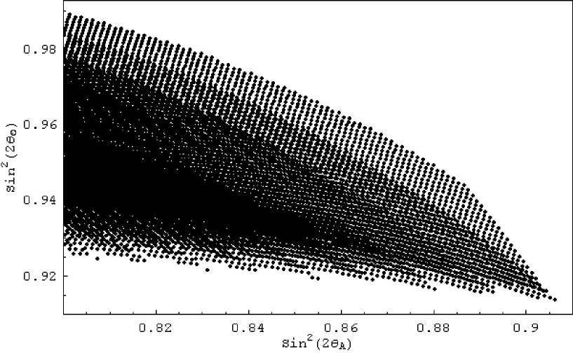
FIG. 1.: The figure shows the range of predictions for $\sin^{2}2\theta_{\odot}$ and $\sin^{2}2\theta_{A}$ for the range of quark masses in table I that fit the charged lepton spectrum and where all CP phases are set to zero. We required that the ratio $\Delta m^{2}_{\odot}/\Delta m^{2}_{A}\leq 0.05$. Note that $\sin^{2}2\theta_{\odot}\geq 0.9$ and $\sin^{2}2\theta_{A}\leq 0.9$.

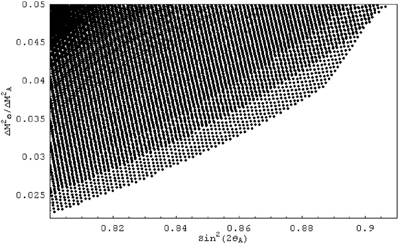
FIG. 2.: The figure shows the predictions for $\sin^{2}2\theta_{A}$ and $\Delta m^{2}_{\odot}/\Delta m^{2}_{A}$ for the range of quark masses and mixings that fit charged lepton masses and where all CP phases in the fermion masses are set to zero.

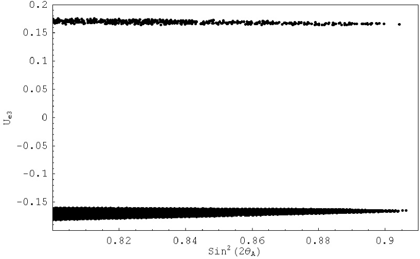
FIG. 3.: The figure shows the predictions of the model for $\sin^{2}2\theta_{A}$ and $U_{e3}$ for the allowed range of parameters in the model as in Fig. 1 and 2. Note that $U_{e3}$ is very close to the upper limit allowed by the existing reactor experiments.

V Effect of CP phases on neutrino mixings

In this section, we keep the CP phases as described before and look for solutions to the charged lepton equation, Eq. (17) and then use the allowed parameter range to look at the predictions of the neutrino masses and mixings. We have seven CP phases including the CKM phase. One might think that since there are more parameters in this case, getting a solution will be trivial. We find that actually, it is not so. Let us demonstrate this in an analytic way very crudely and we follow it up with detailed numerical scan to get the mixing angles.

To proceed with this analysis, first note that the phases are distributed in Eq. (17) as follows. First the down quark mass eigenvalues are chosen to be complex i.e. $(\tilde{m_{d}}e^{i\beta_{1}},\tilde{m_{s}}e^{i\beta_{2}},e^{i\beta_{3}})$ and similarly for the up quark sector, there are three phases in the masses (denoted by $\alpha_{i}$). Using 17, we see that

$$kM_{\ell} = \pmatrix{r\tilde{m_{d}}e^{i\beta_{1}}+\tilde{m_{c}}\lambda^{2}e^{i\alpha_{2}}&\tilde{m_{c}}\lambda e^{i\alpha_{2}}+A^{2}\lambda^{5}e^{i\alpha_{3}}(\Lambda)&A\tilde{m_{c}}\lambda^{3}e^{i\alpha_{2}}+A\lambda^{3}e^{i\alpha_{3}}(\Lambda)\cr+A^{2}\lambda^{6}e^{i\alpha_{3}}(\Lambda)^{2}&&\cr\tilde{m_{c}}\lambda e^{i\alpha_{2}}+A^{2}\lambda^{5}e^{i\alpha_{3}}(\Lambda)&r\tilde{m_{s}}e^{i\beta_{2}}+\tilde{m_{c}}e^{i\alpha_{2}}+A^{2}\lambda^{4}e^{i\alpha_{3}}&\tilde{m_{c}}A\lambda^{2}e^{i\alpha_{2}}+A\lambda^{2}e^{i\alpha_{3}}\cr&&\cr A\tilde{m_{c}}\lambda^{3}e^{i\alpha_{2}}+A\lambda^{3}e^{i\alpha_{3}}(\Lambda)&\tilde{m_{c}}A\lambda^{2}e^{i\alpha_{2}}+A\lambda^{2}e^{i\alpha_{3}}&re^{i\beta_{3}}+\tilde{m_{c}}A^{2}\lambda^{4}e^{i\alpha_{2}}+e^{i\alpha_{3}}}$$ (36)

where we have used the Wolfenstein parametrization for the CKM matrix. Essentially the eigenvalues of the matrix on the right hand side must match the charged lepton masses. Note that as in the case without the CP phase, this will require us to work only in a very limited range of the quark masses. Since now we have to align the phases with the known standard model CKM phase, the constraints are even tighter. The muon and tau masses come out quite easily as in the case without phases discussed in the previous section.

As in the CP conserving case, the mass of the electron requires fine tuning as can be seen by noting that the $11$ entry of $M_{\ell}$ is roughly of order $\lambda^{4}$ which is about 3 to 4 times the value required to give the correct electron mass. One must therefore have cancellation to get the correct $m_{e}$ . Before discussing the details of this cancellation, let us first look at the neutrino mass matrix, which looks as follows:

$${\cal M}_{\nu} = \pmatrix{0&0&zA\lambda^{3}(1-\rho-i\eta)e^{i\alpha_{3}}\cr 0&0.7y\lambda^{2}e^{\beta_{2}}&zA\lambda^{2}e^{i\alpha_{3}}\cr zA\lambda^{3}(1-\rho-i\eta)e^{i\alpha_{3}}&zA\lambda^{2}e^{i\alpha_{3}}&ye^{i\beta_{3}}-ze^{i\alpha_{3}}}$$ (37)

First thing to note is that we must have $\alpha_{3}=\beta_{3}$ for $b-\tau$ unification to lead to maximal mixing.

To see very qualitatively what value of CKM phase is required for the model to work, we need to analyze the charged lepton masses. As in the CP conserving case, the muon and the tau mass come out for the choice of $k\approx 0.25$ and $r\approx-.75$. Let us now discuss the electron mass. For this we first note that we use the Wolfenstein parametrization. The two parameters $\rho$ and $\eta$ responsible for the CKM phase are given by the latest data to be[21] $.12\leq\rho\leq.35$ and $0.28\leq\eta\leq.41$. Since the charged lepton mass matrix has hierarchical structure, we can deduce an approximate formula for $m_{e}$ from the sum rule 17 and using the above values of $k$ and $r$:

$$\tilde{m}_{e}\simeq-3\tilde{m_{d}}e^{i\beta_{1}}+\tilde{m_{c}}\lambda^{2}e^{i\alpha_{2}}+A^{2}\lambda^{6}e^{i\alpha_{3}}(\Lambda)^{2}-{(4A\lambda^{6}(1-\rho-i\eta)^{2}e^{i\alpha_{3}})}-O(\lambda^{7})$$ (38)

Numerically, to get the correct value for $\tilde{m}_{e}\simeq 0.00028\simeq 0.6\lambda^{5}$, we must cancel most of the $\tilde{m}_{d}$ contribution to it i.e. $-3\tilde{m}_{d}\simeq 1.3\lambda^{4}$, from the other terms: these terms get maximized for $\rho<0$ in which case we get $|1-\rho-i\eta|\simeq 1.41$ so that the last term contributes $32\lambda^{6}\simeq 1.5\lambda^{4}$. It also determines the arbitrary phases that accompany the quark masses as follows: $\beta_{1}=\alpha_{2}=\alpha_{3}+2\delta$ where $\tan\delta\simeq\frac{\eta}{1-\rho}$ and $m_{d}<0$. The terms in the electron mass formula then cancel leading to $\tilde{m}_{e}\simeq.9\lambda^{5}$ which is in the rough “neighborhood” of the observed value ($\tilde{m}_{e}$). This value of $\rho$ gives a CKM phase which is in the third quadrant implying that in order to understand the observed CP violation i.e. $\sin 2\beta$ in B-system, one will need to invoke CP violation from the supersymmetry breaking scalar masses.

Again we caution the reader that this is a crude estimate. In detailed numerical analysis, we can get solutions for small positive $\rho$ and one next has to see how these values fit the neutrino mixings. Thus combined fit to both electron mass and neutrino mixings works only for negative $\rho$ value which is different from the current standard model CKM fit.

The detailed numerical predictions for this model are given in Fig. 4,5 and 6, where we have scanned over all the phases looking for the correct charged lepton masses and acceptable neutrino parameters. We have also extended the domain of $\Delta m^{2}_{\odot}/\Delta m^{2}_{A}$ to $0.08$.

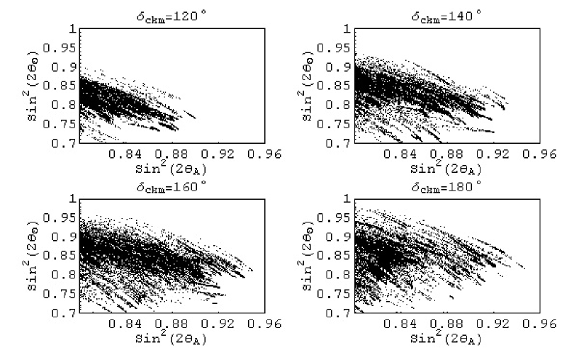
FIG. 4.: The figure shows the predictions for $\sin^{2}2\theta_{A}$ and $\sin^{2}2\theta_{\odot}$ for the range of quark masses and mixings that fit charged lepton masses in the presence of all CP phases in the fermion masses. The four different panels give the predictions for different values of the CKM phase ($\tan\delta_{CKM}=\frac{\eta}{\rho}$). Note that all these values are outside the one sigma region of the present standard model fit to all CP violating data. Note that the case $\delta_{CKM}=180$ includes the CP conserving case discussed in sec. IV.

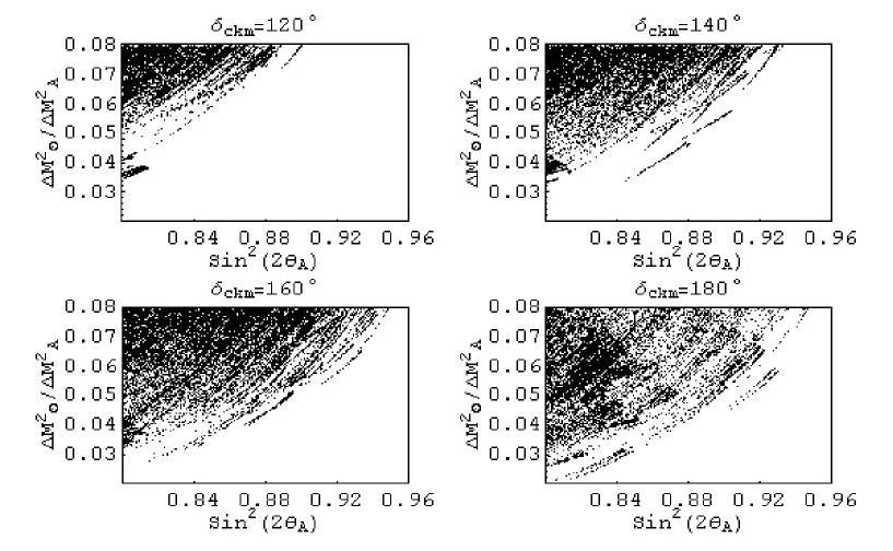
FIG. 5.: The figure shows the predictions for $\sin^{2}2\theta_{A}$ and $\Delta m^{2}_{\odot}/\Delta m^{2}_{A}$ for the range of quark masses and mixings that fit charged lepton masses and where all CP phases in the fermion masses are kept subject to the condition that b-tau mass convergence is responsible for large neutrino mixings, for four different values of the $\delta_{CKM}$.

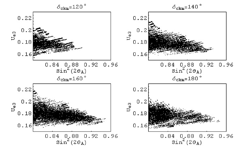
FIG. 6.: The figure shows the predictions for $\sin^{2}2\theta_{A}$ and $U_{e3}$ for the range of quark masses and mixings that fit charged lepton masses and where all CP phases in the fermion masses are included, for four different values of $\delta_{CKM}$.

In concluding this section, we note that since the main constraints on the model came from trying to fit the electron mass, it is worth pointing out that one way to avoid these constraints is to include the effects of the higher dimensional operators (HDO) which contribute to the electron mass and is too small to be of relevance in the discussion of other masses. Since usually the contribution of HDO terms in this theory would contribute terms of order $\left(\frac{M_{U}}{M_{P\ell}}\right)^{n}\simeq 10^{-2n}$, where $3+n$ denotes the dimensionality of the HDO. The leading order HDO must therefore correspond to $n=2$. This can be guaranteed for instance by demanding that superpotential is R-odd and all the Higgs fields are R-odd, whereas the matter fields are R-even. We have repeated our computations with the HDO terms mentioned and we find that one can obtain the neutrino mixing parameters in the right range for the standard model value of the CKM phase.

A CP violation in leptonic mixings

The neutrino mass matrix discussed above can be approximately diagonalized to obtain the CP phases in the PMNS matrix. For this purpose, we first diagonalize the charged lepton mass matrix. The mixing matrix has a form similar to the CKM matrix. Therefore, in the basis where charged leptons are mass eigenstates, the neutrino mass matrix remains approximately of the same form as in Eq. (23) i.e.

$${\cal M}_{\nu} = m_{0}zA\lambda^{2}\pmatrix{0&0&ae^{i(\delta+\alpha_{3})}\cr 0&(1+\epsilon)e^{i\beta_{2}}&e^{i\alpha_{3}}\cr ae^{i(\delta+\alpha_{3})}&e^{i\alpha_{3}}&\frac{(ye^{i\beta_{3}}-ze^{i\alpha_{3}})}{zA\lambda^{2}}}$$ (39)

where $a=\sqrt{(1\pm\rho)^{2}+\eta^{2}}~{}zA\lambda$; $\epsilon~{}\simeq\frac{0.7y}{z}-1$ and $\tan\delta\simeq\frac{\eta}{1-\rho}$ . In the expression for $a$ and $\tan\delta$, the plus sign corresponds to the case without any contribution from the higher dimension terms to the electron mass and the minus corresponds to the case with higher dimensional terms. In order to get maximal mixing out of b-tau mass convergence, we must have $\alpha_{3}=\beta_{3}$ and $(ye^{i\beta_{3}}-ze^{i\alpha_{3}})\simeq zA\lambda^{2}$. Furthermore, to get the solar mass difference right, we must have $\beta_{2}=\alpha_{3}$. We can therefore take the common phase $e^{i\alpha_{3}}$ out of the matrix which leaves us with a simple matrix of the form

$$\tilde{{\cal M}}_{\nu} = \pmatrix{0&0&ae^{i\delta}\cr 0&(1+\epsilon)&1\cr ae^{i\delta}&1&1}$$ (40)

diagonalize. The matrix that diagonalizes it is of the form

$${\bf U}~{}=~{}V\left(\begin{array}[]{ccc}c&-s&{a\over 2}\sqrt{2}\\ -\frac{(s(1-{\epsilon\over 4})+c\sqrt{2}{a\over 4})}{\sqrt{2}}&\frac{(-c(1-{\epsilon\over 4})+s\sqrt{2}{a\over 4})}{\sqrt{2}}&\frac{1+{\epsilon\over 4}}{\sqrt{2}}\\ \frac{(s(1+{\epsilon\over 4})-c\sqrt{2}{a\over 4})}{\sqrt{2}}&\frac{(c(1+{\epsilon\over 4})+s\sqrt{2}{a\over 4})}{\sqrt{2}}&\frac{1}{\sqrt{2}}\end{array}\right)$$ (44)

where ${\bf V}~{}=~{}diag(e^{i\delta},1,1)$. Note that since the PMNS mixing matrix is real to order $\lambda$, direct CP violating effects among neutrinos are suppressed and unobservable in near future. This is a definite prediction of the minimal SO(10) model. In a sense this is not surprising, since the lepton sector and the quark sector are linked by quark-lepton unification and we know that in the quark sector the CP violating phase is only present in the $\lambda^{3}$ order.

Since the model predicts a large $U_{e3}$, if there is any CP violating phase in the mixing matrix, it has a better chance of being observable; on the other hand this model predicts no CP violation, so that the model has a better chance of being falsifiable and strengthens the case for searching for CP violation in neutrino oscillations. It is important to emphasize that the model however enough CP violation to in the right handed neutrino couplings so that one should expect enough baryogenesis.

VI Summary and conclusions

In summary, we have shown that the minimal SO(10) model with fermion masses receiving contributions from only one 10 and one 126 Higgs multiplets is fully predictive in the neutrino sector. It predicts all three neutrino mixing angles in agreement with present data but with a value of $U_{e3}$ which is very close to the present upper limits from the reactor experiments. This high value of $U_{e3}$ provides a test of the model. We also find that the introduction of CP phases in the Yukawa couplings still keeps the model predictive. The CKM phase in this case is outside the one $\sigma$ region of the present central value in the standard model suggesting that there are new CP violating contributions from the SUSY breaking sector. We find it interesting that to the leading order in the Cabibbo angle, the leptonic CP violation vanishes in spite of the fact that the quark sector has CP violation.

There are no additional global symmetries assumed in the analysis. The neutrino data once refined would therefore provide a crucial test of minimal SUSY SO(10) in the same way as proton decay was considered a crucial test of minimal SU(5).

This work is supported by the National Science Foundation Grant No. PHY-0099544.

REFERENCES

- [1] J. Bahcall, C. Gonzalez-Garcia and C. Pena-Garay, hep-ph/0204314; V. Barger, K. Whisnant, D. Marfatia and B. P. Wood, hep-ph/0204253; A. Bandopadhyay, S. Choubey, S. Goswami and D. P. Roy, hep-ph/0204286; P. de Holanda and A. Smirnov, hep-ph/0205241; M. Maltoni, T. Schwetz, M. Tortola and J. W. F. Valle, hep-ph/0207227; G. Fogli, E. Lisi, A. Marrone and D. Montanino, hep-ph/0212127; hep-ph/0303064; G. Fogli et al. hep-ph/0208026;
- [2] For recent reviews, see S. Bilenky, C. Giunti, J. Grifols and E. Masso, hep-ph/0211462 (Phys. Rep., to appear); C. Gonzalez-Garcia and Y. Nir, hep-ph/0202058; V. Barger, D. Marfatia and K. Whisnant, hep-ph/hep-ph/0308123.
- [3] R. N. Mohapatra, hep-ph/0211252; G. Altarelli and F. Feruglio, hep-ph/0306265; Z. Z. Xing, hep-ph/0307359.
- [4] M. Gell-Mann, P. Rammond and R. Slansky, in Supergravity, eds. D. Freedman et al. (North-Holland, Amsterdam, 1980); T. Yanagida, in proc. KEK workshop, 1979 (unpublished); R.N. Mohapatra and G. Senjanović, Phys. Rev. Lett. 44, 912 (1980); S. L. Glashow, Cargese lectures, (1979).
- [5] R. N. Mohapatra and R. E. Marshak, Phys. Rev. Lett. 44, 1316 (1980).
- [6] Y. Chikashige, R. N. Mohapatra and R. D. Peccei, Phys. Lett. 98 B, 265 (1981).
- [7] H. Georgi, in Particles and Fields (ed. C. E. Carlson), A. I. P. (1975); H. Fritzsch and P. Minkowski, Ann. of Physics, Ann. Phys. 93, 193 (1975).
- [8] R N Mohapatra: Phys. Rev. 34, 3457 (1986); A. Font, L. Ibanez and F. Quevedo, Phys. Lett. B228, 79 (1989); S. P. Martin, Phys. Rev. D46, 2769 (1992).
- [9] K. S. Babu and R. N. Mohapatra, Phys. Rev. Lett. 70, 2845 (1993).
- [10] D. G. Lee and R. N. Mohapatra, Phys. Rev. D 51, 1353 (1995).
- [11] C. S. Aulakh, A. Melfo, A. Rasin, G. Senjanovic, Phys. Lett. B 459, 557 (1999); C. S. Aulakh, B. Bajc, A. Melfo, A. Rasin, G. Senjanovic, hep-ph/0004031.
- [12] K. S. Babu, J. C. Pati and F. Wilczek, hep-ph/9812538, Nucl. Phys. B566, 33 (2000); C. Albright and S. M. Barr, Phys. Rev. Lett. 85, 244 (2001); T. Blazek, S. Raby and K. Tobe, Phys. Rev. D62, 055001 (2000); M. C. Chen and K. T. Mahanthappa, Phys. Rev. D 62, 113007 (2000); Z. Berezhiani and A. Rossi, Nucl. Phys. B594, 113 (2001); R. Kitano and Y. Mimura, Phys. Rev. D63, 016008 (2001); for a recent review, see C. Albright, hep-ph/0212090.
- [13] L. Lavoura, Phys. Rev. D48 5440 (1993).
- [14] B. Brahmachari and R. N. Mohapatra, Phys. Rev. D58, 015003 (1998).
- [15] K. Oda, E. Takasugi, M. Tanaka and M. Yoshimura, Phys. Rev. D59, 055001 (1999).
- [16] T. Fukuyama and N. Okada, hep-ph/0206118; T. Fukuyama, Y. Koide, K. Matsuda and H. Nishiura, Phys. Rev. D 65, 033008 (2002).
- [17] M. C. Chen and K. T. Mahanthappa, Phys.Rev. D62, 113007 (2000); Y. Achiman and W. Greiner, Phys. Lett. B 329, 33 (1994).
- [18] R. N. Mohapatra and G. Senjanović, Phys. Rev. D 23, 165 (1981); C. Wetterich, Nuc. Phys. B 187, 343 (1981); G. Lazarides, Q. Shafi and C. Wetterich, Nucl.Phys.B181, 287 (1981); E. Ma and U. Sarkar, Phys. Rev. Lett. 80, 5716 (1998).
- [19] B. Bajc, G. Senjanović and F. Vissani, hep-ph/0210207.
- [20] H. S. Goh, R. N. Mohapatra and S.-P. Ng, hep-ph/0303055.
- [21] For a review, see Y. Nir, hep-ph/0208080.
- [22] C. S.Aulakh and R. N. Mohapatra, Phys. Rev. D 28, 217 (1983); D. Chang, R. N. Mohapatra and M. K. Parida, Phys. Rev. D 30, 1052 (1984); J. Baseq, S. Meljanac and L. O’Raifeartaigh, Phys. Rev. D 39, 3110 (1989); D. G. Lee, Phys. Rev. D 49, 1417 (1994); C. S. Aulakh, A. Melfo, B. Bajc, G. Senjanović and F. Vissani, hep-ph/0306242.
- [23] D. Chang and R. N. Mohapatra, Phys. Rev. D 32, 1248 (1985).
- [24] Similar mass matrices with small parameters have been discussed, for example, in G. Altarelli and F. Feruglio, Phys.Lett. B439, 112 (1998); R. N. Mohapatra and S. Nussinov, Phys.Rev. D60, 013002 (1999) E. Akhmedov, G. Branco and M. N. Rebelo, Phys. Lett. B 478, 215 (2000); A. Yu Smirnov and M. Frigerio, hep-ph/0207366; for a review and other references, see [3].
- [25] see for instance, V. Barger, M. Berger and P. Ohmann, Phys. Rev. D47, 333 (1993); S. Naculich, Phys. Rev. D48, 5293 (1993); H. Fusaoka and Y. Koide, Phys. Rev. D64, 053014 (2001); M. K. Parida and B. Purkayastha, Eur. Phys. J. C14, 159 (2000); C. R. Das and M. K. Parida, hep-ph/0010004; Eur. Phys. J. C20, 121 (2001).
- [26] For a review, see K. Scholberg, hep-ex/0308011.
- [27] For a review, see A. Smirnov, hep-ph/0306075; J. Bhacall and C. Pena-Garay, hep-ph/0305159.
- [28] M. Szeleper and A. Para, hep-ex/0110032; M. Diwan et al. BNL-69395 (2002).
- [29] Y. Itow et al. (JHF Collaboration), hep-ex/0106019.