Phenomenology of low-scale supersymmetry breaking models

In this letter we consider the distinctive phenomenology of supersymmetric models in which the scale of SUSY breaking is very low, $\sqrt{F}={\cal O}(\rm TeV)$, focusing on the Higgs sector and the process of electroweak breaking. Using an effective Lagrangian description of the interactions between the observable fields and the SUSY breaking sector, it is shown how the conventional MSSM picture can be substantially modified. For instance, the Higgs potential has non-negligible SUSY breaking quartic couplings that can modify completely the pattern of electroweak breaking and the Higgs spectrum with respect to that of conventional MSSM-like models.

IPPP/03/40

DCPT/03/92

1 Introduction

Supersymmetry (SUSY), despite all the new, recently proposed solutions to the gauge hierarchy problem, is still (probably) the best candidate for new physics above the electroweak scale. The fact that it can stabilize “tree level” mass scales against radiative corrections, thus solving the gauge hierarchy problem, is its more appreciated feature, but it has many other (good) characteristics. It is not free, however, of phenomenological and theoretical problems (for reviews, see [1]). Almost all of them are related to the fact that SUSY, if realized in nature, has to be broken. The way this breaking takes place is usually the more obscure point of supersymmetric models. In any case, it is encouraging (and non-trivial) that one can build phenomenologically viable models in which SUSY is broken, all scalar partners of Standard Model (SM) fermions acquire a positive mass squared and the electroweak breaking takes place in a satisfactory way.

The usual approach in phenomenological studies of supersymmetric models is to write down a supersymmetric Lagrangian and to supplement it with a set of supersymmetry breaking (SUSY) terms that parameterize the effect of the breaking, without making any assumption about the nature of the breaking itself. The only thing that is required is that these terms do not generate quadratic divergences in the renormalization of scalar masses (therefore they are called $soft$ terms). However, when doing this, we $are$ making an assumption about the nature of the SUSY: we are assuming that the breaking takes place at a very high energy scale. The reason for this is the following. Suppose SUSY is broken in some sector of the theory in which there are some fields whose F-terms take some vacuum expectation value (v.e.v.), of order $F$. This breaking will be transmitted to every other sector of the theory. The scalar SUSY breaking masses in any other sector (coupled to this one only through interactions suppressed by powers of some mass scale $M$) are typically of order $m_{s}\sim F/M$. However, the appearance of $soft$ breaking terms is not the only effect of the breaking, since the so-called $hard$ breaking terms are also generated. For instance, SUSY quartic couplings for the scalars are typically of order $\lambda_{h}\sim m_{s}^{2}/M^{2}$ [2, 3]. These hard breaking terms are always suppressed by inverse powers of $M$ with respect to the soft terms, so in the case of a big hierarchy $M\gg\sqrt{F}\gg m_{s}$, neglecting this terms makes a good approximation. However, although in most models of SUSY there is in fact a hierarchy in the scales involved, we have no real information available about what these scales are, and for all that we know they could be of order $TeV$.

In this letter, following [3], we will review the (quite distinctive) phenomenological properties of theories in which all these scales are of order $TeV$, so the hard SUSY terms play a relevant role in the phenomenology. Notice that these terms, although $do$ generate quadratic divergencies in the renormalization of scalar masses, $do$ $not$ destabilize any hierarchy since they are suppressed by powers of the mass scale $M$, that is to be identified with the cut-off of the effective description of SUSY that we are considering. Actually, the fact that SUSY protects mass scales against radiative corrections is not due to the absence of quadratic divergences in the quantum corrections to the theory, since in fact there are quadratic divergences in its quantum corrections (see [4] for compact formulae encoding all one loop radiative corrections to a general 4D $N=1$ SUSY theory). The reason why mass scales are stabilized against quantum corrections can be traced back to the fact that all radiative corrections can be incorporated to the Kähler potential, since we know from non-renormalization theorems that the superpotential is not renormalized in perturbation theory. Since the Kähler potential is a real function of the fields with mass dimension two, the only $relevant$ operator ($i.e.$ the only term in which a positive mass dimension coupling could appear, so that quantum corrections could drive it to be of the order of the cut-off) would be one with a single field, that should be a singlet $\delta K\sim XS$, with $S$ a singlet and $X$ a parameter with dimensions of mass that would naturally be of the order of the cut-off. However, in global SUSY such terms in the Kähler potential are not meaningful since they do not give any contribution to the Lagrangian, so quantum corrections will never destabilize mass scales in global SUSY.

In this brief review, we will focus on the low energy phenomenology and we will pay particular attention to the interplay of SUSY and electroweak breaking and to the Higgs sector spectrum in low scale SUSY models. New possibilities for electroweak breaking show up [3], this breaking generically takes place in a less fine tuned way [6] and the lightest Higgs boson can be much heavier than in conventional MSSM scenarios [2, 3]. Another important feature of these scenarios is that the gravitino is superlight (with a mass $m_{3/2}=F/(\sqrt{3}M_{p}$)), and its couplings with MSSM fields are in general not suppressed, so one can find characteristic collider signatures of such a superlight gravitino [7] (see [8] for other phenomenological implications of a superlight gravitino).

2 Supersymmetry breaking: effective description.

Almost all models that try to address the problem of how SUSY is transmitted to the observable sector share a common structure: it is assumed that SUSY is broken in some “hidden” sector, at a scale $F$, and that this sector couples to the MSSM fields only trough non-renormalizable interactions suppressed by powers of some high energy mass scale $M$. Different models propose different physics generating these effective interactions. For instance, in gravity mediation these are the interactions generated by the structure of the supergravity Lagrangian, and thus this scale is the Planck mass, $M=M_{p}$. Fixing $m_{s}\sim F/M_{p}$ to be of order $TeV$ to solve the hierarchy problem we get $\sqrt{F}$ to be ${\cal O}(10^{11}GeV)$. Another example is gauge mediation, where it is assumed that there are some fields charged under the SM gauge group that couple at tree level to the SUSY sector. If these fields have a large mass $M$, below this mass we get an effective theory in which the MSSM fields are coupled to the SUSY sector through non-renormalizable interactions (generated at the loop level) suppressed by powers of $M$.

Generically, the specific details of the mediation mechanism generate specific patterns of soft breaking terms. It is not a coincidence that all these models have this common structure. The reason for this is that if one tries to break supersymmetry in a renormalizable model one finds that the supertrace of the mass matrix is identically zero even when SUSY is broken. This means that the sum of the masses of fermions is equal to the sum of the masses of bosons. So if we try to break supersymmetry using only the MSSM fields and a renormalizable Lagrangian we will always find superparticles lighter than some ordinary particles. This difficulties are overcome in models in which the transmission of SUSY to MSSM particles can be described using an effective non-renormalizable Lagrangian (that is valid only up to some high energy scale $M$). In this spirit, the approach that we will follow is to describe the transmission of SUSY using effective interactions, without relying on any specific microscopic dynamics that can generate it. This new physics should be now close to the electroweak scale and it could be some massive fields (analogously to the case of gauge mediation), or could have a more fundamental character, as in supersymmetric models with a low scale of quantum gravity, see for instance [9]. This scale of new physics, although close to the electroweak scale, still has to be somewhat larger than it, so it makes sense to consider the effective theory below it, (but above the electroweak scale). We will assume that after integrating out these heavy degrees of freedom we are left with a globally supersymmetric theory whose degrees of freedom are just those of the MSSM plus a singlet chiral superfield, $T$, responsible of SUSY .

Our starting point will be the $N$=1 globally supersymmetric Lagrangian

$${\cal L}=\int\!\!d^{4}\theta K(\bar{\phi},e^{2V}\phi)+\left[\int\!\!d^{2}\theta\,W(\phi)+{\rm h.c.}\right]+{1\over 4}\left[\int\!\!d^{2}\theta f_{ab}(\phi){\cal W}^{a}{\cal W}^{b}+{\rm h.c.}\right]$$ (1)

where $K(\bar{\phi},\phi)$, $W(\phi)$ and $f_{ab}(\phi)$ are the effective Kähler potential, superpotential and gauge kinetic functions, respectively, and higher derivative terms are neglected. We decompose chiral superfields according to $\phi^{i}\Rightarrow\phi^{i}+\sqrt{2}\psi^{i}\theta+F^{i}\theta\theta+\ldots$ and vector superfields according to $V^{a}\Rightarrow A^{a}_{\mu}\theta\sigma^{\mu}\bar{\theta}+(\lambda^{a}\theta\bar{\theta}\bar{\theta}+{\rm h.c.})+{1\over 2}D^{a}\theta\theta\bar{\theta}\bar{\theta}$, in the Wess-Zumino gauge. The effective Lagrangian for the component fields can be obtained by a standard procedure [10] (see also the appendix of [9]). In particular, the scalar potential has the general expression

$$V=V_{F}+V_{D}=W_{i}K^{i\bar{\jmath}}\bar{W}_{\bar{\jmath}}\ +\ {1\over 2}\left[K_{i}({\bf t}_{a}\phi)^{i}+\xi_{a}\right]f_{R}^{ab}\left[K_{j}({\bf t}_{b}\phi)^{j}+\xi_{b}\right]\,.$$ (2)

Subscripts denote derivatives ($W_{i}\equiv\partial W/\partial\phi^{i}$, $\bar{W}_{\bar{\jmath}}\equiv\partial{\bar{W}}/\partial\bar{\phi}^{\bar{\jmath}}\equiv(\partial W/\partial\phi^{j})^{*}$, $K_{i}\equiv\partial K/\partial\phi^{i}$,…), $K^{i\bar{\jmath}}$ is the inverse of the Kähler metric $K_{\bar{\imath}j}\equiv\partial^{2}K/\partial\bar{\phi}^{\bar{\imath}}\partial\phi^{j}$ and $f_{R}^{ab}$ is the inverse of the metric $(f_{R})_{ab}\equiv{\rm Re}f_{ab}$ of the vector sector (i.e. $K^{i\bar{\jmath}}K_{\bar{\jmath}\ell}=\delta^{i}_{\ell}$ and $f_{R}^{ab}(f_{R})_{bc}=\delta^{a}_{c}$). The order parameter for supersymmetry breaking, which will be non-zero by assumption, is

$$F^{2}\equiv\langle V\rangle=\langle V_{F}+V_{D}\rangle=\langle{\bar{F}}^{\bar{\imath}}K_{\bar{\imath}j}F^{j}+{1\over 2}D^{a}(f_{R})_{ab}D^{b}\rangle\,,$$ (3)

where the v.e.v.s of the auxiliary fields are

$$\langle F^{i}\rangle=-\langle K^{i\bar{\jmath}}\bar{W}_{\bar{\jmath}}\rangle\;\;,\;\;\langle D^{a}\rangle=-\langle f_{R}^{ab}\left[K_{j}({\bf t}_{b}\phi)^{j}+\xi_{b}\right]\rangle\ .$$ (4)

Fermion mass terms have the form $-{1\over 2}(\lambda^{a},\psi^{i}){\cal M}(\lambda^{b},\psi^{j})^{T}+{\rm h.c.}$, where the matrix ${\cal M}$ is given by

$${\cal M}=\left(\begin{array}[]{cc}-\displaystyle{1\over 2}\langle(f_{ab})_{\ell}F^{\ell}\rangle&\sqrt{2}\langle K_{\bar{\ell}j}(\overline{{\bf t}_{a}\phi})^{\bar{\ell}}+\displaystyle{1\over 4}(f_{ac})_{j}D^{c}\rangle\\ &\\ \sqrt{2}\langle K_{\bar{\ell}i}(\overline{{\bf t}_{b}\phi})^{\bar{\ell}}+\displaystyle{1\over 4}(f_{bc})_{i}D^{c}\rangle&\langle W_{ij}+{\bar{F}}^{\bar{\ell}}K_{\bar{\ell}ij}\rangle\end{array}\right)\ .$$ (5)

By using the extremum conditions of the scalar potential and gauge invariance, it is easy to check that the mass matrix ${\cal M}$ has an eigenvector $({1\over\sqrt{2}}\langle D^{b}\rangle,\langle F^{j}\rangle)^{T}$ with zero eigenvalue, which corresponds to the goldstino state. This eigenvector specifies the components of goldstino field $\tilde{G}$ contained in the original fields $\psi^{i}$ and $\lambda^{a}$. We also recall that, in the framework of local SUSY, the goldstino degrees of freedom become the longitudinal components of the gravitino, which obtains a mass $m_{3/2}=F/(\sqrt{3}M_{p})$. When $\sqrt{F}$ is close to the electroweak scale, $m_{3/2}$ is much smaller than typical experimental energies, which implies that the dominant gravitino components are precisely the goldstino ones [11].

The chiral superfields will be denoted by $\phi^{i}=(\phi^{\alpha},T)$, where $\phi^{\alpha}$ are the MSSM chiral superfields (containing Higgses, leptons and quarks) and $T$ is the singlet superfield whose auxiliary field v.e.v. $\langle F^{T}\rangle$ breaks SUSY. For small fluctuations of the fields $\phi^{\alpha}$, the expansions of $K$, $W$ and $f_{ab}$ can be written as

$$K = k(\bar{T},T)+c_{\bar{\alpha}\beta}(\bar{T},T)\bar{\phi}^{\bar{\alpha}}\phi^{\beta}+{1\over 2}\left[d_{\alpha\beta}(\bar{T},T)\phi^{\alpha}\phi^{\beta}+{\rm h.c.}\right]+\ldots$$ (6)

$$W = w(T)+{1\over 2}\mu_{\alpha\beta}(T)\phi^{\alpha}\phi^{\beta}+{1\over 3!}h_{\alpha\beta\gamma}(T)\phi^{\alpha}\phi^{\beta}\phi^{\gamma}+\ldots$$ (7)

$$f_{ab} = f_{a}(T)\delta_{ab}+\ldots$$ (8)

The functions $c_{\bar{\alpha}\beta},d_{\alpha\beta},h_{\alpha\beta\gamma},f_{a}$ are assumed to depend on $T$ through the ratio $T/M$, where $M$ is the typical scale of suppression of the non-renormalizable operators of the theory. This theory is therefore an effective description of some yet more fundamental theory, and is valid only up to this scale, $M$. Then the induced SUSY-breaking mass splittings within the $\phi^{\alpha}$ and $V^{a}$ multiplets are characterized by a scale $\tilde{m}\sim F/M$. We also make the standard assumption that $\mu_{\alpha\beta}$, if non-vanishing, has size ${\cal O}(\tilde{m})$ rather than ${\cal O}(M)$, i.e. $\mu_{\alpha\beta}(T)\sim(F/M){\tilde{\mu}}_{\alpha\beta}(T/M)$.

As we said, standard scenarios are characterized by a strong hierarchy $M\gg\sqrt{F}\gg\tilde{m}$. In this limit the physical components of the $T$ multiplet (i.e. the goldstino and its scalar partners, the ‘sgoldstinos’) are almost decoupled from the other fields, and the effective theory for the $\phi^{\alpha}$ and $V^{a}$ multiplets is well approximated by a renormalizable one. The latter is characterized by gauge couplings $g_{a}^{2}=1/\langle{\rm Re}f_{a}\rangle_{0}$, an effective superpotential $\hat{W}$ and a set of soft SUSY breaking terms, whose mass parameters are ${\cal O}(\tilde{m})$. This is the usual MSSM scenario. The MSSM parameters can be computed in terms of the functions appearing in $K$, $W$ and $f_{ab}$ above. Let us consider for simplicity the case of diagonal matter metric, i.e. $c_{\bar{\alpha}\beta}=c_{\alpha}\delta_{\bar{\alpha}\beta}$, and rescale the fields in order to have canonical normalization: $\langle\sqrt{c_{\alpha}}\rangle_{0}\phi^{\alpha}\rightarrow\phi^{\alpha}$, $\langle\sqrt{{\rm Re}f_{a}}\rangle_{0}V^{a}\rightarrow V^{a}$. The effective superpotential of the renormalizable theory is

$$\hat{W}={1\over 2}\hat{\mu}_{\alpha\beta}\phi^{\alpha}\phi^{\beta}+{1\over 3!}\hat{h}_{\alpha\beta\gamma}\phi^{\alpha}\phi^{\beta}\phi^{\gamma}\ ,$$ (9)

where

$$\hat{\mu}_{\alpha\beta} = \left\langle\frac{\mu_{\alpha\beta}+\bar{F}^{\bar{T}}\partial_{\bar{T}}d_{\alpha\beta}}{(c_{\alpha}c_{\beta})^{1/2}}\right\rangle_{0}\ ,$$ (10)

$$\hat{h}_{\alpha\beta\gamma} = \left\langle\frac{h_{\alpha\beta\gamma}}{(c_{\alpha}c_{\beta}c_{\gamma})^{1/2}}\right\rangle_{0}\ .$$ (11)

Soft breaking terms are described by

$${\cal L}_{\rm soft}=-\tilde{m}_{\alpha}^{2}|\phi^{\alpha}|^{2}-\left[{1\over 2}(\hat{\mu}_{\alpha\beta}B_{\alpha\beta})\phi^{\alpha}\phi^{\beta}+{1\over 3!}(\hat{h}_{\alpha\beta\gamma}A_{\alpha\beta\gamma})\phi^{\alpha}\phi^{\beta}\phi^{\gamma}+{1\over 2}M_{a}\lambda^{a}\lambda^{a}+{\rm h.c.}\right],$$ (12)

where

$$\tilde{m}_{\alpha}^{2} = \left\langle-|F^{T}|^{2}\partial_{T}\partial_{\bar{T}}\log c_{\alpha}\right\rangle_{0}\ ,$$ (13)

$$B_{\alpha\beta} = \left\langle-F^{T}\partial_{T}\log\left(\frac{\mu_{\alpha\beta}+\bar{F}^{\bar{T}}\partial_{\bar{T}}d_{\alpha\beta}}{c_{\alpha}c_{\beta}}\right)\right\rangle_{0}\ ,$$ (14)

$$A_{\alpha\beta\gamma} = \left\langle-F^{T}\partial_{T}\log\left(\frac{h_{\alpha\beta\gamma}}{c_{\alpha}c_{\beta}c_{\gamma}}\right)\right\rangle_{0}\ ,$$ (15)

$$M_{a} = \left\langle-F^{T}\partial_{T}\log({\rm Re}f_{a})\right\rangle_{0}\ .$$ (16)

The formulae presented above can be obtained also taking a specific limit ($M_{p}\rightarrow\infty$, $m_{3/2}\rightarrow 0$ with $F=\sqrt{3}m_{3/2}M_{p}$ fixed) of supergravity results [12].

In the case of strong hierarchy of scales these are all the SUSY effects one needs to consider at low energies. The $T$ multiplet has plays an external role in the derivation: it only provides the SUSY breaking v.e.v. $\langle F^{T}\rangle$. However, if the scales $M$ and $F$ are not much larger than the TeV scale and the ratio $F/M^{2}\sim\tilde{m}/M\sim\tilde{m}^{2}/F$ is not negligible, the standard MSSM picture is corrected by additional effects and novel features emerge. The components of MSSM multiplets ($\phi^{\alpha}$ and $V^{a}$) have novel non-negligible interactions among themselves as well as non-negligible interactions with the physical components of $T$ (goldstino and sgoldstinos). Moreover, since some of the $\phi^{\alpha}$ fields (i.e. the Higgses) have to obtain a v.e.v. in order to break the gauge symmetry, in principle one should reconsider the minimization of the scalar potential taking into account both $T$ and such fields. In addition, the $F$ components of the Higgs multiplets and the $D$ components of the neutral vector multiplets could give non-negligible contributions to SUSY breaking. In this case the goldstino could have components along all neutral fermions ($\tilde{T}$, Higgsinos and gauginos).

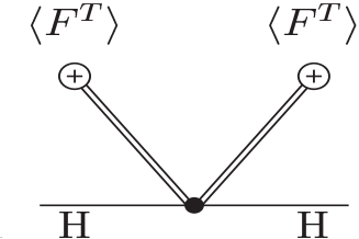
Figure 1: Diagramatic origin of the soft mass for the Higgses.

To see the origin of these hard breaking terms consider for instance a coupling $\delta K=-{\alpha\over M^{2}}|T|^{2}|H|^{2}$ in the Kähler potential. This term will give a contribution to the soft mass of the field $H$ (once the F-term of $T$ takes a v.e.v.) given by $\alpha m_{s}^{2}$ where $m_{s}^{2}\equiv\langle|F^{T}|^{2}\rangle/M^{2}$ as can be seen from eq.(13). One can visualize this contribution as coming from the diagram depicted in Fig. 1, where double lines represent auxiliary fields and crossed circles represent the v.e.v. $\langle F^{T}\rangle_{0}$. However, this term will also give contributions to a quartic coupling for $H$ coming from the diagram depicted in Fig. 2. So the total SUSY contribution to the potential of $H$ coming from such a term in the Kähler potential will be

$$\delta{\cal L}=\alpha\;m_{s}^{2}|H|^{2}+{2\alpha^{2}m_{s}^{2}\over M^{2}}|H|^{4}+\dots$$ (17)

where the dots represent higher order non-renormalizable terms. As for the case of the soft terms one can compute and give analytic expressions for all the SUSY terms that will be generated in the Lagrangian for the general theory with arbitrary $K$, $W$ and $f_{ab}$ that we are considering. We will focus now on the Higgs sector and discuss how these terms can modify significantly the pattern of electroweak breaking.

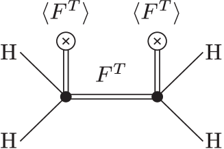
Figure 2: Diagramatic origin of quartic SUSY breaking couplings for the Higgses.

3 Electroweak breaking in low-scale supersymmetry breaking models.

When $F/M^{2}$ is not negligible, some higher order terms in the expansions of $K$, $W$ and $f_{ab}$ not written explicitly in eqs. (6), (7) and (8) can become important. In order to find all the possible renormalizable terms that can appear in the Higgs potential we will have to consider all the ${\cal O}(H^{4})$ terms in $W$ and $K$. As anticipated in the previous section, the coefficient functions appearing in $W$ and $K$ will depend on the field $T$ and on some mass scales. Thus we write:

$$W = w(T)+\mu(T)H_{1}\cdot H_{2}+{1\over 2M}\ell(T)\left(H_{1}\cdot H_{2}\right)^{2}+\ldots$$ (18)

$$K = k(\bar{T},T)+c_{1}(\bar{T},T)|H_{1}|^{2}+c_{2}(\bar{T},T)|H_{2}|^{2}+\left[d(\bar{T},T)H_{1}\cdot H_{2}+{\rm h.c.}\right]$$ (19)

$$+ {1\over 2M^{2}}e_{1}(\bar{T},T)|H_{1}|^{4}+{1\over 2M^{2}}e_{2}(\bar{T},T)|H_{2}|^{4}+{1\over M^{2}}e_{3}(\bar{T},T)|H_{1}|^{2}|H_{2}|^{2}$$

$$+ {1\over M^{2}}e_{4}(\bar{T},T)|H_{1}\cdot H_{2}|^{2}+\left[{1\over 2M^{2}}e_{5}(\bar{T},T)(H_{1}\cdot H_{2})^{2}\right.$$

$$+ \left.{1\over M^{2}}e_{6}(\bar{T},T)|H_{1}|^{2}H_{1}\cdot H_{2}+{1\over M^{2}}e_{7}(\bar{T},T)|H_{2}|^{2}H_{1}\cdot H_{2}+{\rm h.c.}\right]+\ldots$$

The Kähler potential $K$ is assumed to contain a single mass scale $M$. Thus the coefficient functions $c_{i}$, $d$ and $e_{i}$ in $K$ are in fact dimensionless functions of $T/M$ and $\bar{T}/M$ while $k(\bar{T},T)\sim M^{2}\tilde{k}(\bar{T}/M,T/M)$. On the other hand, $W$ should contain, besides $M$, the SUSY-breaking scale $F$ (notice that $F\sim\langle\partial_{T}W\rangle$). Although in our effective field theory approach it is not possible to determine what is the precise dependence on $M$ and $F$ of the coefficient functions in $W$, a reasonable criterion is to insure that each parameter of the component Lagrangian in the $T$-$H_{1}$-$H_{2}$ sector receives contributions of the same order from $K$ and $W$. An example of this are the two contributions to the effective $\hat{\mu}$ parameter in Eq. (10). The plausibility of this criterion is stressed by the fact that there is a considerable freedom to move terms between $K$ and $W$ through analytical redefinitions of the superfields. Consequently, we can assume

$$w(T)\sim FM\tilde{w}(T/M)\ ,\;\;\mu(T)\sim{F\over M}\tilde{\mu}(T/M)\ ,\;\;\ell(T)\sim{F\over M^{2}}\tilde{\ell}(T/M)\ ,$$ (20)

where $\tilde{w},\tilde{\mu},\tilde{\ell}$ are dimensionless functions of their arguments. For the expansion of the gauge kinetic functions $f_{ab}$ it is enough for our purpose to keep ${\cal O}(H^{2})$ terms. The indices in $f_{ab}$ are saturated with those of the super-field-strengths ${\cal W}^{a}{\cal W}^{b}$, see eq. (1), so the allowed irreducible representations in $f_{ab}$ are those contained in the symmetric product of two adjoints. For the $SU(2)\times U(1)$ gauge group, such representations are singlet, triplet and fiveplet:

$$f_{ab}=f^{(s)}_{ab}+f^{(t)}_{ab}+f^{(f)}_{ab}$$ (21)

The expansion of the singlet part $f^{(s)}_{ab}$ reads

$$f^{(s)}_{ab}=\delta_{ab}\left[f_{a}(T)+{1\over M^{2}}h_{a}(T)\,H_{1}\cdot H_{2}+\ldots\right]\,.$$ (22)

The triplet part $f^{(t)}_{ab}$ is associated with the $SU(2)$-$U(1)_{Y}$ cross-term ${\cal W}^{A}{\cal W}^{Y}$, where $A$ is an $SU(2)$ index, so the non-vanishing components of $f^{(t)}_{ab}$ are $f^{(t)}_{AY}=f^{(t)}_{YA}$ and their expansion starts at ${\cal O}(H^{2})$:

$$f^{(t)}_{AY}={1\over M^{2}}\omega(T)\,(H_{1}\cdot\sigma^{A}H_{2})+\ldots$$ (23)

while we can neglect the fiveplet part since its leading term is ${\cal O}(H^{4})$.

Now, from the expansions of $W$, $K$ and $f_{ab}$ that we have considered we can compute the component Lagrangian with all relevant renormalizable terms, and in particular the scalar potential, which is given by the general expression in eq. (2). General formulae can be found in [3], but for the discussion that follows we will only use the fact that all possible terms of a general two-Higgs-doublet model (2HDM) are generated (see [13] and references therein for a recent analysis of 2HDMs):

$$V = V_{0}(\bar{T},T)+m_{1}^{2}(\bar{T},T)|H_{1}|^{2}+m_{2}^{2}(\bar{T},T)|H_{2}|^{2}+\left[m_{3}^{2}(\bar{T},T)H_{1}\cdot H_{2}+{\rm h.c.}\right]$$ (24)

$$+ {1\over 2}\lambda_{1}(\bar{T},T)|H_{1}|^{4}+{1\over 2}\lambda_{2}(\bar{T},T)|H_{2}|^{4}+\lambda_{3}(\bar{T},T)|H_{1}|^{2}|H_{2}|^{2}+\lambda_{4}(\bar{T},T)|H_{1}\cdot H_{2}|^{2}$$

$$+ \left[{1\over 2}\lambda_{5}(\bar{T},T)(H_{1}\cdot H_{2})^{2}+\lambda_{6}(\bar{T},T)|H_{1}|^{2}H_{1}\cdot H_{2}+\lambda_{7}(\bar{T},T)|H_{2}|^{2}H_{1}\cdot H_{2}+{\rm h.c.}\right]$$

$$+ \ldots$$

It is important to keep in mind that the parametric dependence of the coefficients in $V$ is $m_{i}^{2}\sim{\cal O}(F^{2}/M^{2})$ and $\lambda_{i}\sim{\cal O}(F^{2}/M^{4})+{\cal O}(g^{2})\sim{\cal O}(m_{i}^{2}/M^{2})+{\cal O}(g^{2})$. In general, for a given potential, one can try to perform either an exact minimization or at least an iterative one, relying on the expansion of the potential in powers of $H_{i}/M$ and on the consistent assumption that the Higgs v.e.v.s are smaller than $M$. In the iterative approach, the starting point for the determination of the v.e.v.s are the zero-th order values of $\langle H_{i}^{0}\rangle_{0}$ and $\langle T\rangle_{0}$, where $\langle H_{i}^{0}\rangle_{0}=0$ and $\langle T\rangle_{0}$ is the minimum of $V_{0}(\bar{T},T)$.

The form of the Higgs potential in eq. (24) already allows us to make some general observations on the possible patterns of electroweak breaking. Let us set $m_{i}^{2}\equiv\langle m_{i}^{2}(\bar{T},T)\rangle_{0}$ for brevity. There are two necessary conditions for electroweak breaking in a general 2HDM: the origin of field space for the Higgses must be unstable and there must not be unbounded from below (UFB) directions.

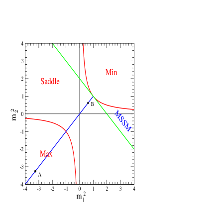
Figure 3: Depending on the values of $m_{1}^{2}$ and $m_{2}^{2}$ the origin of the Higgs potential can be destabilized or not. Absence of UFB directions impose additional constraints on the Higgs masses for the MSSM.

The first condition depends on the quadratic part of the Higgs potential. This is a minimum, a saddle point or a maximum, depending on the mass parameters $m_{i}^{2}$:

$$m_{1}^{2}m_{2}^{2}-|m_{3}^{2}|^{2} > 0\ ,\ m_{1}^{2}+m_{2}^{2}\ >\ 0\ ,\hskip 51.21504pt[\mathrm{Minimum}]$$ (25)

$$m_{1}^{2}m_{2}^{2}-|m_{3}^{2}|^{2} < 0\ ,\hskip 119.50148pt[\mathrm{Saddle\ Point}]$$ (26)

$$m_{1}^{2}m_{2}^{2}-|m_{3}^{2}|^{2} > 0\ ,\ m_{1}^{2}+m_{2}^{2}\ <\ 0\ .\hskip 51.21504pt[\mathrm{Maximum}]$$ (27)

These equations define three regions in the $\{m_{1}^{2},m_{2}^{2}\}$-plane, labelled by ‘Min’, ‘Saddle’ and ‘Max’ in Fig. 1 (where the axes are given in units of $|m_{3}^{2}|$). Such regions are separated by the upper and lower branches of the hyperbola $m_{1}^{2}m_{2}^{2}-|m_{3}^{2}|^{2}=0$. Electroweak breaking can take place in the regions ‘Saddle’ or ‘Max’, while the region ‘Min’ is excluded. The second condition is the absence of UFB directions, along which the quartic part of the potential gets destabilized. In the MSSM the quartic couplings receive only contributions from D-terms, namely $\lambda_{1,2}={1\over 4}(g^{2}+g_{Y}^{2})$, $\lambda_{3}={1\over 4}(g^{2}-g_{Y}^{2})$, $\lambda_{4}=-{1\over 2}g^{2}$, $\lambda_{5,6,7}=0$. Then the potential is indeed stabilized by the quartic terms, except along the D-flat directions $|H_{1}|=|H_{2}|$. It is then required that the quadratic part of $V$ be positive along these directions:

$$m_{1}^{2}+m_{2}^{2}-2|m_{3}^{2}|>0\ .\hskip 56.9055pt[\mathrm{Potential\ bounded\ from\ below}]$$ (28)

This condition applies only to the MSSM and corresponds to the region of Fig. 1 above the straight line tangent to the upper branch of the hyperbola. Since eq. (28) is incompatible with eq. (27), it follows that the MSSM conditions for electroweak breaking are given by eqs.(26,28), as is well known. In Fig. 1 the corresponding region is a subset of the region ‘Saddle’ and is labelled by ‘MSSM’: it is made of the (two) areas between the upper branch of the hyperbola and the tangent line.

In the case that matters to us, when SUSY is broken at a moderately low scale, the $\lambda_{i}$ couplings in (24) also receive sizeable ${\cal O}(F^{2}/M^{4})$ contributions, besides the ${\cal O}(g^{2})$ ones. Therefore condition (28) is no longer mandatory to avoid UFB directions, since the boundedness of the potential can be ensured by imposing appropriate conditions on the $\lambda_{i}$ parameters. Thus the presence of the latter parameters extends the parameter space, relaxes the constraints on the quadratic part of the potential and opens a lot of new possibilities for electroweak breaking. In particular, both alternatives (26, 27) are now possible. This means that most of the $\{m_{1}^{2},m_{2}^{2}\}$ plane can in principle be explored: only the region ‘Min’ is excluded. For instance, now the universal case $m_{1}^{2}=m_{2}^{2}$ is allowed. Actually, in the MSSM these mass parameters could be degenerate at high energy and reach non-degenerate values radiatively by RG running (falling in the region ‘MSSM’ of Fig. 1, typically with $m_{1}^{2}>0$, $m_{2}^{2}<0$). The fact that $m_{2}^{2}$ is the only scalar mass that tends to get negative in this process is considered one of the virtues of the MSSM, in the sense that $SU(2)\times U(1)$ breaking is “natural”. Now, we see that even if the universal condition holds at low-energy we can still break $SU(2)\times U(1)$.

As opposed to the radiative breaking, now electroweak breaking generically occurs already at tree-level. Still, it is “natural” in a sense similar to the MSSM. For example, if all the scalar masses are positive and universal, $SU(2)_{L}\times U(1)_{Y}$ is the only symmetry that can be broken because (with R-parity conserved) the only off-diagonal bilinear coupling among MSSM fields is $m_{3}^{2}\,H_{1}\cdot H_{2}$, which can drive symmetry breaking in the Higgs sector if condition (26) is satisfied. Finally, the fact that quartic couplings are very different from those of the MSSM changes dramatically the Higgs spectrum and properties (which will be tested at colliders, see e.g. [14]). In particular, as will be clear from the example in the next subsection, the MSSM bound on the lightest Higgs field does no longer apply. Likewise, the fact that these couplings can be larger than the MSSM ones reduces the amount of tuning necessary to get the proper Higgs v.e.v.s [6].

4 A simple example.

In this section we present, for illustrative purposes, a simple example (example ”A” of [3]) where many of the previously discussed unconventional features are clear. For simplicity we consider a model that is symmetric under the interchange $H_{1}$ and $H_{2}$, so we can use the general formulae for symmetric potentials of the appendix of [3] to obtain the minimization conditions. Despite this symmetry, the model can accommodate both $\tan\beta=1$ and $\tan\beta\neq 1$ (depending on the choice of parameters). The superpotential, gauge kinetic functions and Kähler potential are chosen as

$$W=\Lambda_{S}^{2}T+\mu H_{1}\cdot H_{2}+{\ell\over 2M}(H_{1}\cdot H_{2})^{2}\ ,\;\;\;\;f_{ab}={\delta_{ab}\over g_{a}^{2}}\left(1+2{\eta_{a}\over M}T\right)\ ,$$ (29)

and

$$K = |T|^{2}+|H_{1}|^{2}+|H_{2}|^{2}$$ (30)

$$- {\alpha_{t}\over 4M^{2}}|T|^{4}+{\alpha_{1}\over M^{2}}|T|^{2}\left(|H_{1}|^{2}+|H_{2}|^{2}\right)+{e_{1}\over 2M^{2}}\left(|H_{1}|^{4}+|H_{2}|^{4}\right)\ ,$$

where all parameters are taken to be real, with $\alpha_{t}>0$. We will sometimes use the auxiliary parameter ${\tilde{m}}=\Lambda_{S}^{2}/M$.

We will analyze the model perturbatively in the Higgs v.e.v.s. We will only retain the first terms of the expansion, which will be sufficient to illustrate the main qualitative features of this example. At zero-th order, i.e. for vanishing Higgs v.e.v.s, we have $\langle T\rangle_{0}=0$, SUSY is broken by $\langle F^{T}\rangle_{0}=-\Lambda_{S}^{2}$, $\tilde{T}$ is the goldstino and the complex $T$ field has mass $m_{T}^{2}=\alpha_{t}\tilde{m}^{2}$. The effects of electroweak breaking start to appear at next order, i.e. when the potential $V(T,H_{1},H_{2})$ is minimized and the Higgses take v.e.v.s. In particular, since $V(T,H_{1},H_{2})$ contains ${\cal O}(TH^{2})$ cubic terms, $T$ receives a small induced v.e.v. $\langle T\rangle=\alpha_{1}\mu v_{1}v_{2}/(\alpha_{t}\Lambda_{S}^{2})$ and $T$-$H$ mass mixing appears. Instead of keeping the field $T$ together with the Higgses, however, we find it more convenient to use the alternative method of decoupling it. We integrate out $T$ and study a reduced effective potential for the Higgs doublets only. This choice is also supported by the special fact that all Higgs boson masses turn out to be ${\cal O}(\lambda v^{2})$ in this model, i.e. naturally lighter than the $T$ mass, which is ${\cal O}({\tilde{m}}^{2})$.

The Higgs v.e.v.s and spectrum are determined by an effective quartic potential $V(H_{1},H_{2})$ with particular values for its mass terms:

$$m_{1}^{2}=m_{2}^{2}=\mu^{2}-\alpha_{1}\tilde{m}^{2}\ ,\;\;\;\;m_{3}^{2}=0\ ,$$ (31)

and quartic couplings

$$\lambda_{1}=\lambda_{2} = {1\over 4}(g^{2}+g_{Y}^{2})+2\alpha_{1}^{2}{\tilde{m}^{2}\over M^{2}}\ ,$$

$$\lambda_{3} = {1\over 4}(g^{2}-g_{Y}^{2})+{2\over M^{2}}(\alpha_{1}^{2}\tilde{m}^{2}-e_{1}\mu^{2})\ ,$$

$$\lambda_{4} = -{1\over 2}g^{2}-2\left(e_{1}+2{\alpha_{1}^{2}\over\alpha_{t}}\right){\mu^{2}\over M^{2}}\ ,$$

$$\lambda_{5} = 0\ ,$$

$$\lambda_{6}=\lambda_{7} = {\ell\mu\over M}\ .$$ (32)

Applying the general formulae given in the appendix of [3] to write down the minimization conditions that give $v^{2}$ and $\sin 2\beta$ in terms of the parameters of the potential we see that concerning the value of $\tan\beta$, we have two possible solutions

$$|\tan\beta|=1\ ,$$ (33)

and

$$\sin 2\beta={\ell\mu/M\over({g^{2}+g_{Y}^{2}})/4+2\hat{e}_{1}\mu^{2}/M^{2}}\ ,$$ (34)

where we use $\hat{e}_{1}\equiv e_{1}+\alpha_{1}^{2}/\alpha_{t}$. Both solutions are possible depending on the choice of parameters, and in both cases ${\rm sgn}(\tan\beta)=-{\rm sgn}(\ell\mu/M)$. It is not restrictive to take $\ell\mu/M<0$, so that $\tan\beta>0$. Using this convention, the explicit expressions for the Higgs masses are the following.

$$\begin{array}[]{ll}\hskip 71.13188pt{\underline{\tan\beta=1}}:&\hskip 71.13188pt{\underline{\tan\beta\neq 1}}:\\ &\\ m_{h}^{2}={\displaystyle 2\left(\alpha_{1}^{2}{\tilde{m}^{2}\over M^{2}}-\hat{e}_{1}{\mu^{2}\over M^{2}}+{\ell\mu\over M}\right)v^{2}}\ ,&m_{h}^{2}={\displaystyle\left[{1\over 4}(g^{2}+g_{Y}^{2})+2\alpha_{1}^{2}{\tilde{m}^{2}\over M^{2}}+{\ell\mu\over M}s_{2\beta}\right]v^{2}}\ ,\vspace{0.2cm}\\ m_{H}^{2}={\displaystyle\left[{1\over 4}(g^{2}+g_{Y}^{2})+2\hat{e}_{1}{\mu^{2}\over M^{2}}-{\ell\mu\over M}\right]v^{2}}\ ,&m_{H}^{2}={\displaystyle-\left[{1\over 4}(g^{2}+g_{Y}^{2})+2\hat{e}_{1}{\mu^{2}\over M^{2}}\right]v^{2}c^{2}_{2\beta}}\ ,\vspace{0.2cm}\\ m_{A}^{2}={\displaystyle-{\ell\mu\over M}v^{2}}\ ,&m_{A}^{2}={\displaystyle-\left[{1\over 4}(g^{2}+g_{Y}^{2})+2\hat{e}_{1}{\mu^{2}\over M^{2}}\right]v^{2}}\ ,\vspace{0.2cm}\\ m_{H^{\pm}}^{2}={\displaystyle\left[{1\over 4}g^{2}+(2\hat{e}_{1}-e_{1}){\mu^{2}\over M^{2}}-{\ell\mu\over M}\right]v^{2}}\ ,&m_{H^{\pm}}^{2}={\displaystyle-\left({1\over 4}g_{Y}^{2}+e_{1}{\mu^{2}\over M^{2}}\right)v^{2}}\ .\end{array}$$ (35)

Notice that acceptable solutions with $\tan\beta=1$ can be obtained even if we set $e_{1}=0$, which further simplifies the model. To obtain solutions with $\tan\beta\neq 1$, however, we need $e_{1}<0$. Also notice that, in the phase with $\tan\beta\neq 1$, the value of $\tan\beta$ is only determined up to an inversion ($\tan\beta\leftrightarrow 1/\tan\beta$), which in fact leaves the spectrum invariant. This is a consequence of the original discrete symmetry, and we can conventionally take $\tan\beta\geq 1$.

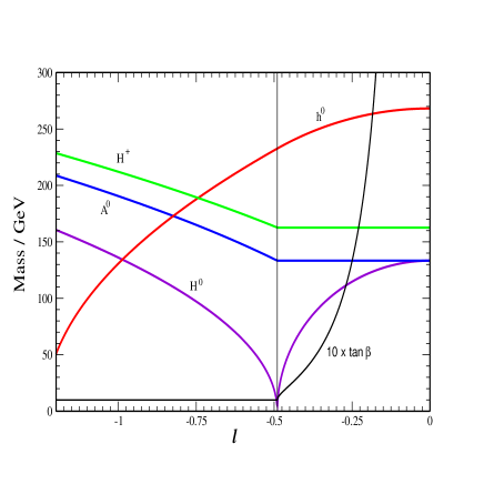
Figure 4: Higgs spectrum as a function of the superpotential parameter $\ell$. Also shown is $\tan\beta$ (scaled by a factor 10).

In Fig. 4 we show a numerical example where both phases of the model are visible. We have fixed $\mu/M=0.6$, $e_{1}=-1.3$, $\tilde{m}/M=0.5$, $\alpha_{t}=3.0$, $\alpha_{1}\simeq\mu^{2}/\tilde{m}^{2}+\epsilon^{2}$ (with $0<\epsilon^{2}\ll 1$) and vary $\ell$. For each parameter choice, the overall mass scale $M$ is adjusted so as to get the right value of $v=246$ GeV. The closer $\alpha_{1}$ is to $\mu^{2}/\tilde{m}^{2}$ the larger $M/v$ can be. The figure shows the Higgs spectrum and the parameter $\tan\beta$ (scaled by a factor 10 for clarity) as a function of the coupling $\ell$. For $\ell\leq\ell_{0}$, with

$$\ell_{0}\equiv{M\over\mu}\left[{1\over 4}(g^{2}+g_{Y}^{2})+2\hat{e}_{1}{\mu^{2}\over M^{2}}\right]\ ,$$ (36)

the minimum lies at $\tan\beta=1$, while for $\ell>\ell_{0}$, $\tan\beta$ increases with $\ell$. For the choice of parameters used in this figure, $\ell_{0}\simeq-0.49$. The spectrum is continuous across the critical value $\ell_{0}$, although the mass of the ‘transverse’ Higgs, $H^{0}$, goes through zero, as was to be expected on general grounds for symmetric potentials. We see that, except in the neighborhood of $\ell_{0}\simeq-0.49$ or for too negative values of $\ell$, the Higgs masses are sufficiently large to escape all current experimental bounds (which are also lower than usual due to singlet admixture, although this is typically a small effect). There is even a region of parameters for which $h^{0}$ is the heavier of the Higgses, beyond the usual limit of $m_{h^{0}}\ln{m_{t}^{2}\over Q^{2}}200$ GeV [15] that applies in generic SUSY models only when they are perturbative up to the GUT scale.

5 Conclusions

When the scales of SUSY ($\sqrt{F}$) and SUSY mediation ($M$) are close to the electroweak scale, the usual MSSM, where the effects of SUSY breaking in the observable sector are encoded in a set of soft SUSY-breaking terms of size ${\cal O}(F/M)$, may not give an accurate enough description of electroweak scale physics. Additional effects can be relevant, in particular non-negligible contributions to hard breaking terms, such as ${\cal O}(F^{2}/M^{4})$ contributions to quartic Higgs couplings. In fact, the latter contributions can compete with (and may take over) the usual ($D$-term induced) MSSM quartic Higgs couplings, giving rise to a quite unconventional Higgs sector phenomenology.

In this brief review of the phenomenology of these models we have focussed on the Higgs sector, and we have analyzed, following [3], the interplay of SUSY and electroweak breaking. We have seen how the Higgs potential resembles that of a 2HDM, where the quadratic and quartic couplings can be traced back to the original couplings in the effective superpotential and Kähler potential. The goldstino supermultiplet can have non-negligible interactions with the Higgs fields, and its scalar component can also mix with them as a result of electroweak breaking.

The presence of extra quartic couplings that may be larger than the usual ones opens novel opportunities for electroweak breaking. The breaking process is effectively triggered at tree-level and presents important differences with the usual radiative mechanism. Electroweak breaking can occur in a much wider region of parameter space, i.e. for values of the low-energy mass parameters that are normally forbidden. A further advantage of the extra quartic couplings is that their presence reduces the amount of tuning necessary to get the correct Higgs v.e.v.s. These new quartic couplings also imply that the spectrum of the Higgs sector is dramatically changed, and the usual MSSM mass relations are easily violated. In particular, the new quartic couplings allow the lightest Higgs field to be much heavier ($\lower 3.01385pt\hbox{$\;\stackrel{{\scriptstyle\textstyle<}}{{\sim}}\;$}500$ GeV) than in usual supersymmetric scenarios.

We have illustrated these facts by means of an example, in which we have analyzed the Higgs potential and the electroweak breaking process, making clear the unconventional features that emerge.

References

- [1] H. E. Haber and G. L. Kane, Phys. Rept. 117 (1985) 75; H. P. Nilles, Phys. Rept. 110 (1984) 1; N. Polonsky, Lect. Notes Phys. M68 (2001) 1 [arXiv:hep-ph/0108236].
- [2] N. Polonsky and S. Su, Phys. Lett. B 508, 103 (2001) [arXiv:hep-ph/0010113]; N. Polonsky, Nucl. Phys. Proc. Suppl. 101, 357 (2001) [arXiv:hep-ph/0102196].
- [3] A. Brignole, J. A. Casas, J. R. Espinosa and I. Navarro, Nucl. Phys. B (in press) [arXiv:hep-ph/0301121].
- [4] A. Brignole, Nucl. Phys. B 579 (2000) 101 [arXiv:hep-th/0001121].
- [5] J. Bagger and E. Poppitz, Phys. Rev. Lett. 71 (1993) 2380 [arXiv:hep-ph/9307317]; J. Bagger, E. Poppitz and L. Randall, Nucl. Phys. B 455 (1995) 59 [arXiv:hep-ph/9505244].
- [6] J. A. Casas, J. R. Espinosa and I. Hidalgo, to appear.
- [7] D. A. Dicus, S. Nandi and J. Woodside, Phys. Rev. D 41 (1990) 2347; A. Brignole, F. Feruglio and F. Zwirner, Nucl. Phys. B 501 (1997) 332 [arXiv:hep-ph/9703286], JHEP 9711 (1997) 001 [arXiv:hep-th/9709111], A. Brignole, F. Feruglio and F. Zwirner, Nucl. Phys. B 516 (1998) 13 [Erratum-ibid. B 555 (1999) 653] [arXiv:hep-ph/9711516]; A. Brignole, F. Feruglio, M. L. Mangano and F. Zwirner, Nucl. Phys. B 526 (1998) 136 [Erratum-ibid. B 582 (2000) 759] [arXiv:hep-ph/9801329].
- [8] A. Brignole, F. Feruglio and F. Zwirner, Phys. Lett. B 438 (1998) 89 [arXiv:hep-ph/9805282]; A. Brignole, E. Perazzi and F. Zwirner, JHEP 9909, 002 (1999) [arXiv:hep-ph/9904367]; F. Mori and A. A. Natale, Mod. Phys. Lett. A 15 (2000) 1099.
- [9] J. A. Casas, J. R. Espinosa and I. Navarro, Nucl. Phys. B 620 (2002) 195 [arXiv:hep-ph/0109127].
- [10] J. Wess and J. Bagger, Princeton, USA: Univ. Pr. (1992) 259 p.
- [11] P. Fayet, Phys. Lett. B 70 (1977) 461; R. Casalbuoni, S. De Curtis, D. Dominici, F. Feruglio and R. Gatto, Phys. Lett. B 215 (1988) 313, Phys. Rev. D 39 (1989) 2281.
- [12] L. J. Hall, J. Lykken and S. Weinberg, Phys. Rev. D 27 (1983) 2359; S. K. Soni and H. A. Weldon, Phys. Lett. B 126 (1983) 215; G. F. Giudice and A. Masiero, Phys. Lett. B 206 (1988) 480; V. S. Kaplunovsky and J. Louis, Phys. Lett. B 306 (1993) 269 [hep-th/9303040]; A. Brignole, L. E. Ibanez and C. Munoz [hep-ph/9707209].
- [13] F. Boudjema and A. Semenov, Phys. Rev. D 66 (2002) 095007 [arXiv:hep-ph/0201219]; J. F. Gunion and H. E. Haber, Phys. Rev. D 67 (2003) 075019 [arXiv:hep-ph/0207010].
- [14] M. Carena and H. E. Haber, Prog. Part. Nucl. Phys. 50 (2003) 63 [arXiv:hep-ph/0208209].
- [15] J. R. Espinosa and M. Quiros, Phys. Rev. Lett. 81 (1998) 516 [hep-ph/9804235].