IF - 1576/2003
IFT-P.033/2003
Discriminating among Earth composition models using geo-antineutrinos
Abstract
It has been estimated that the entire Earth generates heat corresponding to about 40 TW (equivalent to 10,000 nuclear power plants) which is considered to originate mainly from the radioactive decay of elements like U, Th and K, deposited in the crust and mantle of the Earth. Radioactivity of these elements produce not only heat but also antineutrinos (called geo-antineutrinos) which can be observed by terrestrial detectors. We investigate the possibility of discriminating among Earth composition models predicting different total radiogenic heat generation, by observing such geo-antineutrinos at Kamioka and Gran Sasso, assuming KamLAND and Borexino (type) detectors, respectively, at these places. By simulating the future geo-antineutrino data as well as reactor antineutrino background contributions, we try to establish to which extent we can discriminate among Earth composition models for given exposures (in units of kt yr) at these two sites on our planet. We use also information on neutrino mixing parameters coming from solar neutrino data as well as KamLAND reactor antineutrino data, in order to estimate the number of geo-antineutrino induced events.
pacs:
13.15.+g,14.60.Lm,95.55.Vj,95.85.RyI Introduction
There is much about the Earth’s heat engine that is unknown. The main datum is the surface heat flow, as most of the Earth is hidden from view. The total heat flux is presently estimated to be about 40 TW, which, however, suffers from uncertainties due to the size of its local variations and inaccessibility of much of Earth’s surface.
We know that there are radioactive isotopes in the Earth that can produce heat through decay. Although the rate of heat generation by decay of unstable radioactive nuclides is tiny, if it is integrated over the entire volume of the Earth, the total heat flux becomes huge. Radiogenic heat, evidently, must be an important source of internal heat production. However, questions as how much of the Earth’s heat generation is from radiogenic origin, how much from residual heat remaining from the formation of the Earth or from the release of gravitational energy as the Earth contracts, have not yet been answered in a satisfactory way.
In the context of modeling the thermal state and thermal history of the Earth it is important to know the specific heat production of the chief heat-producing radionuclides such as 40K, 238U, 232Th and 87Rb, encountered on surface layers and supposed to exist also in interior layers. The heat that drives mechanical motion in the mantle presumably comes mostly from radioactivity. In the radioactive decay process, a portion of the mass of each decaying nuclide is converted to energy. Most of this is the kinetic energy of emitted and particles or of rays, which is fully absorbed by rocks within the Earth and converted to heat.
For decays, however, part of the energy is carried away by emitted neutrinos and antineutrinos. Clearly, measuring the neutrino and antineutrino fluxes from the Earth can provide a unique way to access information on the internal structure and dynamics of our planet Eder ; Avilez ; Krauss ; Kobayashi ; Chen ; Ragh ; fiorentini1 ; fiorentini2 ; fiorentini3 .
This can be done, at least for electron-antineutrinos () coming from 238U and 232Th decays, the former producing 6 and the latter 4 per decay chain within the energy reach of current and near future neutrino detectors. Antineutrinos from these elements have higher energies than those that come from 40K and 87Rb, and are detectable at liquid scintillator detectors such as KamLAND kamland and/or Borexino borexino through the inverse -decay reaction, where the detection threshold energy is MeV.
Different Earth composition models predict different total amount of U and Th in the mantle, which lead to different total heat flux from radiogenic origin. Moreover, the fact that concentration of such elements is much larger (a factor of times) in the continental crust (with typical thickness km) than the oceanic one (with typical thickness km) and continents and ocean are not uniformly distributed over the Earth make the geo-antineutrino flux different from place to place.
Quite recently, in Ref. fiorentini1 , geo-antineutrino fluxes from various Earth composition models have been estimated (before the first KamLAND results were reported) and then in Ref. fiorentini2 , the first KamLAND data, which contained possible geo-antineutrino candidate events kamland , have been analyzed, and it was concluded that practically all Earth composition models are consistent with the current data. Moreover, the accumulated data so far at KamLAND is not enough to establish the presence of geo-antineutrinos kamland and we must wait for future data.
In this work, we will try to go beyond the above mentioned papers, by investigating to which extent liquid scintillator (type) detectors such as KamLAND and/or Borexino can be used to help in discriminating among different geophysical models of heat production by measuring antineutrinos in the energy range produced inside the Earth. We show how much one can improve the quantitative understanding of the radiogenic contribution to terrestrial heat in about a decade of operation.
II Earth As a Antineutrino Source
Antineutrinos are produced inside the Earth in radioactive decays mainly of 40K, 238U, 232Th and 87 Rb. These elements are classified as lithophile elements in geophysics and considered to be accumulated more in the Earth’s crust. The abundance of these isotopes, although of prime geophysical importance, is only known at or near the surface of the Earth. Among these geo-antineutrinos, the one come from 238U and 232Th have higher energies. The maximal neutrino energy from the former and the latter are, respectively, = 3.26 MeV and = 2.25 MeV, which are above the threshold of existing anti-neutrino detector such as KamLAND kamland and Borexino borexino .
Here we consider, as our references, four different models which predict the distributions of 238U and 232Th in the Earth. We do not consider neutrinos coming from 40K and 87Rb because energies of these neutrinos are below the threshold of detectors we consider in this work. For all models, we have considered three regions, namely, continental crust, oceanic crust and mantle, with different average concentrations of U and Th. We ignore any contribution from the core. The distribution of radioactive elements are supposed to be uniform within each region. Although the concentrations of these radioactive elements are considered to be much smaller in the mantle than in the crust, the total geo-antineutrino flux from the whole mantle can be comparable to that coming from the crust because of the much larger volume.
Since the total mass of U in the crust is estimated to be kg, and Si represents about 15% of the Earth mass, kg, the other masses in the crust and in the mantle can be obtained for each model from the mass ratios they provide. In this paper we will fix in the crust to the above estimated value, but we should point out that this number is known with 50% uncertainty. The average concentration of U in the continental crust is estimated to be 1.7 ppm wedepohl whereas that in the oceanic one is estimated to be 0.1 ppm taylor . We will assume here these numbers as reference values but as we will discuss later it is important to know the local variations of concentration as well as as the of the crustal thickness at each experimental site.
The models can be thus classified by the amount of U they predict for the mantle . In this work, we follow the classification of models considered in Ref. fiorentini1 ; Ragh , whose characteristic will be described below.
II.1 Chondritic Earth Model
The Chondritic Earth model assumes for the Earth’s gross composition that of the oldest meteorites, the carbonaceous chondrites. The mass ratios for these meteorites And are: , and Bro . Radiogenic production in the chondritic model easily accounts for 75% of the observed heat flow, about 30 TW. U and Th provide comparable contributions, each a factor of two below that of K. In this model, by taking into account that the total mass of the mantle is 4.1 kg (68 % of the total Earth mass), concentration of U in the mantle is about 0.006 ppm.
II.2 Bulk Silicate Earth (BSE) Model
The Bulk Silicate Earth (BSE) model provides a description of geological evidence coherent with geochemical information. It describes the primordial mantle, prior to crust separation. The mass ratios here are: , and . In this BSE model the present radiogenic production, mainly from U and Th, accounts for about one half of the total heat flow, 20 TW. The antineutrino luminosities from U and Th are rescaled by a factor 1.3 whereas K, although reduced by a factor of 5, is still the principal antineutrino source. Concentration of U in the mantle is 0.01 ppm Mc .
II.3 Fully Radiogenic (FR I) Model
One can conceive a model where heat production is fully radiogenic, with fixed at the terrestrial value and at the chondritic value, which seems consistent with terrestrial observations fiorentini1 . All the abundances are rescaled so as to provide the full heat flow. All particle production rates are correspondingly rescaled by a factor of two with respect to the predictions of the BSE model. The concentration of U in the mantle for this model is about 0.03 ppm.
II.4 Modified Fully Radiogenic (FR II) Model
This model is similar to the previous one, the abundances of U and Th are also rescaled with respect to BSE but it assumes that as an extreme case, the total heat flow of 40 TW are produced in the Earth only by U and Th, completely ignoring K, as considered in Ref. Ragh . This is an extreme, geo-antineutrino fluxes much larger than this limit would need serious alteration of source distribution. The concentration of U in the mantle for this model is about 0.04 ppm.
III Analysis Method
Here we explain how we calculate the expected number of geo-antineutrino events, for each one of the four models presented in the previous section, at a certain detector position for a given exposure. To try to distinguish models we have used a function minimization which is explained at the end of this section.
III.1 Calculation of the antineutrino fluxes from Th and U decay chains
We would like to calculate the flux of antineutrino produced in the Earth by the decay of a certain isotope that reach a detector for all four geophysical composition models presented in the previous section. Following Refs. fiorentini1 ; fiorentini2 , differential flux of antineutrinos produced in the decay chain of radioactive isotope that will be measured at a detector position on the Earth, can be expressed by the following integral performed over the Earth volume ,
| (1) |
where is the matter density, , , and are, respectively, the concentration, life time, atomic mass and the number of antineutrinos emitted per decay chain corresponding to element . is the normalized spectral function for element spectrum , is the survival probability, which can be averaged out, as a good approximation, and bring out from the integral the term:
| (2) |
where is the mixing angle responsible for the solar neutrino problem, which is fixed to the current best fitted value, , obtained by combining the solar neutrino and KamLAND data NTZ03 , except in Sec. IV.2 where is treated as a free parameter to be fitted. We note that the Earth matter effect on geo-antineutrino oscillation is very small and therefore, can be safely neglected in our analysis.
The integration in Eq. (1) can be approximately divided into three distinct contributions, from continental crust (cc), oceanic crust (oc) and mantle (m), assuming that the matter density and the concentration of , are approximately constant within these three regions and ignoring any contribution from the core, as assumed in Ref. fiorentini1 , as follows,
| (3) |
where km is the radius of the Earth, and we have defined the neutrino luminosity, , and a factor which depend on the crust thickness distribution over the Earth as well as the detector location, ( cc, co, m), as
| (4) | |||||
| (5) |
where , and are, respectively, the volume, the average concentration of U or Th and matter density of region . We can also write the observable luminosities , in units of particles per second, for masses in units of kg, as
| (6) |
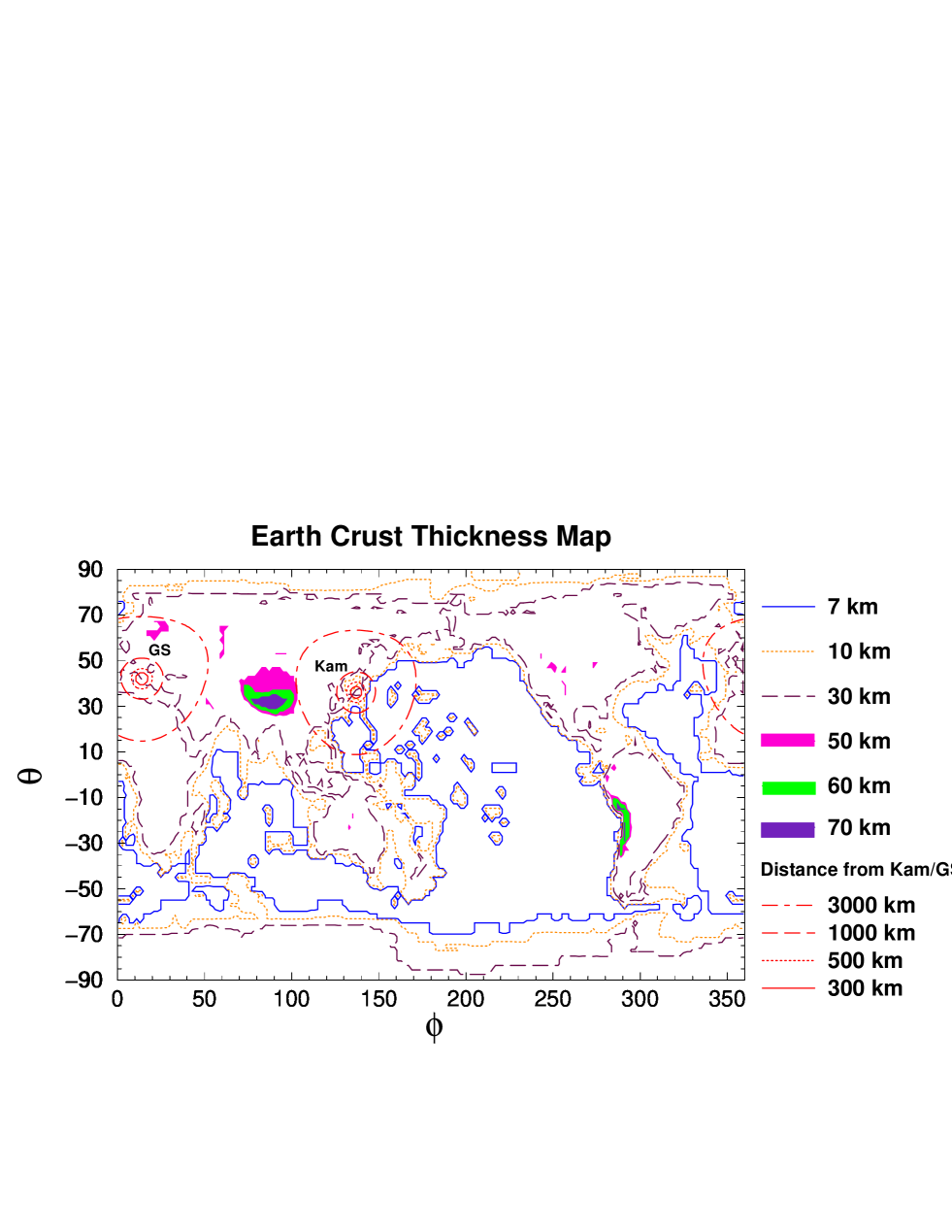
In Eq. (5), indicates the thickness of the shell (mantle or crust) at the position . For the mantle we have simply used , giving . For the crust calculation (typical thickness being 35 km for continental crust and 7 km for oceanic one), we have used the Earth Crust Thickness map ThicknessMap , which was obtained based on seismology, to compute the at a given detector position. Earth’s crust is divided into 16200 cells of where within each cell, the crust thickness is assumed to be constant. See Fig. 1 for a schematic illustration of the cell. In Fig. 2 we show some iso-contours of Earth crust thickness in the plane (corresponding to longitude and latitude) based on this crustal map model ThicknessMap which we will use in this work.
We observe that in our model assumption the predicted ratio of the geo-antineutrino fluxes from U and Th does not depend on details of the integration in Eq. (1) but is given by the following simple formula for any model we consider,
| (7) |
Note that we are assuming uniform U/Th distribution so that the ratio of the total amount of Th and U, , is considered to be 3.8 in any of the input models under investigation.
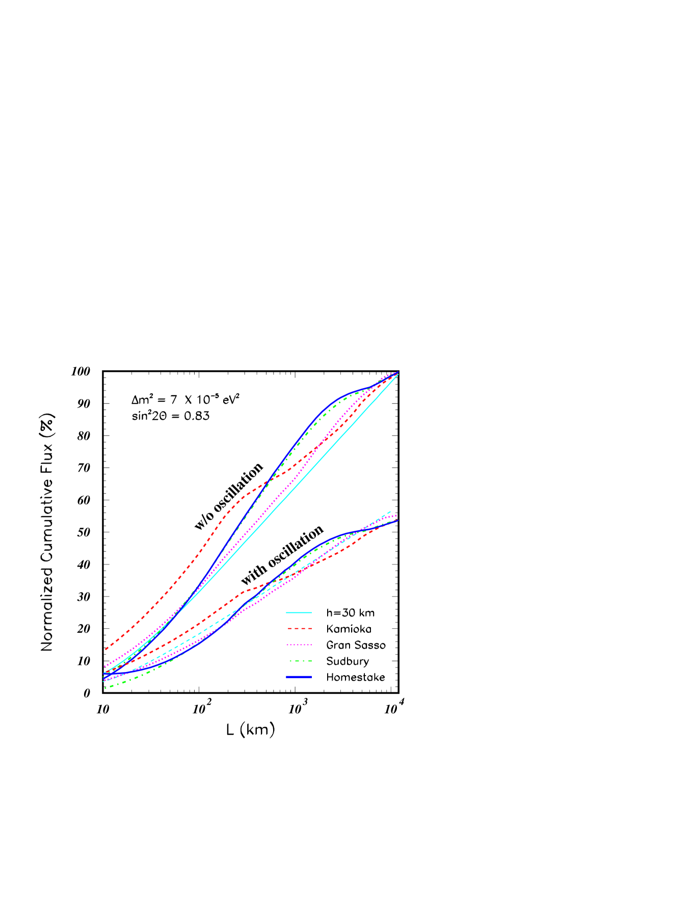
We have thus the basic equations for determining radiogenic heat production and neutrino flows from models of the Earth composition. In order to have some feeling about the local variation of geo-antineutrino fluxes due to the variable crustal thickness, in Fig. 3, we present the normalized cumulative geo-antineutrino flux coming from the continental as well as oceanic crust (without contributions from the mantle) at Kamioka, Gran Sasso, Homestake and Sudbury, as a function of the distance () from the source to the detector, computed using the information from the Earth Crust thickness map ThicknessMap . We note that due to the fact that the abundance of U/Th is much larger in the continental crust than in the oceanic one, the geo-antineutrino flux from the former is dominant.
Since the typical size of the crustal cell at these detector sites is of the order of 100 km, we can only reliably compute for distances equal or larger than this distance. In Fig. 3 we have extrapolated each curve down to 10 km, as a first approximation. For the sake of comparison, we have also plotted the hypothetical case where the entire Earth crust has a uniform thickness of 30 km. Neutrino oscillations were not taken into account in the calculation of the upper five curves but were included in the lower five. These latter curves have been normalized with respect to the no oscillation case.
From this plot, as far as the geo-antineutrino flux coming from the Earth crust is concerned, we can see that about 30-40 % of the total crustal antineutrino flux comes from a distance within 100 km and about 50-60 % from a distance within 500 km from the detector. We note that this flux is about 80%, 65%, 40% and 33% of the total flux, respectively, for Chondritic, BSE, FR I and FR II models. This implies that it is very important to know rather well, with better than resolution, the variation of the crustal thickness near the detector as well as the local variation of the concentration of radioactive elements.
III.2 Number of geo-antineutrino events
The number of geo-antineutrino induced events from the decay chain of element in the -th energy bin, , is:
| (8) |
where is the number of free protons in the fiducial volume of the detector, is the exposure time, is the detection efficiency, which is assumed to be 100 % for simplicity. This integral, which is easily computed using the cross section given in Ref. cross , is understood to be performed in a certain energy bin.
We divide the number of events in the positron prompt energy range 0.9-2.6 MeV into 4 bins with an interval of 0.42 MeV following Ref. kamland . Note that the prompt energy is related to neutrino energy as where and are respectively, mass of neutron, proton and electron. The number of events in th bin is defined as the sum of events coming from U and Th, . We note that the 1st two lower energy bins contains events coming from both U and Th induced geo-antineutrinos whereas the last two higher energy bins contain only events coming from Th.
III.3 minimization
We define the function for our geo-antineutrino analysis as follows,
| (9) |
where , and are respectively, the number of (simulated) observable events (geo + reactor antineutrinos), the number of theoretically expected events coming from geo-antineutrinos and from nuclear reactors in the neighborhood of the detector. As mentioned before, geo-antineutrinos will only contribute to the first four bins. We have taken into account in our calculation the total statistical error as well as a 6% systematic error only for reactor antineutrino events kamland . Since currently no detector has enough data in the energy region interesting for geo-antineutrino observations, we simulate according to the Earth composition models, taking into account the reactor antineutrino background for a given exposure and site. Here, for simplicity, we ignore the systematic error for geo-antineutrinos as it is expected to be not so important compared to the statistical one for the exposure we consider in this work.
The above will be minimized with respect to: (i) and , the total geo-antineutrino flux coming from Th and U at a given detector site; (ii) assuming Th/U ratio fixed; (iii) and , assuming Th/U ratio fixed. In the first two cases the neutrino mixing parameters are fixed to their best fitted values, in the latter only is fixed (see the discussion in the following sections for further details). In addition, for some of our analyses, we have also added the function for solar neutrinos, , which was obtained in Ref. NTZ03 .
IV Results
IV.1 Determination of Geo-antineutrino fluxes
We first discuss the determination of geo-antineutrino fluxes at Kamioka as well as Gran Sasso sites where the former (latter) has larger (significantly smaller) reactor antineutrino background. In this work, we have assumed the reactor antineutrino flux at Gran Sasso 5 times smaller than at Kamioka site, however, it can actually be even smaller Ragh . In this subsection, we assume that solar neutrino mixing parameter will be determined with a good precision in the future. See, for instance, Ref. sol_param for a discussion on the perspectives of future determination of the solar neutrino mixing parameters. Due to the effect of oscillation, the observable flux suffers a reduction of , which implies that the original flux must be understood as 1.7 times larger than we assumed at the detector site.
Strictly speaking, experiments can only measure the total flux of geo-antineutrinos for a certain energy range, regardless of their origin (mantle, crust). They cannot directly access the amount of U and/or Th in the crust and mantle separately. Therefore, to be more conservative, we first try to consider the total geo-antineutrino fluxes from U and Th as free parameters to be fitted by the data for a given input model assumption. Since we still do not have enough data in the geo-antineutrino energy range ( MeV), currently KamLAND has reported data only for about 0.16 ktyr exposure kamland , we have simulated future data according to each one of the Earth composition models. We have used these simulated data points as an input in our analysis. By performing a analysis we have investigated if the experiments can correctly reproduce the input data and distinguish among different models.
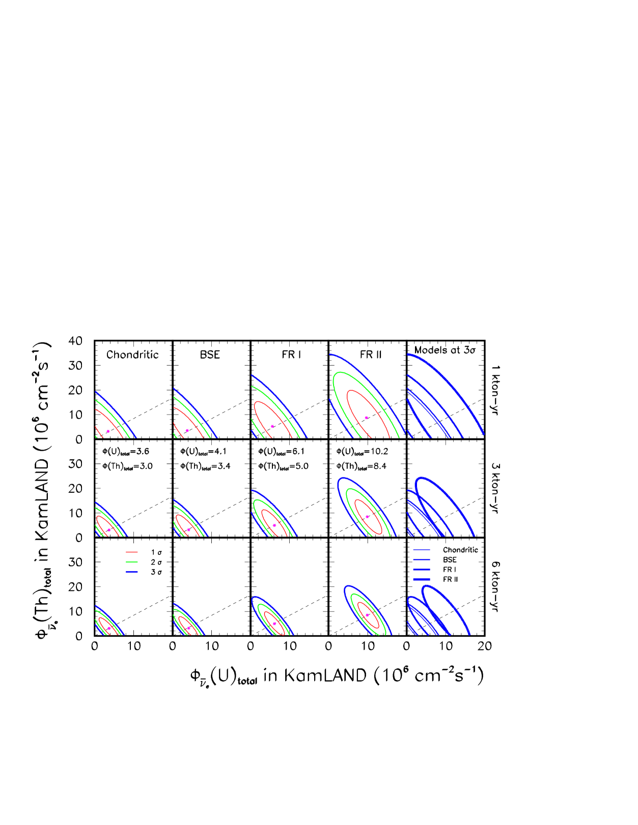
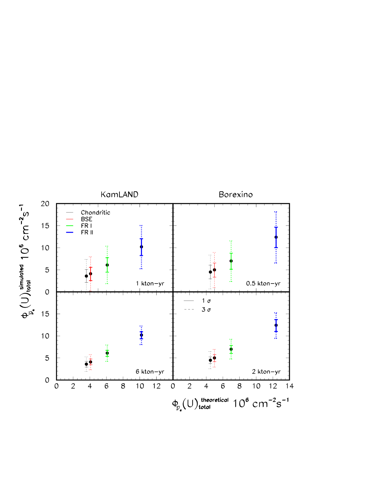
First we have estimated the required exposure, in units of ktyr to identify the presence of geo-antineutrino flux for an assumed model input, leaving the two components of the geo-antineutrino flux, coming from U and Th, completely free in our fit. The results are shown in Table I. The numbers in the table are the detector exposure, at each site, required to rule out or accept each model at 3 level. The actual fiducial volume of KamLAND (Borexino) is about 0.4 (0.1) kt, which means one has to multiply by a factor 2.5 (10) the number found in Table I in order to translate it to the actual detector exposure time. As naturally expected, the larger the input flux, the easier to identify the model, and therefore we need a smaller exposure to rule it out. If, for instance, a detector such as KamLAND, does not see geo-antineutrinos at the 3 level after 0.46 ktyr exposure, it can rule out the FR II model, but at this point it cannot say anything about the other models. On the other hand, if KamLAND measures geo-antineutrinos at this exposure, then FR II has to be interpreted as the preferred model, and so forth.
| Chondritic | BSE | FR I | FR II | |
|---|---|---|---|---|
| Site | ||||
| Kamioka | 1.7 | 1.3 | 0.67 | 0.46 |
| Gran Sasso | 0.89 | 0.71 | 0.38 | 0.26 |
In Fig. 4, we present in the plane, to which extent we can determine geo-antineutrino fluxes in the presence of neutrino oscillations for given input model fluxes and exposure (in units of ktyr) at the Kamioka site. In all cases we are able to correctly reproduce the input fluxes as the best fit points (indicated by stars) in our fit, which, however, does not necessarily mean we can distinguish models with enough significance (see the text below). Unfortunately it seems to be extremely difficult to distinguish between BSE and Chondritic models, independently of the detector exposure we have considered here. From this plot, we can conclude that for 1 ktyr of exposure, it is not possible to distinguish among the four models considered. However, after 3 ktyr of exposure, one start to have some sensitivity to distinguish models, namely, Chondritic/BSE from FR II. After the maximal exposure considered, 6 ktyr of data, one can almost always distinguish FR II from any of the other models. It is worthwhile to note that even for the maximal exposure and maximal flux (FR II) considered here, it is not possible to exclude a null Th induced geo-antineutrino flux, whereas it is sometimes possible to exclude a null U induced one.
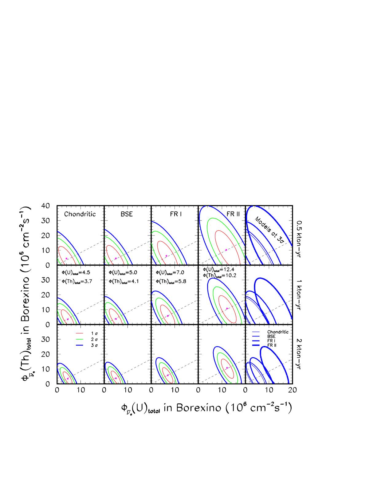
In Fig. 5, we present the same plot but for the Gran Sasso site, assuming a significantly less reactor neutrino background, 5 times smaller than at the Kamioka site. In this case, one can achieve the same sensitivity for the flux determination with much less exposure compared to the Kamioka site. Roughly speaking, ktyr exposure at Gran Sasso correspond to ktyr at Kamioka, which we can see by comparing Figs. 4 and 5. The general behavior of the allowed regions are very similar to that for Kamioka site apart from this difference.
In Fig. 6, we show with which precision the total U induced antineutrino flux can be determined by the experiments, further imposing that the ratio between the total U and Th mass in the Earth is fixed to be constant, , in the fit. Note that this reasonable assumption, based on meteorite and Earth surface data, is not very important in distinguishing models but allows for a better precision in flux determination. In this case, we have only one free parameter, , to be fitted. In 6 ktyr at Kamioka, the total U flux can be determined within less than 10 % uncertainty, independently of the model. The precision it can be determined at Gran Sasso, after 2 ktyr exposure, is a bit over 10 %.
Let us now translate the flux uncertainties we have estimated into heat uncertainties, in order to compare our results with those of Ref. fiorentini3 . As one can easily understand from Eq. (8) of that paper, we can write the total heat, , as a function of the geo-antineutrino flux as
| (10) |
where and are positive constants satisfying . This implies that the relative heat uncertainty is always greater than the relative flux uncertainty, that is,
| (11) |
We have roughly estimated that the flux uncertainties of the order of 10 %, that can be achieved at Kamioka with 6 ktyr exposure, correspond to 15-30% in heat uncertainties, consistent with the results presented in Ref. fiorentini3 .
IV.2 Dependence on the solar mixing angle
So far, we have fixed the solar mixing angle to its current best fitted value. How our ignorance about the precise value of the solar mixing angle can aggravate our results? To answer this question, we perform a fit leaving as a free parameter. For this purpose we will combine present solar neutrino data with future simulated reactor and geo-antineutrino data.
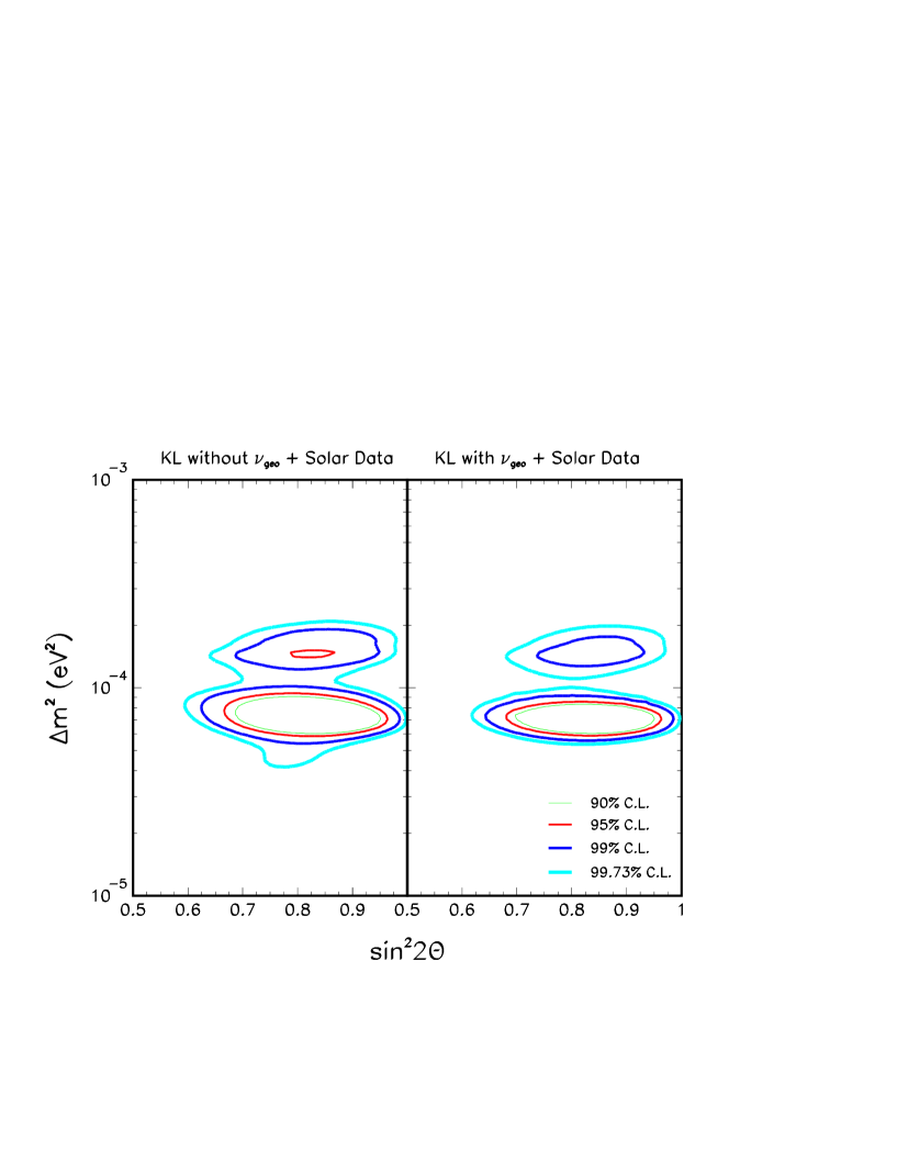
As a first step, to see how the observation of geo-antineutrinos can affect the determination of the mixing angle, we have analyzed the present KamLAND reactor antineutrino data (17 bins) allowing for geo-antineutrino contributions in the first 4 bins, as performed by the authors of Ref. fiorentini2 leaving Th and U antineutrino fluxes free but imposing that the ratio between the total U and Th mass in the Earth is fixed to be constant, , as in the end of the previous section. In Fig. 7, we show the result we have obtained. In agreement with the result in Ref. fiorentini2 , the allowed region becomes somewhat smaller when we include events which can be interpreted as geo-antineutrinos. However, we have confirmed that if U and Th contributions were treated as independent free parameters, the allowed region would not shrink as much, as recently pointed out by Inoue in Ref. kamland . Some events observed in the energy range MeV can be attributed to geo-antineutrinos, but the claim that geo-antineutrinos have been observed can not be made at this point due to small statistics (see discussion in previous section).
We further proceed, by combining the KamLAND data with the current solar neutrino one. The final result is shown in the right panel of Fig. 8, where we have also presented the result without the geo-antineutrino constraint in the left panel taken from Ref. NTZ03 . The allowed region becomes somewhat smaller but essentially has not changed. This is quite understandable as solar neutrino data are dominating in the determination of the mixing angle at this point.
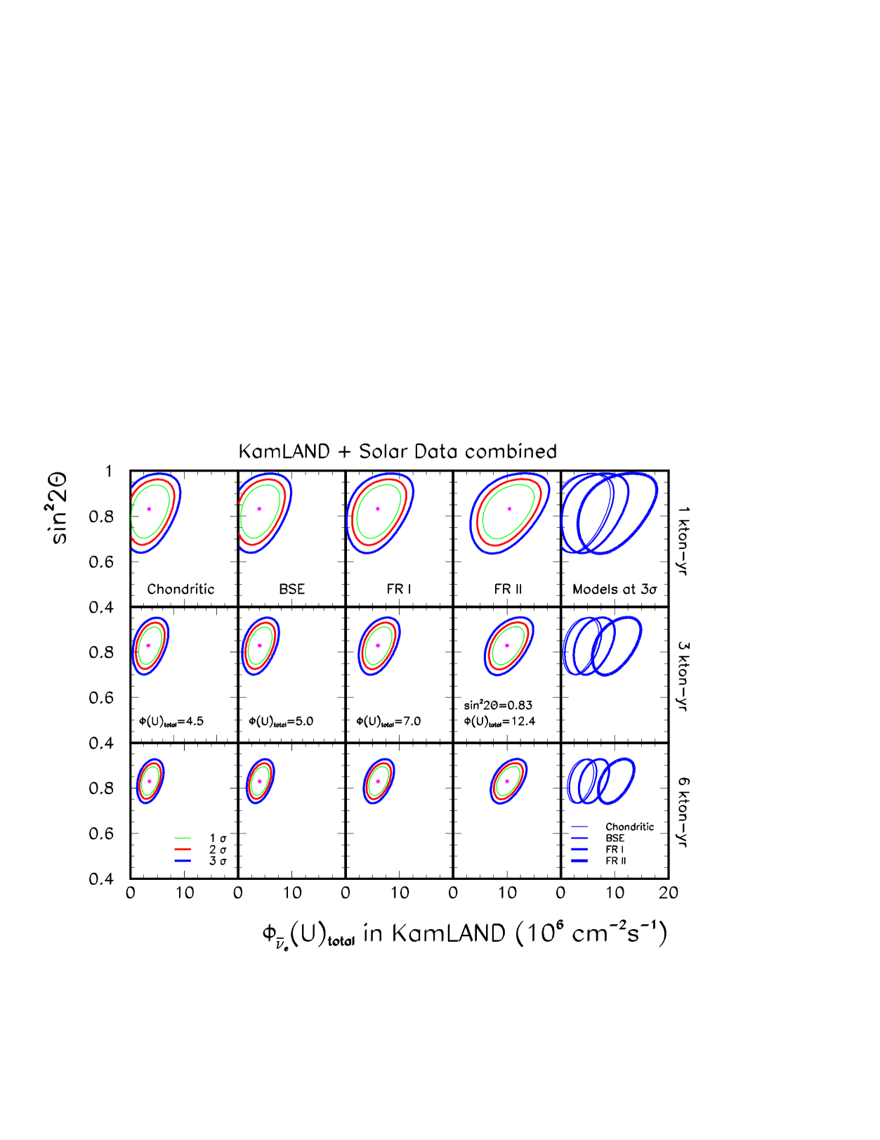
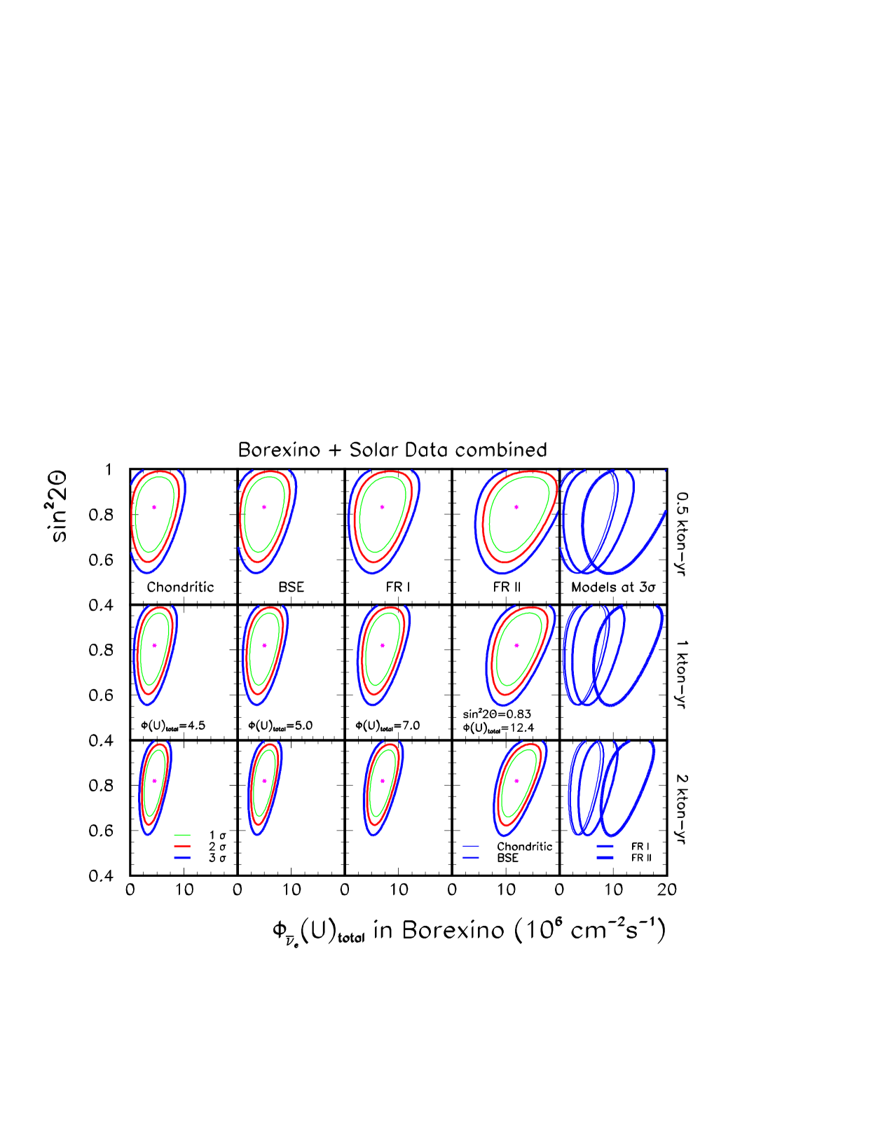
Finally, we combine the simulated future reactor and geo-antineutrino data with the present solar neutrino data. In order to see how the discrimination power of composition models depends on our ignorance of the precise value of the solar mixing angle, for a given input value (fixed to be the current best fit value) as well as (U), we perform a fit leaving (U) and as free parameters. In this fit, we assume the ratio between the total U and Th mass in the Earth to be constant, , for simplicity. This is quite reasonable for our purposes here as the discrimination power among models does not seem to depend very much on this assumption, as we have discussed in the previous subsection.
In Figs. 9 and 10 we plot the allowed region for (U) and for the Kamioka and Gran Sasso sites. The reduction of the allowed range of from 1 to 6 ktyr exposure is essentially due to reactor antineutrinos. We observe that our ignorance on the exact value of does not influence very much the determination of (U), so our conclusions in the previous subsection do not essentially change.
V Discussion and Conclusion
The amount of radioactive elements in the Earth is not well known. The total quantity of U and Th in the Earth, however, can be directly measured by neutrino detectors. Presently KamLAND data imply that the Earth radiogenic heat output can be anything between 0 and 110 TW kamland and all Earth composition models are compatible fiorentini2 . We have studied how this can be improved by future data.
We have investigated to which extent U and Th geo-antineutrino fluxes can be determined by neutrino detectors in a decade of exposure. We have considered KamLAND at Kamioka and Borexino at Gran Sasso as our reference detectors and sites. We have found, as we showed in Table I, that within a few years with a relatively small amount of exposure, it is possible to establish the presence of geo-antineutrinos unless their flux is significantly smaller than expected. However, to discriminate among different Earth composition models, considerably longer exposure is required. We found that in 6 ktyr at Kamioka, the total U flux can be determined within less than 10 % uncertainty, independently of the model we considered. The precision it can be determined at Gran Sasso, after 2 ktyr exposure, is slightly larger than 10 %. We note that at Gran Sasso the same sensitivity to geo-antineutrino flux determination can be achieved with substantially smaller exposure due to much lower reactor antineutrino background.
We observe that our ignorance on the exact value of does not influence very much the determination of the geo-antineutrino flux. However, it is very important to know the local variation of the Earth crustal thickness as well as concentration of U and Th in the region close to the detector with better than resolution, to be able to accurately translate the measured flux into amounts of U and Th.
The determination of the radiogenic component of the Earth heat generation is of great geophysical interest. Experiments such as KamLAND and Borexino can open a new window to survey the internal structure and dynamics of our planet, leading to the birth of neutrino geophysics.
Acknowledgements.
This work was supported by Fundação de Amparo à Pesquisa do Estado de São Paulo (FAPESP) and Conselho Nacional de Ciência e Tecnologia (CNPq).References
- (1) G. Eder, Nucl. Phys. 78, 657 (1966); G. Marx, Czech. J. Phys. B 19, 1471 (1969).
- (2) C. Avilez et al., Phys. Rev. D 23, 1116 (1981).
- (3) L. M. Krauss, S. L. Glashow and D. N. Schramm, Nature 310, 191 (1984).
- (4) M. Kobayashi and Y. Fukao, Geophys. Res. Lett. 18, 633 (1991).
- (5) C.G. Rothschild, M.C. Chen and F.P. Calaprice, Geophy. Research Lett. 25, 1083 (1998); arXiv:nucl-ex/9710001.
- (6) R.S. Raghavan et al., Phys. Rev. Lett. 80, 635 (1998).
- (7) G. Fiorentini F. Mantovani and B. Ricci, Phys. Lett. B 557, 139 (2003)
- (8) G. Fiorentini et al., Phys. Lett. B 558, 15 (2003).
- (9) G. Fiorentini et al., arXiv:physics/0305075.
- (10) KamLAND Collaboration, K. Eguchi et al., Phys. Rev. Lett. 90, 021802 (2003); K. Inoue, arXiv:hep-ex/0307030. see also http://www.awa.tohoku.ac.jp/KamLAND/index.html.
- (11) Borexino Collaboration, G. Alimonti et al. Astropart. Phys. 16, 205 (2002); L. Miramonti, arXiv:hep-ex/0307029.
- (12) K. H. Wedepohl, Geochim. Cosmochim. Acta 59, 1217 (1995).
- (13) S. R. Taylor, and S. M. McClennan, The Continental Crust: Its Composition and Evolution, Blackwell Scientific Publications, Oxford (1985).
- (14) Landolt-Börnstein, Numerical data and functional relationships in science and technology, New Series, Group IV vol. 3a, Springer-Verlag, Berlin (1993). See also http://www.landolt-boernstein.com/; http://ik3frodo.fzk.de/beer/pub/PB 198-203.pdf; E. Anders and N. Grevesse, Geoch. Cosmoch. Acta 53, 197 (1989).
- (15) G. C. Brown and A. E. Mussett, The Inaccessible Earth, George Allen & Unwin, London 1981.
- (16) Mc. Donough and S. Sun, Chem. Geol. 120, 223 (1995).
- (17) H. Behrens and J. Janecke, Numerical tables for beta decay and electron capture, Springer-Verlag, Berlin (1969).
- (18) H. Nunokawa, W. J. C. Teves and R. Zukanovich Funchal, Phys. Lett. B 562, 28 (2003) [arXiv:hep-ph/0212202].
- (19) G. Laske, G. Masters and C. Reif, http://mahi.ucsd.edu/Gabi/rem.html.
- (20) P. Vogel and J. Beacom, Phys. Rev. D 60, 053003 (1999); C. Bemporad, G. Gratta, P. Vogel, Rev. Mod. Phys. 74, 297 (2002).
- (21) A. Bandyopadhyay, S. Choubey and S. Goswami, Phys. Rev. D 67, 113011 (2003); J. N. Bahcall and C. Pena-Garay, arXiv:hep-ph/0305159; S. Choubey, S. T. Petcov and M. Piai, arXiv:hep-ph/0306017.