DESY-03-097

RESCEU-92/03

TU-692

hep-ph/0308174

August, 2003

Curvatons in Supersymmetric Models

Koichi Hamaguchi^(a), Masahiro Kawasaki^(b),
Takeo Moroi^(c) and Fuminobu Takahashi^(b)

^(a)Deutsches Elektronen-Synchrotron DESY, D-22603, Hamburg, Germany

^(b)Research Center for the Early Universe, School of Science, University of Tokyo
Tokyo 113-0033, Japan

^(c) Department of Physics, Tohoku University, Sendai 980-8578, Japan

We study the curvaton scenario in supersymmetric framework paying particular attention to the fact that scalar fields are inevitably complex in supersymmetric theories. If there are more than one scalar fields associated with the curvaton mechanism, isocurvature (entropy) fluctuations between those fields in general arise, which may significantly affect the properties of the cosmic density fluctuations. We examine several candidates for the curvaton in the supersymmetric framework, such as moduli fields, Affleck-Dine field, $F$- and $D$-flat directions, and right-handed sneutrino. We estimate how the isocurvature fluctuations generated in each case affect the cosmic microwave background angular power spectrum. With the use of the recent observational result of the WMAP, stringent constraints on the models are derived and, in particular, it is seen that large fraction of the parameter space is excluded if the Affleck-Dine field plays the role of the curvaton field. Natural and well-motivated candidates of the curvaton are also listed.

1 Introduction

Study of the origin of the cosmic density fluctuations is a very important subject in cosmology. In the conventional scenarios, inflation is assumed as a mechanism to provide the source of the cosmic density fluctuations. In the inflationary scenarios, the universe is assumed to experience the epoch of de Sitter expansion in the early stage. During the de Sitter expansion, physical scale expands faster than the horizon scale so the homogeneity of the universe is realized at the classical level. At the quantum level, however, scalar field responsible for the inflation, called “inflaton,” acquires quantum fluctuation, which becomes the origin of the cosmic density fluctuations. If inflation provides the source of the cosmic density fluctuations, energy scale of the inflation is related to the amplitude of the cosmic density fluctuations. Importantly, observations of the cosmic microwave background (CMB) anisotropy give us important informations about the inflationary models. In particular, in the simplest scenarios, inflation models should reproduce the currently observed size of the CMB anisotropy of $\Delta T/T\sim O(10^{-5})$. Furthermore, spectral index for the scalar-mode perturbations should be close to $1$ so that the shape of the CMB angular power spectrum becomes consistent with observations. After the very precise measurement of the CMB angular power spectrum by the Wilkinson Microwave Anisotropy Probe (WMAP) [1], thus we obtain stringent constraints on the inflation models.

Recently, a new mechanism is proposed where a late-decaying scalar condensation becomes the dominant source of the cosmic density fluctuations [2, 3, 4, 5]. In this scenario, a scalar field, called “curvaton,” other than the inflaton, acquires primordial fluctuations in the early universe. Although the energy density of the curvaton is subdominant in the early stage, it eventually dominates the universe. Consequently, the isocurvature (entropy) fluctuations originally stored in the curvaton sector become the adiabatic ones [6] which become the dominant source of the density fluctuations of the universe. Then, when the curvaton decays, the universe is reheated and the fluctuation of the curvaton produces the adiabatic density fluctuations.

The curvaton mechanism has important implications to particle cosmology. If the curvaton mechanism is implemented in inflation models, the size and the scale dependence of the cosmological density fluctuations become different from the conventional result. In particular, the curvaton mechanism provides a natural scenario of generating (almost) scale-invariant cosmic density fluctuations which is strongly suggested by observations. As a result, we can relax the observational constraints on the inflation models [3, 4, 5].

Various particle-physics candidates of the curvaton field have been discussed so far. (For the recent discussions on the curvaton scenario, see Ref. [7].) Among them, it is often the case that the curvaton mechanism is considered in the framework of supersymmetry, since the supersymmetry can protect the flatness of the curvaton potential which is required for a successful curvaton scenario. A crucial point in supersymmetric theories is that scalar fields are inevitably complex and hence they have two (independent) degrees of freedom. Thus, if the curvaton mechanism is implemented in supersymmetric models, effects of two fields should be carefully taken into account. In particular, if there are two scalar fields, isocurvature fluctuations between them are in general induced which may significantly affect the behavior of the cosmic density fluctuations.

Thus, in this paper, we study implications of the curvaton scenarios in the framework of supersymmetric models. We pay a special attention to the fact that, in the supersymmetric framework, curvaton mechanism requires at least two (real) scalar fields. The CMB anisotropy in such a framework is studied in detail and we investigate how the CMB power spectrum behaves.

The organization of the rest of this paper is as follows. In Section 2, we first present the framework of the curvaton mechanism. Several basic issues concerning the cosmic density fluctuations are discussed in Section 3. Then, cases where the cosmological moduli fields, Affleck-Dine field, $F$- and $D$-flat directions, and the right-handed sneutrino play the role of the curvaton are discussed in Sections 4, 5, 6 and 7, respectively. Section 8 is devoted for the conclusions and discussion.

2 Framework

We first present the framework. In the scenario we consider there are two classes of scalar fields which play important roles. The first one is the inflaton field which causes inflation. In the conventional scenarios, the inflaton field is assumed to be responsible for the source of the cosmic density fluctuations but here this is not the case. The second one is the curvaton which becomes the origin of the cosmic density fluctuations. Here, we consider general cases where there exist more than one curvaton fields. Hereafter curvaton is denoted as $\phi$ (with relevant subscripts as mentioned below).

In this paper, we consider the case where the universe starts with the inflationary epoch. During inflation, the universe exponentially expands and the horizon and flatness problems are solved. In addition, the curvaton fields are assumed to have non-vanishing amplitude during inflation. Assuming that the masses of the curvaton fields are much smaller than the expansion rate of the universe during inflation, the energy density of the curvatons are minor component in the very early universe.

After inflation, the universe is reheated by the decay of the inflaton field and radiation dominated universe is realized. (We call this epoch as “RD1” epoch.) At the time of the reheating, the curvaton fields are minor components and their energy densities are negligibly small compared to that of the radiation. As the universe expands, the expansion rate decreases and the curvatons start to oscillate when the Hubble parameter becomes comparable to the masses of them. Then, the (averaged) amplitudes decrease.

In discussing the evolution of the curvatons, it is convenient to decompose the complex field into real ones. One convenient convention is to use the mass-eigenstate basis. When the amplitudes of the scalar fields become small enough, the potential of $\phi$ can be approximated by the parabolic one as $V\simeq m^{2}|\hat{\phi}|^{2}+m^{\prime 2}(\hat{\phi}^{2}+{\rm h.c.})$. (Notice that $m^{\prime 2}$ can be always chosen to be real using the phase rotation of the $\hat{\phi}$ field.) Then, the real and imaginary parts of $\hat{\phi}$ become the mass eigenstates. Expanding $\hat{\phi}$ as

$$\hat{\phi}=\frac{1}{\sqrt{2}}\left(\phi_{1}+i\phi_{2}\right),$$ (2.1)

the scalar potential is described by the quadratic form around its minimum as

$$V=\frac{1}{2}\sum_{i}m_{\phi_{i}}^{2}\phi_{i}^{2},$$ (2.2)

where $\phi_{i}$ denotes $i$-th mass eigenstate with $i=1,2$. Here and hereafter, the “hat” is for complex scalar fields while the scalars without the “hat” are understood to be real. In addition, the indices $i$, $j$, $\cdots$ are for specifying the mass eigenstates. In general, this basis should be distinguished from the ones expanding the fluctuation during the inflation. Hereafter, we assume that the masses of the $\phi_{i}$ fields are of the same order of magnitude.

Although the mass-eigenstate basis is useful in particular in discussing the behavior of the curvaton fields when the amplitudes become small, it is sometimes more convenient to use the “polar-coordinate basis” where $\hat{\phi}$ is decomposed as

$$\hat{\phi}=\frac{1}{\sqrt{2}}\left(\phi_{\rm init}+\phi_{r}\right)e^{i(\theta_{\rm init}+\phi_{\theta}/\phi_{\rm init})}.$$ (2.3)

Here, $\phi_{\rm init}/\sqrt{2}$ and $\theta_{\rm init}$ correspond to the initial amplitude and phase of the complex scalar field $\hat{\phi}$, respectively. In addition, $\phi_{r}$ and $\phi_{\theta}$ are real scalar fields.

Adopting the quadratic potential, the (averaged) pressure of each curvaton vanishes once the curvaton field starts to oscillate:

$$p_{\phi_{i}}=\left\langle\frac{1}{2}\dot{\phi}_{i}^{2}-\frac{1}{2}m_{\phi_{i}}^{2}\phi_{i}^{2}\right\rangle_{t}=0,$$ (2.4)

where the “dot” denotes the derivative with respect to time $t$. This means that, at this epoch, the energy density of the curvatons behave as that of non-relativistic matter, namely $\rho_{\phi_{i}}\propto a^{-3}$ with $a$ being the scale factor, while the energy density of the radiation drops faster, $\rho_{\gamma}\propto a^{-4}$. Thus the curvaton fields can dominate the universe, which is one of the indispensable conditions for the curvaton scenario to work. (We call this epoch as “$\phi$ dominated” or “$\phi$D” epoch.) Then, the curvaton fields decay and the universe is reheated again. Consequently, the universe is dominated by the radiations generated from the decay products of the curvatons. (We call the second radiation dominated epoch as “RD2” epoch.)

3 Density Fluctuations and CMB Power Spectrum

During the inflationary epoch, all the scalar-field amplitudes acquire quantum fluctuations. If one calculates the two point correlation function of a scalar field $\varphi$ with mass $m_{\varphi}$:

$$\langle 0|\delta\varphi(t,\vec{x})\delta\varphi(t,\vec{y})|0\rangle_{\rm inf}=\int\frac{dk}{k}|\delta\varphi(t,\vec{k})|^{2}e^{i\vec{k}(\vec{x}-\vec{y})},$$ (3.1)

where $\vec{x}$ and $\vec{y}$ are comoving coordinate, then the Fourier amplitude $\delta\varphi(t,\vec{k})$ is given by

$$\delta\varphi(t,\vec{k})=\left[\frac{H_{\rm inf}}{2\pi}\right]_{k=aH_{\rm inf}}\times\left\{\begin{array}[]{ll}(k/2aH_{\rm inf})^{m_{\varphi}^{2}/3H_{\rm inf}^{2}}&~{}~{}~{}:~{}~{}~{}m_{\varphi}\ll H_{\rm inf}\\ (k/aH_{\rm inf})^{3/2}\sqrt{H_{\rm inf}/m_{\varphi}}&~{}~{}~{}:~{}~{}~{}m_{\varphi}\gg H_{\rm inf}\end{array}\right.,$$ (3.4)

where $H_{\rm inf}$ is the expansion rate of the universe during the inflation and $k$ is the comoving momentum. For the fluctuations we are interested in, the wavelengths are much longer than the horizon scale during inflation.

As one can see from Eq. (3.4), for the superhorizon mode (i.e., for $k\ll aH_{\rm inf}$), fluctuations of the scalar-field amplitude are suppressed when the scalar mass is comparable to or larger than $H_{\rm inf}$. In inflation models in the framework of the supergravity, it is often the case that the effective mass of $O(H_{\rm inf})$ is generated to flat directions. (Such a scalar mass is called the “Hubble-induced scalar mass.”) If this is the case, the curvaton mechanism does not work. However, even in the supergravity, there are several cases where curvaton fields (and other flat directions) do not acquire Hubble-induced masses. One case is the so-called $D$-term inflation [12] where the “vacuum energy” during the inflation is provided by a $D$-term potential. In this case, flatness of the curvaton potential is not severely disturbed since the Hubble-induced scalar masses originate from the $F$-term interaction. Another possibility of maintaining the flatness of the curvaton potential is the no-scale type inflation. If the Kähler potential is in the no-scale form, it is known that the Hubble-induced mass is suppressed [13]. The no-scale type Kähler potential can be naturally realized in the sequestered sector scenario [14] where the inflaton sector lives in the hidden brane which is geometrically separated from the observable brane where the standard-model particles live. In the conventional inflation scenario, in fact, such a scenario is problematic since the decay of the inflaton field reheats the hidden brane not the observable brane. In the curvaton scenario, however, this is not a problem since dominant part of the matter in the universe (i.e., radiation, cold dark matter (CDM), baryon asymmetry, and so on) is generated from the decay of the curvaton fields.

The curvatons also acquire quantum fluctuations during the inflation. As we mentioned before, the curvaton is expected to be a complex field in the supersymmetric framework and hence there are two (or more) independent real scalar fields associated with the curvaton mechanism. If the flatness of the curvaton potential is not disturbed by the inflation dynamics, all the curvatons are expected to acquire the quantum fluctuations as given in Eq. (3.4) with $m_{\varphi}\ll H_{\rm inf}$. In the following, to make our discussion clearer, we consider the case where there are two independent real scalar fields, corresponding to the real and imaginary parts of the complex scalar field. (Our formulae can be easily generalized to the cases with more scalar fields.)

During inflation, we expand the curvaton $\hat{\phi}$ around its amplitude $[\hat{\phi}]_{\rm inf}$:

$$\hat{\phi}=[\hat{\phi}]_{\rm inf}+\delta\hat{\phi}.$$ (3.5)

In general, there are two (uncorrelated) real scalar fields parameterizing $\delta\hat{\phi}$. We denote the fluctuations of such scalar fields as $\delta\phi_{A}$. (Hereafter, the indices $A$, $B$, $\cdots$ are for specifying the basis expanding the scalar field during inflation.)

One way of parameterizing $\delta\hat{\phi}$ is to use the mass basis. When the amplitude of the scalar field is small enough, the potential can be well approximated by the parabolic one as Eq. (2.2), which enables us to use this basis in order to parameterize $\delta\hat{\phi}$. One should note that, if the scalar potential has interaction terms, primordial fluctuations in $\phi_{i}$ may generate fluctuations in $\phi_{j}$ with $i\neq j$. Of course, if the potential is completely parabolic, this does not happen.

Importantly, fluctuations of two independent scalar fields are uncorrelated. Thus, in calculating the two point correlation function of the cosmic temperature fluctuations from which the CMB anisotropy is obtained, we can regard (Fourier modes of) the fluctuations of the curvatons as independent statistical variables, leading to

$$\left\langle\delta\phi_{A}\delta\phi_{B}\right\rangle=\left[\frac{H_{\rm inf}}{2\pi}\right]^{2}\delta_{AB}.$$ (3.6)

These fluctuations become the origin of the cosmic density fluctuations. If $\delta\phi_{A}$ and $\delta\phi_{B}$ are independent, the resultant CMB angular power spectrum is the same for any choice of the basis. As we will see below, they may provide both adiabatic and isocurvature fluctuations and hence a large class of scenarios are severely constrained from the observations of the CMB angular power spectrum.

Once the fluctuations of the curvaton amplitudes are generated as in Eq. (3.6), the density and metric perturbations are induced from $[\delta\phi]_{\rm inf}$. To parameterize the density fluctuations, we define the variable

$$\delta_{X}\equiv\frac{\delta\rho_{X}}{\rho_{X}},$$ (3.7)

where the subscript $X$ is to distinguish various components. Hereafter, $X=\gamma$, $c$, $b$, and $m$ are for the photon (or more precisely, relativistic matter), CDM, baryon, and total non-relativistic matter, respectively. The density fluctuation $\delta\rho_{X}$ is defined in the Newtonian gauge where the perturbed line element is given using the metric perturbations $\Psi$ and $\Phi$ as

$$ds^{2} = -(1+2\Psi)dt^{2}+a^{2}(1+2\Phi)\delta_{ij}dx^{i}dx^{j}$$ (3.8)

$$= a^{2}\left[-(1+2\Psi)d\tau^{2}+(1+2\Phi)\delta_{ij}dx^{i}dx^{j}\right].$$

Evolutions of the metric and density perturbations are governed by the Einstein and Boltzmann equations. The Einstein equation provides the relation between metric and density perturbations:

$$k^{2}\Phi=\frac{1}{2M_{*}^{2}}a^{2}\rho_{\rm T}\left[\delta_{\rm T}+\frac{3{\cal H}}{k}(1+\omega_{\rm T})V_{\rm T}\right],$$ (3.9)

and the equation relating $\Phi$, $\Psi$, and the anisotropic stress perturbation of the total matter $\Pi_{\rm T}$:

$$k^{2}(\Psi+\Phi)=-\frac{1}{M_{*}^{2}}a^{2}p_{\rm T}\Pi_{\rm T},$$ (3.10)

where $M_{*}\simeq 2.4\times 10^{18}\ {\rm GeV}$ is the reduced Planck scale. Here, the subscript “T” is for the total matter and the variables $p_{X}$ and $V_{X}$ are the pressure and the velocity perturbation of the component $X$, respectively. In addition, $\omega_{\rm T}\equiv p_{\rm T}/\rho_{\rm T}$ is the equation-of-state parameter for the total matter, and

$${\cal H}\equiv\frac{a^{\prime}}{a},$$ (3.11)

where the “prime” denotes the derivative with respect to the conformal time $\tau$.

In order to discuss the CMB angular power spectrum associated with the fluctuations of the curvaton fields, we first evaluate the density fluctuations at the deep RD2 epoch. In such an epoch, the mean free path of the radiation is very short and hence the fluctuation of the radiation component becomes locally isotropic. In this case, the anisotropic stress perturbation vanishes and we obtain

$$\delta_{\gamma}^{\prime} = -\frac{4}{3}kV_{\gamma}-4\Phi^{\prime},$$ (3.12)

$$V_{\gamma}^{\prime} = \frac{1}{4}k\delta_{r}+k\Psi.$$ (3.13)

In addition, if the anisotropic stress perturbation vanishes, $\Phi=-\Psi$ due to Eq. (3.10). We use this relation to eliminate $\Phi$. For non-relativistic component, the Boltzmann equation becomes

$$\delta_{m}^{\prime} = -kV_{m}-3\Phi^{\prime},$$ (3.14)

$$V_{m}^{\prime} = -\mathcal{H}V_{m}+k\Psi.$$ (3.15)

It is convenient to use the mass basis in discussing the density fluctuations in the RD2 epoch. Furthermore, it is useful to define the primordial entropy between $i$-th curvaton and the radiation generated from the decay of the inflaton field:

$$S_{i}\equiv\left[\delta_{\phi_{i}}-\frac{3}{4}\delta_{\gamma_{\rm inf}}\right]_{\rm\phi D},$$ (3.16)

where $\delta_{\gamma_{\rm inf}}$ is the density fluctuation of the radiation generated from the inflaton field. Notice that, in studying effects of the primordial fluctuations of the curvaton fields, $\delta\rho_{\gamma_{\rm inf}}$ vanishes in the RD1 epoch and hence $S_{i}$ is determined by the initial value of the density fluctuation of the curvatons. Since the entropy between $\phi$ and $\gamma_{\rm inf}$ is conserved for the superhorizon mode, $S_{i}$ becomes the entropy between the components generated from the decay product of $\phi$ and those not from $\phi$. Then, we define the transition matrix ${\cal T}$ as

$$S_{i}={\cal T}_{iA}[\delta\phi_{A}]_{\rm inf}.$$ (3.17)

The transition matrix ${\cal T}$ depends on models and initial conditions. If the potentials of the scalar fields are well approximated by the parabolic one, it is convenient to choose mass eigenstate as $\delta\phi_{A}$. In this case, with relevant unitary transformation, ${\cal T}$ can be expressed as

$${\cal T}_{iA}=[{\rm diag}(2\phi_{1}^{-1},2\phi_{2}^{-1},\cdots)]_{iA},$$ (3.18)

or equivalently

$$S_{i}=\left[\frac{2\delta\phi_{i}}{\phi_{i}}\right]_{\rm inf}.$$ (3.19)

In this case, the correlations between the fluctuations of different mass eigenstates vanish. For general scalar potential, however, ${\cal T}$ is not guaranteed to be diagonal in this basis and the correlation function $\langle\delta\phi_{i}\delta\phi_{j}\rangle$ may become non-vanishing for $i\neq j$. Consequently, the isocurvature fluctuations for different mass eigenstates can become correlated.

Now we study the evolution of the density and metric fluctuations with non-vanishing $S_{i}$ with $S_{j}=0$ for $j\neq i$. (Note that the effects of individual $S_{i}$ can be treated separately as long as the linear perturbation theory is valid.) For this purpose, it is convenient to expand the fluctuations as functions of $k\tau$ since we are interested in behaviors of superhorizon modes. In addition, it is important to note that, since the curvaton fields are minor components in the RD1 epoch, the total density fluctuation at that epoch is negligibly small and hence $[\Psi^{(\delta\phi_{A})}]_{\rm RD1}$ vanishes. (Here and hereafter, the superscript $(\delta\phi_{A})$ is for quantities generated from the primordial fluctuation of $\phi_{A}$.) The density fluctuation of the photon generated from the decay product of $\phi_{j}$ ($j\neq i$) is obtained by using the fact that the velocities of the scalar-field condensations are higher order in $k\tau$ relative to $\Psi$ and $\delta_{\phi}$. Thus, from Eqs. (3.12) and (3.13), we obtain $\delta_{\gamma_{j}}^{(\delta\phi_{A})}=4\Psi^{(\delta\phi_{A})}+O(k^{2}\tau^{2})$ for $j\neq i$, where $\gamma_{k}$ denotes the photon generated from the decay products of $\phi_{k}$. Also, the density fluctuation of the photon generated from $\phi_{i}$ is obtained using the relations [17]

$$[\delta_{\rm T}]_{\rm RD2}=-2[\Psi]_{\rm RD2},$$ (3.20)

and

$$[\delta_{\rm T}]_{\rm RD2}=\sum_{k}f_{\gamma_{k}}[\delta_{\gamma_{k}}]_{\rm RD2},$$ (3.21)

where $f_{\gamma_{k}}=[\rho_{\gamma_{k}}/\rho_{\gamma}]_{\rm RD2}$ is the energy fraction of the radiation generated from the decay products of $k$-th mass eigenstate. If $S_{i}$ is the only source of the cosmic density fluctuations, $S_{i}=\frac{3}{4}(\delta_{\gamma_{i}}-\delta_{\gamma_{j}})$ for $j\neq i$, and hence we obtain $[\Psi]_{\rm RD2}^{(\delta\phi_{A})}=-\frac{2}{9}f_{\gamma_{i}}S_{i}^{(\delta\phi_{A})}$.

In general, the primordial fluctuation in $\phi_{A}$ generates fluctuations in various mass eigenstates and hence, in the RD2 epoch, the metric perturbation is related to the isocurvature fluctuations as

$$[\Psi^{(\delta\phi_{A})}]_{\rm RD2}=-\frac{2}{9}\sum_{i}f_{\gamma_{i}}S_{i}^{(\delta\phi_{A})},$$ (3.22)

where $\Psi^{(\delta\phi_{A})}$ is the metric perturbation generated from $[\delta\phi_{A}]_{\rm inf}$. In particular, when $i=1$ and $2$ with $f_{\gamma_{1}}+f_{\gamma_{2}}=1$, we can write

$$[\Psi]_{\rm RD2}=-\frac{2}{9}\left[\bar{S}+\frac{1}{2}(f_{\gamma_{1}}-f_{\gamma_{2}})S_{12}\right],$$ (3.23)

where

$$\bar{S}\equiv\frac{1}{2}\left(S_{1}+S_{2}\right),~{}~{}~{}S_{12}\equiv S_{1}-S_{2}.$$ (3.24)

Notice that $S_{12}$ becomes the entropy between components generated from the decay products of $\phi_{1}$ and $\phi_{2}$.

In discussing the CMB anisotropy, the CMB angular power spectrum is usually used:

$$\left\langle\Delta T(\vec{x},\vec{\gamma})\Delta T(\vec{x},\vec{\gamma}^{\prime})\right\rangle_{\vec{x}}=\frac{1}{4\pi}\sum_{l}(2l+1)C_{l}P_{l}(\vec{\gamma}\cdot\vec{\gamma}^{\prime}),$$ (3.25)

with $\Delta T(\vec{x},\vec{\gamma})$ being the temperature fluctuation of the CMB radiation pointing to the direction $\vec{\gamma}$ at the position $\vec{x}$ and $P_{l}$ is the Legendre polynomial. In the curvaton scenario, the cosmic density fluctuations originate from the primordial fluctuations of the curvaton fields. In particular, as mentioned before, more than one curvaton fields are expected in the supersymmetric case. Then, denoting the contribution of $\delta\phi_{A}$ as $C_{l}^{(\delta\phi_{A})}$, the CMB angular power spectrum has the form

$$C_{l} = \sum_{A}[\Psi^{(\delta\phi_{A})}]^{2}[C_{l}^{(\delta\phi_{A})}]_{\left|\Psi\right|=1}.$$ (3.26)

Notice that $C_{l}^{(\delta\phi_{A})}\propto\delta\phi_{A}^{2}$. Since the fluctuations of different curvatons are uncorrelated as shown in Eq. (3.6), no term proportional to $\delta\phi_{A}\delta\phi_{B}$ with $A\neq B$ is expected.

The CMB angular power spectrum depends on the isocurvature fluctuations in the baryon and the CDM as well as the metric perturbation. Although the isocurvature fluctuations can be separately defined for the CDM and for the baryonic component, the shape of $C_{l}^{(\delta\phi_{A})}$ is, up to normalization, determined by the ratio

$$\kappa_{m}^{(\delta\phi_{A})}\equiv\left[\frac{S_{mr}^{(\delta\phi_{A})}}{\Psi^{(\delta\phi_{A})}}\right]_{\rm RD2},$$ (3.27)

where $S_{mr}$ is given by

$$S_{mr}=\delta_{m}-\frac{3}{4}\delta_{\gamma}=\frac{\Omega_{b}\delta_{b}+\Omega_{c}\delta_{c}}{\Omega_{m}}-\frac{3}{4}\delta_{\gamma}.$$ (3.28)

Notice that the isocurvature fluctuations are in general correlated with the metric perturbations. Thus, the form of the CMB angular power spectrum for one curvaton case is written in the form

$$\left[C_{l}^{(\delta\phi_{A})}\right]_{\left|\Psi\right|=1}=C_{l}^{\rm(adi)}+2\kappa_{m}^{(\delta\phi_{A})}C_{l}^{\rm(corr)}+\kappa_{m}^{(\delta\phi_{A})2}C_{l}^{\rm(iso)}.$$ (3.29)

Here, $C_{l}^{\rm(adi)}$ and $C_{l}^{\rm(iso)}$ agree with the angular power spectra for purely adiabatic and isocurvature fluctuations, respectively, while $C_{l}^{\rm(corr)}$ parameterizes the effects of the correlation. Their formal definitions are given as

$$C_{l}^{\rm(adi)} \equiv \left[C_{l}\right]_{\left|\Psi\right|=1,~{}\left|S\right|=0},$$

$$C_{l}^{\rm(iso)} \equiv \left[C_{l}\right]_{\left|\Psi\right|=0,~{}\left|S\right|=1},$$

$$C_{l}^{\rm(corr)} \equiv \frac{1}{2}\left(\left[C_{l}\right]_{\Psi/S=1,~{}\left|\Psi\right|=\left|S\right|=1}-C_{l}^{\rm(adi)}-C_{l}^{\rm(iso)}\right).$$ (3.30)

When two (or more) curvatons exist, the above equation is generalized as

$$C_{l}=\left(\sum_{A}[\Psi^{(\delta\phi_{A})}]^{2}\right)\left(C_{l}^{\rm(adi)}+2\kappa_{\rm corr}C_{l}^{\rm(corr)}+\kappa_{\rm iso}^{2}C_{l}^{\rm(iso)}\right).$$ (3.31)

Combining this equation with the Eq. (3.26), $\kappa_{\rm corr}$ and $\kappa_{\rm iso}$ are related to $\kappa_{m}^{(\delta\phi_{A})}$ as

$$\kappa_{\rm corr}=\frac{\sum_{A}[\Psi^{(\delta\phi_{A})}]_{\rm RD2}^{2}\kappa_{m}^{(\delta\phi_{A})}}{\sum_{A}[\Psi^{(\delta\phi_{A})}]_{\rm RD2}^{2}},~{}~{}~{}\kappa_{\rm iso}^{2}=\frac{\sum_{A}[\Psi^{(\delta\phi_{A})}]_{\rm RD2}^{2}\kappa_{m}^{(\delta\phi_{A})}{}^{2}}{\sum_{A}[\Psi^{(\delta\phi_{A})}]_{\rm RD2}^{2}}.$$ (3.32)

Note that $\kappa_{\rm iso}\geq\left|\kappa_{\rm corr}\right|$ is always satisfied from their definitions.

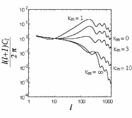
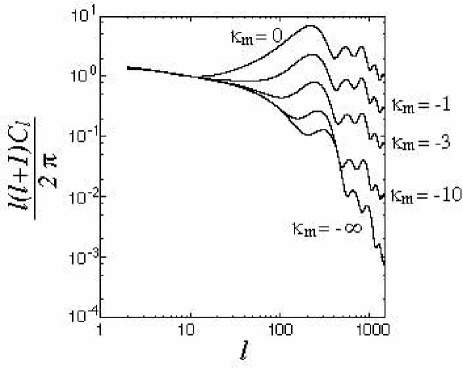
Figure 1: The CMB angular power spectra with correlated mixture of the adiabatic and isocurvature fluctuations. Here, we take $\kappa_{m}=\infty,~{}10,~{}3,~{}1,~{}0,~{}-1,~{}-3,~{}-10,~{}-\infty$. The overall normalizations are taken as $[l(l+1)C_{l}/2\pi]_{l=10}=1$.

In Fig. 1, we plot the CMB power spectrum $C_{l}$ for several values of $\kappa_{m}$ with the relation $\kappa_{\rm corr}=\kappa_{\rm iso}=\kappa_{m}$. (In our study, we use the cosmological parameters $\Omega_{b}h^{2}=0.024$, $\Omega_{m}h^{2}=0.14$, $h=0.72$, and $\tau=0.166$, where $\Omega_{b}$ and $\Omega_{m}$ are density parameters of baryon and non-relativistic matter, respectively, $h$ the Hubble constant in units of 100 km/sec/Mpc, and $\tau$ the reionization optical depth, which are suggested from the WMAP experiment [18]. We also neglect the scale dependence of $S_{i}^{(\delta\phi_{A})}$, which is expected to be small in a large class of inflationary models.) As one can see, for non-vanishing value of $\kappa_{m}$, the shape of the CMB angular power spectrum may significantly deviate from the result with the adiabatic fluctuation. Since the observed CMB angular power spectrum by the WMAP experiment is highly consistent with the prediction from the adiabatic density fluctuation, a stringent constraint on $\kappa_{\rm iso}$ and $\kappa_{\rm corr}$ can be obtained.

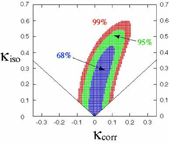
Figure 2: Probability contours for mixture of adiabatic and correlated isocurvature fluctuations. Note that we consider only the region of $\kappa_{\rm iso}\geq\left|\kappa_{\rm corr}\right|$.

As one can expect from Fig. 1, if $\kappa_{\rm iso}$ or $\kappa_{\rm corr}$ becomes too large, the CMB angular power spectrum deviates from the adiabatic result. In order to derive constraints on these parameters, we perform likelihood analysis using the WMAP data. In our analysis, we first calculate the CMB angular power spectrum for given values of $\kappa_{\rm iso}$ and $\kappa_{\rm corr}$. Then we calculate the likelihood variable using the numerical program provided by the WMAP collaboration with the WMAP data [19]. Assuming that the probability distribution is proportional to the likelihood variable, we obtain the probability distribution on the $\kappa_{\rm corr}$ vs. $\kappa_{\rm iso}$ plane, where the total probability integrated over the plane with the uniform measure is normalized to be unity (Bayesian analysis [20]).

The probability contours are shown in Fig. 2. From the figure, it is seen that $\kappa_{\rm iso}=0.4$ is allowed at 95 % C.L. for the pure (uncorrelated) isocurvature case. We can also see that a larger value of $\kappa_{\rm iso}$ is allowed if positive correlation ($\kappa_{\rm corr}>0$) exists. In the following analysis, we derive constraints on various curvaton scenarios using the result presented in Fig. 2.

4 Cosmological Moduli Fields as Curvaton

We first consider the case where the moduli fields, which are flat directions in the superstring theory, play the role of the curvaton. Interactions of the moduli fields are expected to be proportional to inverse power(s) of the gravitational scale, $M_{*}$, and their potential is lifted only by the effect of the supersymmetry breaking. If the moduli fields have non-vanishing amplitude in the early universe, they might dominate the universe at a later stage and reheat the universe when they decay. Originally, such moduli fields are considered to be cosmologically dangerous since their lifetimes may be so long that they might decay after the big-bang nucleosynthesis (BBN). In this case, the decay products of the moduli fields would spoil the success of the BBN [21]. However, it was pointed out that such a problem may be avoided if the lifetimes of the moduli fields are shorter than $\sim 1\ {\rm sec}$ [22]. This is the case if the masses of the moduli fields are heavier than about $10\ {\rm TeV}$ or so. If such cosmological moduli fields exist, they play the role of the curvaton if the primordial fluctuations are generated in the amplitudes of the moduli fields during inflation.

Let us first consider the isocurvature fluctuation in the baryonic component. In discussing the effects of the primordial fluctuation in the curvaton, we here neglect the primordial fluctuation in the baryonic sector, which may become independent and uncorrelated source of the cosmic density fluctuation. In order to parameterize the isocurvature fluctuation in the baryonic sector, we define

$$\kappa_{b}^{(\delta\phi_{A})}\equiv\left[\frac{S_{b\gamma}^{(\delta\phi_{A})}}{\Psi^{(\delta\phi_{A})}}\right]_{\rm RD2}.$$ (4.1)

Fluctuation in the baryonic sector strongly depends on when the baryon asymmetry of the universe is generated. If the baryon asymmetry is generated after the $\phi$D epoch is realized, primordial fluctuation in the curvaton is imprinted into the baryonic sector and the isocurvature fluctuation in the baryonic component does not arise. This happens when the baryon asymmetry is somehow generated from the thermally produced particles after the decay of the curvaton fields. In addition, if we consider the Affleck-Dine baryogenesis, $\kappa_{b}$ vanishes when the Affleck-Dine field starts to move after the beginning of the $\phi$D epoch. If the baryon asymmetry is generated before the $\phi$D epoch, on the contrary, fluctuation of the baryon density becomes negligibly small since baryogenesis occurs when the metric perturbations $\Psi^{(\delta\phi_{A})}$ has not grown enough. Even if there is no primordial fluctuation in the baryonic sector, however, isocurvature fluctuation may arise in the baryonic component since density fluctuation of $\hat{\phi}$ is inherited to the density fluctuation of the radiation. As we mentioned, $S_{i}$ becomes the entropy between components generated from $\phi_{i}$ and those not from $\phi_{i}$ and hence $S_{b\gamma}^{(\delta\phi_{A})}=-\sum_{i}f_{\gamma_{i}}S_{i}^{(\delta\phi_{A})}=\frac{9}{2}[\Psi^{(\delta\phi_{A})}]_{\rm RD2}$. In summary, the value of $\kappa_{b}$ depends on when the baryon asymmetry of the universe is generated:

$$\kappa_{b}=\left\{\begin{array}[]{ll}0&~{}~{}~{}:~{}~{}~{}{\rm baryogenesis\ during/after\ {\phi}D}\\ 9/2&~{}~{}~{}:~{}~{}~{}{\rm baryogenesis\ before\ {\phi}D}\end{array}\right..$$ (4.4)

Next we consider the isocurvature fluctuation in the CDM sector. One important point is that, since the interactions of the moduli fields are very weak, it is natural to expect that the reheating temperature due to the decay of the moduli fields is very low. This fact has an important implication to the scenario where the lightest supersymmetric particle (LSP) becomes the CDM since the reheating temperature may be lower than the freeze-out temperature of the LSP. If so, they should be non-thermally produced to account for the CDM. In this case fluctuations in the curvaton fields may generate extra isocurvature fluctuations in the CDM sector as will be discussed below. Of course, there are other well-motivated candidates of the CDM, like the axion, with which the isocurvature fluctuation in the CDM sector vanishes.

Let us consider the most non-trivial case where the decay products of the moduli fields directly produce the LSP [23]. In this case, the CDM density as well as the densities of the curvatons and radiation are determined by the following Boltzmann equations:

$$\frac{dn_{\tilde{\chi}_{i}}}{dt}+3Hn_{\tilde{\chi}_{i}} = \bar{N}_{\tilde{\chi},i}\Gamma_{\phi_{i}}n_{\phi_{i}}-\langle v_{\rm rel}\sigma\rangle n_{\tilde{\chi}}n_{\tilde{\chi}_{i}},$$ (4.5)

$$\frac{dn_{\phi_{i}}}{dt}+3Hn_{\phi_{i}} = -\Gamma_{\phi_{i}}n_{\phi_{i}},$$ (4.6)

$$\frac{d\rho_{\gamma_{i}}}{dt}+4H\rho_{\gamma_{i}} = (m_{\phi_{i}}-\bar{N}_{\tilde{\chi},i}m_{\tilde{\chi}})\Gamma_{\phi_{i}}n_{\phi_{i}}+m_{\tilde{\chi}}\langle v_{\rm rel}\sigma\rangle n_{\tilde{\chi}}n_{\tilde{\chi}_{i}},$$ (4.7)

where $H\equiv\dot{a}/a$, $n_{\tilde{\chi}_{i}}$ is the number density of the LSP produced from the decay of $\phi_{i}$ while $n_{\tilde{\chi}}\equiv\sum_{i}n_{\tilde{\chi}_{i}}$ is the total number density of the LSP, $m_{\tilde{\chi}}$ is the mass of the LSP, $\bar{N}_{\tilde{\chi},i}$ is the averaged number of the LSP produced in the decay of one modulus particle $\phi_{i}$, and $\langle v_{\rm rel}\sigma\rangle$ is the thermally averaged annihilation cross section of the LSP. (In our numerical calculation, we assume that the LSP is the neutral wino, as suggested by the simple anomaly mediated model. We expect that $\tilde{\chi}\tilde{\chi}\rightarrow W^{+}W^{-}$ is the dominant annihilation mode and we use

$$\langle v_{\rm rel}\sigma\rangle=\frac{g_{2}^{4}}{2\pi}\frac{1}{m_{\chi}^{2}}\frac{(1-x_{W})^{3/2}}{(2-x_{W})^{2}},$$ (4.8)

where $x_{W}\equiv m_{W}^{2}/m_{\tilde{\chi}}^{2}$ with $m_{W}$ being the $W$-boson mass, and $g_{2}$ is the gauge coupling constant of SU(2)_L. Our conclusions are qualitatively unchanged even if the LSP is not wino.)

First, we consider the case with only one (real) modulus field. (For the moment, we drop the index $i$.) Number density of the relic LSP is sensitive to the parameters $\bar{N}_{\chi}$ and $\langle v_{\rm rel}\sigma\rangle$. If $\bar{N}_{\chi}\ll 1$, the pair annihilation of the LSP becomes ineffective and hence almost all the produced LSPs survive. Then,

$$[n_{\tilde{\chi}}]_{H\sim\Gamma_{\phi}}\sim\bar{N}_{\tilde{\chi}}[n_{\phi}]_{H\sim\Gamma_{\phi}}\sim\frac{\bar{N}_{\tilde{\chi}}\Gamma_{\phi}^{2}M_{*}^{2}}{m_{\phi}},$$ (4.9)

where $n_{\phi}\equiv\rho_{\phi}/m_{\phi}$ being the number density of $\phi$, leading to

$$\frac{\rho_{c}}{s}\sim\left[\frac{m_{\tilde{\chi}}n_{\tilde{\chi}}}{T^{3}}\right]_{H\sim\Gamma_{\phi}}\sim\bar{N}_{\tilde{\chi}}\Gamma_{\phi}^{1/2}M_{*}^{1/2}\frac{m_{\tilde{\chi}}}{m_{\phi}}.$$ (4.10)

Parameterizing the decay rate of the modulus field as

$$\Gamma_{\phi}=\frac{\lambda_{\phi}^{2}}{2\pi}\frac{m_{\phi}^{3}}{M_{*}^{2}},$$ (4.11)

we obtain

$$\frac{\rho_{c}}{s}\simeq 5.8\times 10^{-6}\ {\rm GeV}\times\bar{N}_{\tilde{\chi}}\lambda_{\phi}\left(\frac{m_{\tilde{\chi}}}{100\ {\rm GeV}}\right)\left(\frac{m_{\phi}}{100\ {\rm TeV}}\right)^{1/2}\left(\frac{g_{*}}{10.75}\right)^{-1/4}.$$ (4.12)

Importantly, in this case, the resultant LSP density is insensitive to $\langle v_{\rm rel}\sigma\rangle$. On the contrary, if $\bar{N}_{\tilde{\chi}}$ becomes large enough, the pair annihilation of the LSPs cannot be neglected and the number density of the LSP is given by

$$[n_{\tilde{\chi}}]_{H\sim\Gamma_{\phi}}\sim\left[\frac{H}{\langle v_{\rm rel}\sigma\rangle}\right]_{H\sim\Gamma_{\phi}}\sim\frac{\Gamma_{\phi}}{\langle v_{\rm rel}\sigma\rangle}.$$ (4.13)

Thus, the resultant LSP density is inversely proportional to $\langle v_{\rm rel}\sigma\rangle$.

Now we discuss the density fluctuations in the multi-field case. As we discussed in the previous section, the metric perturbation is generated associated with the primordial fluctuations of the moduli fields. In discussing the cosmic density fluctuations, it is also important to understand the properties of the isocurvature fluctuations. In the RD2 epoch, behaviors of the density and metric perturbations can be understood by using Eqs. (3.21) and (3.22). Isocurvature fluctuation in the CDM sector is, on the other hand, obtained by solving Eqs. (4.5) $-$ (4.7).

In estimating the isocurvature fluctuation in the CDM sector, it is important to note that $S_{1}$ and $S_{2}$ should be different to realize a non-vanishing value of $S_{c\gamma}$. If the ratio $n_{\phi_{1}}/n_{\phi_{2}}$ does not fluctuate, the system consisting of $\phi_{1}$ and $\phi_{2}$ can be regarded as a single fluid and hence the isocurvature fluctuation should vanish. This fact implies that, if $S_{1}-S_{2}=0$, no isocurvature fluctuations can be induced as far as the components generated from the decay products of $\phi_{1}$ and $\phi_{2}$ are concerned. Thus, the isocurvature fluctuation should be proportional to $S_{12}=S_{1}-S_{2}$, and

$$S_{c\gamma}^{(\delta\phi_{A})}=\frac{\partial\ln[n_{c}/n_{\gamma}]_{\rm RD2}}{\partial\ln[n_{\phi_{1}}/n_{\phi_{2}}]_{\phi{\rm D}}}S_{12}^{(\delta\phi_{A})}.$$ (4.14)

Defining

$$\kappa_{c}^{(\delta\phi_{A})}\equiv\left[\frac{S_{c\gamma}^{(\delta\phi_{A})}}{\Psi^{(\delta\phi_{A})}}\right]_{\rm RD2},$$ (4.15)

we obtain

$$\kappa_{c}^{(\delta\phi_{A})}=-\frac{9}{2}\left[\frac{\bar{S}^{(\delta\phi_{A})}}{S_{12}^{(\delta\phi_{A})}}+\frac{1}{2}(f_{\gamma_{1}}-f_{\gamma_{2}})\right]^{-1}\frac{\partial\ln[n_{c}/n_{\gamma}]_{\rm RD2}}{\partial\ln[n_{\phi_{1}}/n_{\phi_{2}}]_{\phi{\rm D}}}.$$ (4.16)

Notice that

$$\kappa_{m}^{(\delta\phi_{A})}=(\Omega_{b}\kappa_{b}^{(\delta\phi_{A})}+\Omega_{c}\kappa_{c}^{(\delta\phi_{A})})/\Omega_{m}.$$ (4.17)

As one can see, $\kappa_{c}$, which parameterizes the size of the correlated isocurvature fluctuation in the CDM sector, depends on various parameters. First, it depends on the parameters related to the properties of the moduli fields, in particular $\Gamma_{\phi_{i}}$ and $\bar{N}_{\tilde{\chi},i}$. In addition, $\kappa_{c}$ is sensitive to the initial amplitudes of the moduli fields on which $f_{\gamma_{i}}$ depends. Furthermore, $\kappa_{c}$ depends on the transfer matrix ${\cal T}$ defined in Eq. (3.17) which parameterizes how the primordial fluctuations in the moduli fields $\delta\phi_{A}$ propagate to the fluctuations of the mass eigenstates $\delta\phi_{i}$. In particular, ${\cal T}$ determines the ratio $\bar{S}^{(\delta\phi_{A})}/S_{12}^{(\delta\phi_{A})}$. Since the interactions of the moduli fields are suppressed by inverse powers of $M_{*}$, the potential of $\hat{\phi}$ is expected to be almost parabolic if the amplitude of $\hat{\phi}$ is smaller than $M_{*}$. Then, ${\cal T}$ becomes diagonal (in some basis) with a good approximation, hence $\delta\phi_{1}$ and $\delta\phi_{2}$ become uncorrelated. In this case, $\bar{S}/S_{12}=\pm\frac{1}{2}$.

In our study, we numerically solve Eqs. (4.5) $-$ (4.7) to obtain $\kappa_{c}$ given in Eq. (4.16). Although $\kappa_{c}^{(\delta\phi_{A})}$ has complicated dependence on various parameters, we can understand its behavior for several cases if ${\cal T}$ is given by Eq. (3.18). Let us consider three extreme cases:

• $\Gamma_{\phi_{1}}\ll\Gamma_{\phi_{2}}$, $\bar{N}_{\tilde{\chi},i}\ll 1$ and $[\phi_{1}/\phi_{2}]_{\rm inf}{}^{2}\gg{\rm Max}\left[m_{\phi_{2}}^{2}/m_{\phi_{1}}^{2},~{}\bar{N}_{\tilde{\chi},2}m_{\phi_{2}}/\bar{N}_{\tilde{\chi},1}m_{\phi_{1}}\right]$:

  The decay products of $\phi_{2}$ is cosmologically negligible in this case, i.e., $f_{\gamma_{1}}\simeq 1$ and $f_{c_{1}}\simeq 1$. Therefore, no isocurvature fluctuations are generated from the fluctuation of $\phi_{1}$. On the contrary, $\delta\phi_{2}$ results in $\delta n_{\tilde{\chi}_{2}}/n_{\tilde{\chi}_{2}}\simeq\delta\rho_{\gamma_{2}}/\rho_{\gamma_{2}}\simeq S_{2}$. As a result,

  $$\kappa_{c}^{(\delta\phi_{1})}\simeq 0,~{}~{}~{}\kappa_{c}^{(\delta\phi_{2})}\simeq-\frac{9}{2}\left(\frac{f_{c_{2}}}{f_{\gamma_{2}}}-\frac{3}{4}\right).$$ (4.18)

  The ratio of the metric perturbations is given as

  $$\left|\frac{\Psi^{(\delta\phi_{2})}}{\Psi^{(\delta\phi_{1})}}\right|_{\rm RD2}=\frac{f_{\gamma_{2}}}{f_{\gamma_{1}}}\left[\frac{\phi_{1}}{\phi_{2}}\right]_{\rm inf}\simeq\left[\frac{\phi_{2}}{\phi_{1}}\right]_{\rm inf}\frac{m_{\phi_{2}}^{2}\Gamma_{\phi_{1}}^{2/3}}{m_{\phi_{1}}^{2}\Gamma_{\phi_{2}}^{2/3}}\ll 1,$$ (4.19)

  where it should be noted that the masses of the moduli fields are of the same order of magnitude as mentioned in Sec. 2. Thus $\delta\phi_{2}$ does not contribute to $\kappa_{\rm corr}$ nor $\kappa_{\rm iso}$ as long as $\bar{N}_{\tilde{\chi},1}\mathop{}_{\textstyle\sim}^{\textstyle>}\bar{N}_{\tilde{\chi},2}$, even though $\kappa_{c}^{(\delta\phi_{2})}$ is finite (see Eq. (3.32)). Thus we expect that the density fluctuation is purely adiabatic in this case. On the other hand, if $\left[\phi_{1}/\phi_{2}\right]_{\rm inf}\ll\bar{N}_{\tilde{\chi},2}m_{\phi_{2}}/\bar{N}_{\tilde{\chi},1}m_{\phi_{1}}$ is satisfied, $\kappa_{\rm iso}$ can be large due to $\delta\phi_{2}$, so the isocurvature fluctuation becomes substantial.

• $\Gamma_{\phi_{1}}\gg\Gamma_{\phi_{2}}$, $\bar{N}_{\tilde{\chi},i}\ll 1$ and $[\phi_{1}/\phi_{2}]_{\rm inf}{}^{2}\mathop{}_{\textstyle\sim}^{\textstyle>}\bar{N}_{\tilde{\chi},2}m_{\phi_{2}}/\bar{N}_{\tilde{\chi},1}m_{\phi_{1}}$:

  First we focus on the case of $[\phi_{1}/\phi_{2}]_{\rm inf}{}^{2}\gg\sqrt{m_{\phi_{2}}^{4}\Gamma_{\phi_{1}}/m_{\phi_{1}}^{4}\Gamma_{\phi_{2}}}$. In this case, most of the radiation and the CDM are generated from the decay products of $\phi_{1}$, and hence $f_{\gamma_{1}}\simeq 1$ and $f_{c_{1}}\simeq 1$. Then we obtain the same result as in the previous case;

  $$\kappa_{c}^{(\delta\phi_{1})}\simeq 0,~{}~{}~{}\kappa_{c}^{(\delta\phi_{2})}\simeq-\frac{9}{2}\left(\frac{f_{c_{2}}}{f_{\gamma_{2}}}-\frac{3}{4}\right).$$ (4.20)

  It is more interesting to consider the case of $[\phi_{1}/\phi_{2}]_{\rm inf}{}^{2}\mathop{}_{\textstyle\sim}^{\textstyle<}\sqrt{m_{\phi_{2}}^{4}\Gamma_{\phi_{1}}/m_{\phi_{1}}^{4}\Gamma_{\phi_{2}}}$. Then, most of the radiation comes from the decay of $\phi_{2}$, while most of the CDM are generated from $\phi_{1}$, namely, $f_{\gamma_{2}}\simeq 1$ and $f_{c_{1}}\simeq 1$. Thus we expect large isocurvature fluctuation.

• $\Gamma_{\phi_{1}}=\Gamma_{\phi_{2}}$ and $\bar{N}_{\tilde{\chi},i}\ll 1$:

  In this case, $\phi_{1}$ and $\phi_{2}$ simultaneously decay. Assuming $\bar{N}_{\tilde{\chi},i}\ll 1$, almost all of the CDMs produced by the decay do not experience the pair annihilation and hence the resultant number of the LSP is approximately proportional to $[\bar{N}_{\tilde{\chi},1}n_{\phi_{1}}+\bar{N}_{\tilde{\chi},2}n_{\phi_{2}}]_{H\sim\Gamma_{\phi}}$. Using the fact that $[m_{\phi_{1}}n_{\phi_{1}}+m_{\phi_{2}}n_{\phi_{2}}]_{H\sim\Gamma_{\phi}}$ is fixed, we obtain

  $$\kappa_{c}^{(\delta\phi_{1})}\simeq-\frac{9}{2f_{\gamma_{1}}}\frac{(\bar{N}_{\tilde{\chi},1}\,y-\bar{N}_{\tilde{\chi},2}x)}{(\bar{N}_{\tilde{\chi},1}+\bar{N}_{\tilde{\chi},2}\,x)(1+y)}$$ (4.21)

  where $x\equiv[n_{\phi_{2}}/n_{\phi_{1}}]_{\rm inf}$ and $y\equiv[m_{\phi_{2}}n_{\phi_{2}}/m_{\phi_{1}}n_{\phi_{1}}]_{\rm inf}$. $\kappa_{c}^{(\delta\phi_{2})}$ is obtained by replacing $1\leftrightarrow 2$ and $x,\,y\rightarrow 1/x,\,1/y$. Notice that the isocurvature fluctuation vanishes if $\bar{N}_{\tilde{\chi},1}/m_{\phi_{1}}=\bar{N}_{\tilde{\chi},2}/m_{\phi_{2}}$. This is from the fact that $\phi_{1}$ and $\phi_{2}$ can be regarded as a single fluid, since $n_{\tilde{\chi}_{1}}/n_{\gamma_{1}}=n_{\tilde{\chi}_{2}}/n_{\gamma_{2}}$ when $\bar{N}_{\tilde{\chi},1}/m_{\phi_{1}}=\bar{N}_{\tilde{\chi},2}/m_{\phi_{2}}$.

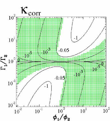
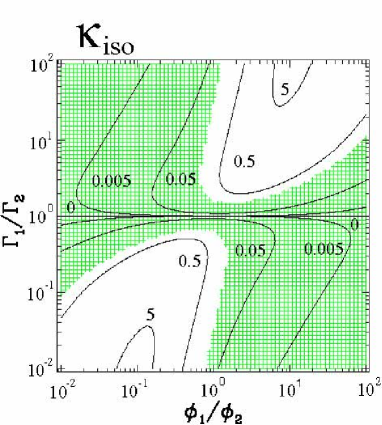
Figure 3: Contours for the values of $\kappa_{\rm iso}$ and $\kappa_{\rm corr}$ in $\Gamma_{1}/\Gamma_{2}$ vs. $[\phi_{1}/\phi_{2}]_{\rm inf}$ plane for $N_{\tilde{\chi},1}=10^{-3}$, $N_{\tilde{\chi},2}=10^{-3}$ and $\kappa_{b}=0$. We also show the allowed area within 95 % C.L. as the shaded (green) region. Here $m_{\phi_{1}}=m_{\phi_{2}}$ is assumed.

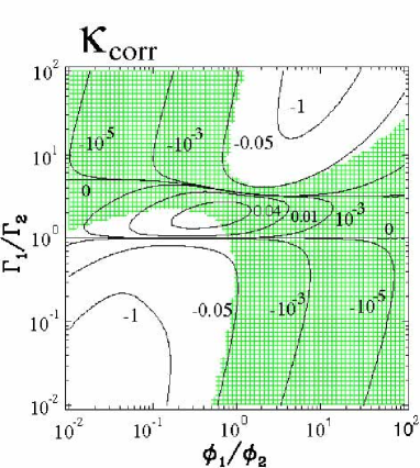
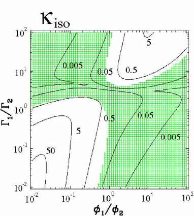
Figure 4: Same as Fig. 3 except $N_{\tilde{\chi},1}=0.1$ and $N_{\tilde{\chi},2}=10^{-3}$.

We numerically calculate $\kappa_{\rm corr}$ and $\kappa_{\rm iso}$ with the use of Eq. (3.32). Contours of constant $\kappa_{\rm corr}$ and $\kappa_{\rm iso}$ are shown in Figs. 3 and 4. Then, with $\kappa_{\rm corr}$ and $\kappa_{\rm iso}$, the CMB angular power spectrum is calculated and we derive constraints on the curvaton model under consideration making use of the likelihood analysis as Fig. 2. In the numerical calculation and the discussion hereafter, we assume $m_{\phi_{1}}=m_{\phi_{2}}$ for simplicity. Also we take $m_{\chi}=100$ GeV, and $\lambda_{\phi_{i}}^{2}$ runs from $0.1$ to $10$.

We first consider the case with $\kappa_{b}=0$. Even in this case, there are two scalar fields $\phi_{1}$ and $\phi_{2}$ and hence, in general, correlated mixture of the adiabatic and isocurvature fluctuations may arise. In order to discuss the effects of the correlated isocurvature fluctuation, we calculate the likelihood variable and derive the constraint. In Figs. 3 and 4, we plot the contours for the probabilities obtained from the likelihood analysis. The results with $N_{\tilde{\chi},1}=N_{\tilde{\chi},2}=10^{-3}$ (see Fig. 3) can be relatively easily understood. In this case, almost all the components are generated from $\phi_{1}$ when $\Gamma_{1}/\Gamma_{2}\ll 1$ and $[\phi_{1}/\phi_{2}]_{\rm inf}\gg 1$ (i.e., the lower-right corner of the figures), while the decay products of $\phi_{2}$ generates almost all the components when $\Gamma_{1}/\Gamma_{2}\gg 1$ and $[\phi_{1}/\phi_{2}]_{\rm inf}\ll 1$ (i.e., the upper-left corner of the figures). In these cases, the situation is like the case with single scalar field and hence the CMB angular power spectrum almost agrees with the adiabatic one. Remarkably, in order to realize the “adiabatic-like” result, the ratios $\Gamma_{1}/\Gamma_{2}$ and $[\phi_{1}/\phi_{2}]_{\rm inf}$ do not have to be extremely large as can be seen in Fig. 3. In the upper-right and lower-left corners of the figures, decay products of both $\phi_{1}$ and $\phi_{2}$ produce significant amount of the radiation and/or the CDM. Note that the second extreme case mentioned before cannot be seen in this figure, because $N_{\tilde{\chi},1}=N_{\tilde{\chi},2}=10^{-3}$ are not small enough and hence the pair annihilation of the LSP is not negligible. We have found that $|\kappa_{\rm corr}|$ and $\kappa_{\rm iso}$ are enhanced when the amount of the CDM from $\phi_{1}$ is comparable to that from $\phi_{2}$. In these cases, $S_{c\gamma}$ becomes sizable and the shape of the CMB angular power spectrum becomes different from that from the adiabatic fluctuations. Indeed, the CMB angular power spectrum at lower multipoles is enhanced relative to that at higher multipoles due to this effect. Furthermore, as pointed out above, one can see that the isocurvature fluctuation vanishes along the horizontal axis with $\Gamma_{1}=\Gamma_{2}$. Even if there exists large hierarchy between $N_{\tilde{\chi},1}$ and $N_{\tilde{\chi},2}$, the constraint does not change much. In Fig. 4, we plot the result for the case $N_{\tilde{\chi},1}\gg N_{\tilde{\chi},2}$.

When $\kappa_{b}\neq 0$, the constraint completely changes. As we mentioned, $\kappa_{b}=9/2$ if the baryon asymmetry is generated before the $\phi$D epoch, assuming vanishing primordial fluctuation in the baryonic component. In this case, the correlated isocurvature fluctuation almost always becomes large, leading to unacceptably large $\kappa_{\rm corr}$ and $\kappa_{\rm iso}$ irrespective of the choice of $N_{\tilde{\chi},1}$ and $N_{\tilde{\chi},2}$. Indeed, in this case, we have found that the predicted CMB angular power spectrum becomes consistent with the WMAP result in a very tiny parameter region.

Thus we conclude that mild hierarchy in $\Gamma_{1}/\Gamma_{2}$ is necessary to realize the CMB angular power spectrum consistent with the WMAP results, in the case of vanishing baryonic isocurvature fluctuation. On the other hand, if there is nonzero baryonic isocurvature fluctuation, it is difficult to obtain the CMB angular power spectrum consistent with the observations. In order to have successful curvaton scenario, we need to suppress $\kappa_{b}$ as $\kappa_{b}\mathop{}_{\textstyle\sim}^{\textstyle<}1$, which would constrain the scenario of baryogenesis.

5 Affleck-Dine Field as Curvaton

Another class of possible curvaton fields in supersymmetric models includes $F$- and $D$-flat directions. There are various flat directions in the supersymmetric models, which are lifted only by the effect of the supersymmetry breaking. One important application of such a flat direction to cosmology is the Affleck-Dine baryogenesis where baryon asymmetry of the universe originates from the condensation of such a flat direction [24]. Thus, now we consider the case where the curvaton field is one of such flat directions. In particular, in this section, we study the possibility that the Affleck-Dine field plays the role of the curvaton. In this case, the curvaton field $\hat{\phi}$ is also responsible for the baryon asymmetry of the universe. Another case will be discussed in the next section.

In the Affleck-Dine scenario, the baryon asymmetry of the universe is generated in the form of the coherent oscillation of the Affleck-Dine field. To make our discussion clearer, we adopt the following form of the potential

$$V=m_{\phi}^{2}|\hat{\phi}|^{2}+\frac{\lambda m_{\phi}^{2}}{M_{*}^{n-2}}(\hat{\phi}^{n}+{\rm h.c.}),$$ (5.1)

where the scalar field $\hat{\phi}$ has non-vanishing baryon number $B_{\phi}$. Here, since $\hat{\phi}$ is an $F$- and $D$-flat direction, $m_{\phi}$ is induced by the effect of the supersymmetry breaking and is of order the gravitino mass. In addition, $\lambda$ is a dimensionless coupling constant (which is assumed to be $O(1)$) and $n$ is an integer larger than $2$. (We choose the coefficient of the higher-dimensional operator being real using the phase rotation of $\hat{\phi}$.) We expect that the baryon-number violating term is induced from a higher dimensional Kähler interaction and hence is proportional to the parameter $m_{\phi}^{2}$. As discussed in Section 3, we assume that the potential is not affected by the Hubble-induced interactions.

The equation of motion of the Affleck-Dine field is given by

$$\ddot{\hat{\phi}}+3H\dot{\hat{\phi}}+\frac{\partial V}{\partial\hat{\phi}^{*}}=0,$$ (5.2)

which leads to

$$\dot{n}_{B}+3Hn_{B}=iB_{\phi}\left(\frac{\partial V}{\partial\hat{\phi}}\hat{\phi}-{\rm h.c.}\right),$$ (5.3)

where the baryon-number density in this case is given by $n_{B}\equiv iB_{\phi}(\hat{\phi}^{*}\dot{\hat{\phi}}-\dot{\hat{\phi}}^{*}\hat{\phi})$. Assuming non-vanishing initial amplitude, nonzero baryon number is generated when $\hat{\phi}$ starts to oscillate. The baryon number density at that moment is estimated as

$$\left[n_{B}\right]_{H\sim m_{\phi}}\sim\left[B_{\phi}{\rm Im}\left(\frac{\partial V}{\partial\hat{\phi}}\hat{\phi}\right)H^{-1}\right]_{H\sim m_{\phi}}\sim B_{\phi}\frac{\lambda m_{\phi}}{M_{*}^{n-2}}\phi_{\rm init}^{n}\sin(n\theta_{\rm init}),$$ (5.4)

where we have neglected coefficients of $O(1)$. Here, we have used the approximation that the effect of the baryon-number violating operator is so small that it can be treated as a perturbation. (Validity of such an approximation will be shown later.) As one can see, the baryon-number density becomes smaller as the initial amplitude of the Affleck-Dine field is suppressed.

The energy density of the Affleck-Dine field is given by $\rho_{\phi}\simeq m_{\phi}^{2}|\hat{\phi}|^{2}$, where we neglected the effect of the higher dimensional operator assuming $\phi_{\rm init}$ is small enough. Thus, defining

$$\epsilon\equiv\left[\frac{m_{\phi}n_{B}}{\rho_{\phi}}\right]_{\phi{\rm D}},$$ (5.5)

the $\epsilon$ parameter is given by

$$\epsilon\sim B_{\phi}\lambda\left(\frac{\phi_{\rm init}}{M_{*}}\right)^{n-2}\sin(n\theta_{\rm init}).$$ (5.6)

Importantly, when $H\mathop{}_{\textstyle\sim}^{\textstyle<}m_{\phi}$, $n_{B}$ and $\rho_{\phi}$ are both proportional to $a^{-3}$ and hence the ratio $n_{B}/\rho_{\phi}$ is a constant of time as far as $H\mathop{}_{\textstyle\sim}^{\textstyle>}\Gamma_{\phi}$. (In the case of $Q$-ball formation, $\rho_{\phi}$ and $\Gamma_{\phi}$ should be understood as the energy density and the decay rate of the $Q$-ball, respectively.)

When the Affleck-Dine field oscillates fast enough with the parabolic potential, the motion of the Affleck-Dine field is described as

$$\phi_{1}=A_{1}(t)\cos(m_{\phi}t),~{}~{}~{}\phi_{2}=A_{2}(t)\sin(m_{\phi}t),$$ (5.7)

where we have used the phase rotation of the Affleck-Dine field to obtain the above form with $A_{1}\geq A_{2}$. The amplitudes $A_{1}(t)$ and $A_{2}(t)$ are proportional to $a^{-3/2}$ when $\Gamma_{\phi}\ll H\ll m_{\phi}$.

Evaluating the ratio $n_{B}/\rho_{\phi}$ at the time of the decay of the Affleck-Dine field (or the $Q$-ball), the resultant baryon-to-entropy ratio is estimated as

$$\frac{n_{B}}{s}\sim\epsilon\frac{T_{\rm RD2}}{m_{\phi}},$$ (5.8)

where $T_{\rm RD2}$ is the reheating temperature due to the curvaton decay. In order not to spoil the success of the big-bang nucleosynthesis, $T_{\rm RD2}$ should be higher than about $1\ {\rm MeV}$ [28]. In addition, $m_{\phi}$ is as large as the gravitino mass and is expected to be smaller than $\sim 1\ {\rm TeV}$ assuming the supersymmetry as a solution to the naturalness problem in the standard model. Consequently, to explain the presently observed value of the baryon-to-entropy ratio of $n_{B}/s\sim O(10^{-10})$, the $\epsilon$ parameter should be much smaller than $1$, that is, $\epsilon\mathop{}_{\textstyle\sim}^{\textstyle<}10^{-4}$. This fact means that a large hierarchy between $A_{1}$ and $A_{2}$ is required: $|A_{2}/A_{1}|\mathop{}_{\textstyle\sim}^{\textstyle<}10^{-4}$. Such a hierarchy is realized when, for example, the initial amplitude of the Affleck-Dine field is smaller than the suppression scale of the baryon-number violating higher dimensional operator (i.e., in our example, $M_{*}$). The above fact tells us that the motion of the curvaton field is almost in the radial direction. In addition, the field $\phi_{r}$ and $\phi_{\theta}$ (almost) correspond to the mass eigenstates $\phi_{1}$ and $\phi_{2}$, respectively, since the scalar potential is well approximated by the parabolic one. As we will discuss, primordial fluctuations in $\phi_{r}$ and $\phi_{\theta}$ give rise to different type of density fluctuations.

Importantly, behaviors of the Affleck-Dine field strongly depends on the detailed shape of the potential. Even when the amplitude of $\hat{\phi}$ is small enough so that the higher dimensional interaction in Eq. (5.1) can be disregarded, the scalar potential may deviate from the simple parabolic form once the renormalization group effects are taken into account:

$$V=m_{\phi}^{2}(M_{*})\left[1+K\log(|\hat{\phi}|^{2}/M_{*}^{2})\right]|\hat{\phi}|^{2},$$ (5.9)

where we chose $M_{*}$ as a renormalization point. The parameter $K$ is from the renormalization group effect. If the Yukawa interaction associated with $\hat{\phi}$ is weak enough, the gauge interaction determines the scale dependence of $m_{\phi}$ and the parameter $K$ then becomes negative. If the Yukawa interaction becomes strong, on the contrary, $m_{\phi}^{2}$ is more enhanced at higher energy scale and the parameter $K$ becomes positive. Thus, if the Affleck-Dine mechanism works with the flat direction consisting of first and/or second generation MSSM particles, the parameter $K$ is likely to be negative. If a third generation squark (in particular, stop) or the up-type Higgs field is associated with the flat direction, however, $K$ may become positive.

Evolution of the coherent oscillation depends on the sign of $K$. If the potential of $\hat{\phi}$ is flatter than the parabolic one, coherent oscillation of the scalar field $\hat{\phi}$ may evolve into the non-topological solitonic objects called “$Q$-ball” (or in our case, “$B$-ball”) [29]. Properties of the density fluctuations differ for the cases with and without the $Q$-ball formation. Thus, we discuss these two cases separately.

5.1 Case without $Q$-ball formation

First, we consider the case where the $Q$-balls are not formed. This is the case when the parameter $K$ is positive. In this case, it is expected that the reheating temperature after the decay of the Affleck-Dine field is relatively high, i.e., higher than the freeze-out temperature of the lightest neutralino which is assumed to be the CDM. In this case, the relic LSPs are thermally produced and relic density of the LSP (more precisely, $n_{c}/s$) becomes independent of the reheating temperature due to the decay of the Affleck-Dine field. Thus, in this case, no entropy fluctuation between the CDM and the radiation is generated.

As we mentioned, when the amplitude of the Affleck-Dine field is much smaller than the suppression scale of the baryon-number violating higher dimensional interactions, the fields $\phi_{r}$ and $\phi_{\theta}$ (almost) correspond to the mass eigenstates $\phi_{1}$ and $\phi_{2}$, respectively. Primordial fluctuations in $\phi_{r}$ and $\phi_{\theta}$ result in different type of density fluctuations. Because of the large hierarchy between the amplitude of the fields $\phi_{1}\simeq\phi_{r}$ and $\phi_{2}\simeq\phi_{\theta}$, almost all the photons in the RD2 epoch are generated from the decay products of $\phi_{1}$ and hence $f_{\gamma_{1}}\simeq 1$ while $f_{\gamma_{2}}\simeq 0$. Furthermore, since the Affleck-Dine field mostly feels the parabolic potential, the primordial entropy fluctuations are given by

$$S_{i}=\left[\frac{2\delta\phi_{i}}{\phi_{i}}\right]_{\rm inf}.$$ (5.10)

As a result, using Eq. (3.22), we obtain

$$\left[\Psi^{(\delta\phi_{r})}\right]_{\rm RD2}\simeq-\frac{4}{9}\frac{\delta\phi_{r}}{\phi_{\rm init}},~{}~{}~{}\left[\Psi^{(\delta\phi_{\theta})}\right]_{\rm RD2}\simeq 0.$$ (5.11)

In addition, since $\delta\phi_{r}$ and $\delta\phi_{\theta}$ provide fluctuations in $\phi_{\rm init}$ and $\theta$, respectively, the entropy fluctuation between the baryon and radiation is also expected. Indeed, using the fact that the $\epsilon$ parameter given in Eq. (5.5) is proportional to the resultant baryon-to-entropy ratio, entropy fluctuation in the baryonic sector is estimated:

$$S_{b\gamma}^{(\delta\phi_{r})}=(n-2)\frac{\delta\phi_{r}}{\phi_{\rm init}},~{}~{}~{}S_{b\gamma}^{(\delta\phi_{\theta})}=n\cot(n\theta_{\rm init})\frac{\delta\phi_{\theta}}{\phi_{\rm init}}.$$ (5.12)

Since the fluctuations $\delta\phi_{r}$ and $\delta\phi_{\theta}$ are uncorrelated, the total CMB angular power spectrum is given by a linear combination of the two power spectra $C_{l}^{(\delta\phi_{r})}$ and $C_{l}^{(\delta\phi_{\theta})}$, which are characterized by the following $\kappa_{m}$ parameters:

$$\kappa_{m}^{(\delta\phi_{r})}\simeq-\frac{9}{4}\frac{(n-2)\Omega_{b}}{\Omega_{m}},~{}~{}~{}\kappa_{m}^{(\delta\phi_{\theta})}\simeq\infty.$$ (5.13)

Thus, the CMB angular power spectrum associated with $\delta\phi_{\theta}$ is (almost) the same as the purely isocurvature result while $C_{l}^{(\delta\phi_{r})}$ is from the correlated mixture of the adiabatic and isocurvature fluctuations. Relative size of $C_{l}^{(\delta\phi_{r})}$ and $C_{l}^{(\delta\phi_{\theta})}$ depends on $\theta_{\rm init}$. Since $\kappa_{m}^{(\delta\phi_{r})}<0$, however, the acoustic peaks are always suppressed compared to the adiabatic case once one normalizes the Sachs-Wolfe tail. Since the angular power spectrum measured by the WMAP is well consistent with the adiabatic result, suppression of the acoustic peaks causes discrepancy between the theoretical prediction and the observations. To study this issue, in Fig. 5, we plot the predicted CMB angular power spectrum for the case with $n=4$ normalizing the Sachs-Wolfe tail. Here, we use the relation (5.13) with $\cot n\theta_{\rm init}=0$ which makes the discrepancy smallest. As one can see, even in the case with $\cot n\theta_{\rm init}=0$, the CMB angular power spectrum becomes extremely inconsistent with the WMAP results. Indeed, the total angular power spectrum is characterized by the following $\kappa$ parameters:

$$\kappa_{\rm corr}\simeq-\frac{9}{4}\frac{(n-2)\Omega_{b}}{\Omega_{m}},~{}~{}~{}\kappa_{\rm iso}\simeq\frac{9}{4}\frac{\Omega_{b}}{\Omega_{m}}\sqrt{(n-2)^{2}+n^{2}\cot^{2}\left(n\theta_{\rm init}\right)},$$ (5.14)

and, using $n\geq 3$ and adopting our canonical values of $\Omega_{b}$ and $\Omega_{m}$, we obtain $\kappa_{\rm corr}\mathop{}_{\textstyle\sim}^{\textstyle<}-0.39$ and $|\kappa_{\rm iso}|>0.39$, which is inconsistent with the observational results. (See Fig. 2).

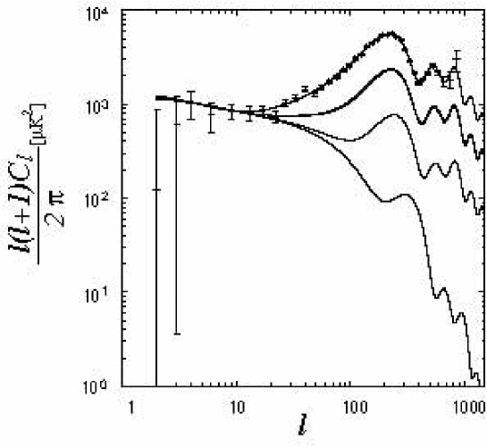
Figure 5: The predicted CMB angular power spectra for the case where the Affleck-Dine field plays the role of the curvaton. From top to bottom, the WMAP data and the best-fit $\Lambda$CDM model, the case without the $Q$-ball formation, the case with the $Q$-ball formation ($C=1$) which accidentally coincides with the previous case, the case with the $Q$-ball formation ($C=0$), and the purely isocurvature case. We take $n=4$, $\cot n\theta_{\rm init}=0$ and normalize the Sachs-Wolfe tail.

Therefore, the present case is excluded by the WMAP result. As we have shown, this is due to too large entropy fluctuation in the baryonic sector [30]. We should emphasize that the result obtained here is quite generic, independently of the detailed dynamics of the Affleck-Dine mechanism as far as the Affleck-Dine field is an $F$- and $D$-flat direction. Thus, we conclude that the Affleck-Dine field cannot play the role of the curvaton. In the next subsection, we will see that essentially the same conclusion is obtained for the case with the $Q$-ball formation.

5.2 Case with $Q$-ball formation

If the potential of the Affleck-Dine field is flatter than the parabolic one, it is inevitable that the $Q$-balls are formed. This is due to the fact that, if $K<0$, instability band arises in the momentum space, which is given by

$$0<k_{\rm phys}^{2}<2m_{\phi}^{2}|K|,$$ (5.15)

where $k_{\rm phys}$ is the physical momentum. In this case, once the Affleck-Dine field starts to oscillate, fluctuation with the momentum within the instability band grows rapidly.

Typical initial charge of the $Q$-ball generated in this process depends on the value of $\epsilon$. If $\epsilon$ is close to 1, charge of the typical $Q$-ball is given by the total charge within the horizon at the time of the $Q$-ball formation. As a result, typical initial charge $|Q|_{\rm init}$ is proportional to $\epsilon$. In this case, formation of the $Q$-ball with opposite sign of charge (so-called anti-$Q$-ball) is ineffective. If $\epsilon$ becomes much smaller than 1, however, $|Q|_{\rm init}$ becomes independent of $\epsilon$. In this case, almost same number of the $Q$-ball and anti-$Q$-ball are formed with the relation $\epsilon=(n_{Q}-n_{\bar{Q}})/(n_{Q}+n_{\bar{Q}})$, where $n_{Q}$ and $n_{\bar{Q}}$ are the number densities of the $Q$-ball and anti-$Q$-ball, respectively. Indeed, numerical lattice simulations have shown that

$$|Q|_{\rm init}\sim\bar{\beta}_{n}\left(\frac{\phi_{\rm init}}{m_{\phi}}\right)^{2}\times\left\{\begin{array}[]{ll}\epsilon{}{}{}&~{}~{}~{}{\rm for}\ \epsilon\mathop{}_{\textstyle\sim}^{\textstyle>}\epsilon_{\rm c}\\ \epsilon_{\rm c}{}{}{}&~{}~{}~{}{\rm for}\ \epsilon\mathop{}_{\textstyle\sim}^{\textstyle<}\epsilon_{\rm c}\end{array}\right.,$$ (5.18)

where $\bar{\beta}_{n}\sim 6\times 10^{-3}$ and $\epsilon_{\rm c}\sim 0.01$ [31].

In addition, the condition for the instability band (5.15) provides the size of the $Q$-ball as

$$R_{Q}\sim\frac{1}{|K|^{1/2}m_{\phi}}.$$ (5.19)

As long as the initial value of the $Q$-ball charge is larger than $O(10^{18})$, evaporation of the $Q$-ball is ineffective and the universe is reheated by the decay of the $Q$-ball. The decay process of a single $Q$-ball is described by

$$\dot{Q}\sim-\frac{m_{\phi}^{3}{\cal A}}{192\pi^{2}},$$ (5.20)

where ${\cal A}=4\pi R_{Q}^{2}$ is the surface area of the $Q$-ball [33]. (This relation is valid when the charge of the $Q$-ball is much larger than 1.) Thus, in our case, $\dot{Q}$ is (almost) a constant of time and hence the lifetime of the $Q$-ball with initial charge $Q_{\rm init}$ is given by $\Gamma_{Q}^{-1}\sim|Q_{\rm init}/\dot{Q}|$. Using Eq. (5.18) with $\epsilon\mathop{}_{\textstyle\sim}^{\textstyle<}\epsilon_{c}$, the decay temperature of the $Q$-ball, i.e., $T_{\rm RD2}$, is estimated as

$$T_{\rm RD2}\sim 1\ {\rm MeV}\times\left(\frac{|K|}{0.03}\right)^{-1/2}\left(\frac{m_{\phi}}{1{\rm TeV}}\right)^{3/2}\left(\frac{\phi_{\rm init}}{M_{*}}\right)^{-1}.$$ (5.21)

One of important consequences of the $Q$-ball formation is that the RD2 epoch may be realized at much lower temperature compared to the case without $Q$-ball formation; for the $Q$-ball charge $Q_{\rm init}\sim 10^{21}-10^{27}$, the RD2 epoch is realized at the temperature $T_{\rm RD2}\sim 1\ {\rm MeV}-1\ {\rm GeV}$, which is lower than the freeze-out temperature of the lightest neutralino (which is assumed to be the LSP). The other important consequence is that the decay rate of $Q$-balls, $\Gamma_{Q}$, can be another source of the density fluctuations [34]. Note that $\Gamma_{Q}$ depends on $\phi_{\rm init}$, and that the decay process is different from the usual exponential decay. Hence, if $\phi_{\rm init}$ fluctuates spatially, $\Gamma_{Q}$ has spatial variation, leading to additional density fluctuations.

Now we discuss the density fluctuation in the case with $Q$-ball formation. First, we consider the metric perturbation. Taking account of the fact that fluctuation of the decay rate generates adiabatic density perturbation [34], the metric perturbation has the following form:

$$\left[\Psi^{(\delta\phi_{r})}\right]_{\rm RD2}\simeq-\left(\frac{4}{9}+C\right)\frac{\delta\phi_{r}}{\phi_{\rm init}},~{}~{}~{}\left[\Psi^{(\delta\phi_{\theta})}\right]_{\rm RD2}\simeq 0,$$ (5.22)

where the second term in $\Psi^{(\delta\phi_{r})}$ represents the contribution due to the varying decay rate, and the typical value of $C$ is estimated to be order of unity. For our purpose, it is not necessary to know the precise value of $C$, but we crudely set $C=1$. As long as $C\sim O(1)$, our conclusion does not change. Note that its sign is determined by the fact that the lifetime of $Q$-balls becomes longer for larger $\phi_{\rm init}$, leading to more negative gravitational potential. Next we consider the isocurvature fluctuation in the baryonic and CDM sector. Since the density fluctuation due to the varying decay rate does not change entropy perturbations, we take $\Gamma_{Q}$ constant in the following. While the baryonic isocurvature fluctuation is calculated as in the previous subsection, the property of $\delta_{c}$ can be different from the case without $Q$-ball formation.

To discuss the isocurvature fluctuation in the CDM sector, it is important to understand how the relic density of the lightest neutralino (i.e., the CDM density) is determined. If $T_{\rm RD2}$ is lower than the freeze-out temperature of the LSP, the relic abundance of the LSP is non-thermally determined. The relic abundance depends on whether the annihilation rate of the LSP at the decay is larger or smaller than the expansion rate of the universe. If the annihilation rate is smaller than the expansion rate, (almost) all the LSPs produced by the decay of the $Q$-ball survive. In this case, no entropy fluctuation is expected between the LSP (i.e., the CDM) and the photon produced by the $Q$-ball decay. If all the LSPs produced by the $Q$-ball survives, however, the relic density of the LSP is expected to become much larger than the critical density of the universe. This is because the $Q$-ball consists of the condensation of supersymmetric particles (i.e., the scalar quarks and/or scalar leptons) and hence the situation corresponds to the case discussed in Section 4 with $\bar{N}_{\tilde{\chi}}\sim 0.1-1$. Indeed, from Eq. (4.10), we can estimate the LSP density normalized by the entropy density of the universe:

$$\frac{\rho_{c}}{s} \simeq 10^{-5}{\rm GeV}\left(\frac{\bar{N}_{\tilde{\chi}}}{0.1}\right)\left(\frac{T_{\rm RD2}}{1{\rm MeV}}\right)\left(\frac{m_{\tilde{\chi}}}{100{\rm GeV}}\right)\left(\frac{m_{\phi}}{1{\rm TeV}}\right)^{-1},$$ (5.23)

which is much larger than the observed value $\rho_{\rm crit}/s\simeq 3.6\times 10^{-9}h^{2}{\rm GeV}$, with $\rho_{\rm crit}$ being the critical density of the universe.

Thus, in the following we discuss the case where the annihilation rate of the LSP is larger than the expansion rate of the universe. In this case, the pair annihilation proceeds until the annihilation rate becomes comparable to the expansion rate and hence $[n_{\tilde{\chi}}]_{\rm H\sim\Gamma_{Q}}\sim\Gamma_{Q}/\langle v_{\rm rel}\sigma\rangle$. In the RD2 epoch or later, ratio of $n_{\tilde{\chi}}$ to $n_{\gamma}$ is conserved and hence we obtain

$$\frac{n_{\tilde{\chi}}}{n_{\gamma}}\sim\frac{1}{T_{\rm RD2}M_{*}\langle v_{\rm rel}\sigma\rangle},$$ (5.24)

where we have used the relation $\Gamma_{Q}\sim T_{\rm RD2}^{2}/M_{*}$. We assume that $\Gamma_{Q}$ and $\langle v_{\rm rel}\sigma\rangle$ satisfy the relation such that the above ratio becomes consistent with the currently observed dark matter density [25].

As shown in Eq. (5.21), $T_{\rm RD2}$ depends on $\phi_{\rm init}$ and hence the ratio $n_{\tilde{\chi}}/n_{\gamma}$ fluctuates if the Affleck-Dine field has primordial fluctuation. Using $T_{\rm RD2}\propto\phi_{\rm init}^{-1}$, we obtain $n_{\tilde{\chi}}/n_{\gamma}\propto\phi_{\rm init}$. Then,

$$S_{c\gamma}^{(\delta\phi_{r})}=\frac{\delta\phi_{r}}{\phi_{\rm init}},~{}~{}~{}S_{c\gamma}^{(\delta\phi_{\theta})}=0,$$ (5.25)

where we have used the relation $S_{c\gamma}=\delta(n_{c}/n_{\gamma})/(n_{c}/n_{\gamma})$. In this case, the fluctuation in the radial direction, $\delta\phi_{r}$, also generates the isocurvature fluctuation in the CDM sector. Notice that the fluctuation in the phase direction $\delta\phi_{\theta}$ does not affect the isocurvature fluctuation in the CDM since $\epsilon\ll 1$.

In the case of the $Q$-ball formation, significant amount of the isocurvature fluctuations are generated associated with $\delta\phi_{r}$ and $\delta\phi_{\theta}$. Adding the isocurvature fluctuations in the baryon and the CDM, we obtain

$$\kappa_{m}^{(\delta\phi_{r})}\simeq-\left(\frac{4}{9}+C\right)^{-1}\frac{(n-2)\Omega_{b}+\Omega_{c}}{\Omega_{m}},~{}~{}~{}\kappa_{m}^{(\delta\phi_{\theta})}\simeq\infty.$$ (5.26)

Importantly, $\kappa_{m}^{(\delta\phi_{r})}$ is again negative and $\kappa_{m}^{(\delta\phi_{\theta})}\gg 1$. Thus, $\delta\phi_{r}$ results in the density fluctuations with correlated mixture of the adiabatic and isocurvature fluctuations while $\delta\phi_{\theta}$ becomes (almost) purely isocurvature fluctuations. The $\kappa$ parameters, which characterize the total CMB power spectrum, are thus given by

$$\kappa_{\rm corr} \simeq -\left(\frac{4}{9}+C\right)^{-1}\frac{(n-2)\Omega_{b}+\Omega_{c}}{\Omega_{m}},$$

$$\kappa_{\rm iso} \simeq \left(\frac{4}{9}+C\right)^{-1}\Omega_{m}^{-1}\sqrt{((n-2)\Omega_{b}+\Omega_{c})^{2}+(n\cot\left(n\theta_{\rm init}\right)\Omega_{b})^{2}}.$$ (5.27)

For the total CMB angular power spectrum, if one normalizes the Sachs-Wolfe tail, acoustic peaks are extremely suppressed compared to the purely adiabatic case. In Fig. 5, the CMB angular power spectrum with the relation Eq. (5.2) is also plotted in the case of $\cot n\theta_{\rm init}=0$ and $C=0$ and $1$. In this case, again, the shape of the total CMB angular power spectrum becomes inconsistent with the observations.

To summarize, the Affleck-Dine field cannot be the curvaton in both of the cases with and without $Q$-ball formation because the entropy density fluctuation in baryonic and/or CDM sector is too large. In other words, if Affleck-Dine field (or $Q$-ball) dominates the energy density of the universe, its primordial fluctuation must be suppressed, and the dominant density fluctuation must be generated by another source, like inflaton.

6 $F$- and $D$-Flat Direction as Curvaton

In this section, we consider the case where an $F$- and $D$-flat direction plays the role of curvaton which is not related to the mechanism of baryogenesis. Even in this case, $Q$-ball may or may not be produced depending on the shape of the curvaton potential; in particular, if the curvaton potential is flatter than parabolic (which may be due to the renormalization effects), $Q$-ball can be produced once the curvaton starts to oscillate. As can be expected from the discussion given in the previous section, properties of the cosmological density fluctuations strongly depend on how the curvaton field evolves.

First, let us consider the simplest possibility, namely, the case without the $Q$-ball formation. In this case, $T_{\rm RD2}$ is expected to be higher than the freeze out temperature of the lightest supersymmetric particle and we assume that the CDM is thermally produced lightest neutralino. If $T_{\rm RD2}$ is high enough, baryogenesis may be possible with the decay products of $\hat{\phi}$. For example, the Fukugita-Yanagida mechanism [35] using the decay of thermally produced right-handed neutrinos may work if $T_{\rm RD2}\mathop{}_{\textstyle\sim}^{\textstyle>}10^{9-10}~{}{\rm GeV}$ [36]. Another possibility may be electroweak baryogenesis [37] if $T_{\rm RD2}\mathop{}_{\textstyle\sim}^{\textstyle>}100\ {\rm GeV}$.

In this simplest case, no isocurvature fluctuation between the non-relativistic components and the radiation is generated by $\delta\phi_{r}$ nor $\delta\phi_{\theta}$ (i.e., $\kappa_{m}=0$). Thus, in the RD2 epoch, the only source of the cosmic density fluctuations is the metric perturbation given in Eq. (3.22). Since no isocurvature fluctuation is generated, $C_{l}^{(\delta\phi_{r})}$ and $C_{l}^{(\delta\phi_{\theta})}$ are both from purely adiabatic density fluctuations and hence $C_{l}^{(\delta\phi_{r})}\propto C_{l}^{(\delta\phi_{\theta})}$. Thus, even though $\Psi^{(\delta\phi_{r})}$ and $\Psi^{(\delta\phi_{\theta})}$ are free parameters, it does not affect the shape of the total CMB angular power spectrum and $C_{l}$ is the same as the result with purely-adiabatic scale-invariant primordial density fluctuations. (Concrete models for the flat-direction curvaton is found in Ref. [38].)

As discussed in the previous section, if the scalar potential of the flat direction field is flatter than the parabolic one, the $Q$-balls are formed. If the initial charge of the $Q$-ball is small enough, it decays (or evaporates) with a temperature above the freeze-out temperature of the LSP. This case is reduced to the one discussed just above, where the purely-adiabatic density fluctuation is obtained. If the charge of the $Q$-ball is large, however, it decays after the thermal pair-annihilation of the LSPs are frozen out. Thus, one can see that the entropy fluctuation is generated in the CDM sector:

$$S_{c\gamma}^{(\delta\phi_{r})}=\frac{\delta\phi_{r}}{\phi_{\rm init}},~{}~{}~{}S_{c\gamma}^{(\delta\phi_{\theta})}=0,$$ (6.1)

which leads to

$$\kappa_{m}^{(\delta\phi_{r})}\simeq-\left(\frac{4}{9}+C\right)^{-1}\frac{\Omega_{c}}{\Omega_{m}},~{}~{}~{}\kappa_{m}^{(\delta\phi_{\theta})}=0,$$ (6.2)

where $C\sim O(1)$ represents the contribution due to the varying decay constant. Notice that there is no baryonic entropy fluctuation, since the curvaton has nothing to do with baryon asymmetry. In this case, $\left|\Psi^{(\delta\phi_{\theta})}\right|\ll\left|\Psi^{(\delta\phi_{r})}\right|$ and hence $\delta\phi_{\theta}$ does not play any significant role in generating the cosmic density fluctuations. Thus, with the best-fit values of $\Omega_{c}$ and $\Omega_{m}$ obtained from the WMAP experiment, $\kappa_{\rm corr}\simeq-1.9,-0.57$ for $C=0,1$ respectively, which are clearly excluded by the observation. (See Fig. 2). Therefore, again, the curvaton with $Q$-ball formation which decays after the freeze-out of the LSP is rejected.

7 Right-Handed Sneutrino as Curvaton

Recent neutrino-oscillation experiments strongly suggest tiny but non-vanishing masses of the neutrinos. Such small masses can be naturally explained by introducing the right-handed neutrinos [39].

If the right-handed neutrino exists in supersymmetric models, its superpartner may have non-vanishing primordial amplitude. In particular, such a case has been studied related to the possibility of generating the lepton number (and baryon number) asymmetry of the universe from the decay product of the right-handed sneutrino [40]. In this case, the right-handed sneutrino can be an another candidate for the curvaton [41].

The scenario with the right-handed sneutrino condensation is almost the same as the previous cases except for the origin of the baryon asymmetry of the universe. During inflation, the right-handed sneutrino is assumed to have a non-vanishing amplitude. After inflation, the right-handed sneutrino starts to oscillate when the expansion rate of the universe becomes comparable to the sneutrino mass $m_{\phi}$. If the decay of the oscillating right-handed sneutrino takes place much later than the inflaton decay, the sneutrino dominates the universe. Then, the sneutrino decays when the expansion rate of the universe becomes comparable to its decay rate. At the time of the decay, lepton number asymmetry can be generated provided that CP violation exists in the neutrino sector. Once the lepton number asymmetry is generated, it can be converted to the baryon number asymmetry due to the sphaleron process [37].

In this scenario, quantum fluctuations that the sneutrino acquires during inflation accounts for the adiabatic density fluctuations and hence the right-handed sneutrino plays the role of the curvaton. Here, baryon asymmetry of the universe is generated from the decay products of the right-handed sneutrino and hence no isocurvature fluctuation is expected in the baryonic sector. In addition, the decay rate of the right-handed sneutrino is high enough so that the LSPs (and other superpartners of the standard-model particles) are thermally produced. Then there is no isocurvature fluctuation in the CDM sector if the LSP becomes the CDM.

If this is the case, the primordial density fluctuations become purely adiabatic and hence the resultant CMB angular power spectrum becomes well consistent with the results of the WMAP experiment. Thus, we conclude that the right-handed sneutrino is one of the good and well-motivated candidates for the curvaton.

8 Conclusions and Discussion

We have studied several candidates for the curvaton in the supersymmetric framework. Since scalar fields appearing in supersymmetric models are inevitably complex, it is necessary to consider cases with multi-curvaton fields. In this case, primordial fluctuations in the curvatons induce isocurvature (entropy) fluctuations as well as the adiabatic ones. Such isocurvature fluctuations may affect the CMB angular power spectrum and the recent WMAP experiment sets stringent constraints on those models.

One potential problem of the curvaton scenario in the supersymmetric models is to suppress the baryonic isocurvature fluctuations. As shown in the present paper, isocurvature fluctuation in the baryonic sector may arise in various situations. In many cases, such a baryonic isocurvature becomes too large to be consistent with the WMAP result.

Besides baryonic isocurvature fluctuations, we have found that the CDM isocurvature fluctuations are important for moduli or $Q$-ball curvaton where the abundance of the dark matter (i.e., the LSP) is determined non-thermally and hence its fluctuations are isocurvature with correlation to the curvaton fluctuations.

If the cosmological moduli fields play the role of the curvaton, it is possible that the reheating temperature due to the decay of the moduli fields is lower than the freeze-out temperature of the lightest neutralino. In this case, the CDM is non-thermally produced if the lightest neutralino is the CDM, and the entropy fluctuation between the two curvatons (i.e., the real and imaginary parts of the curvaton) in general becomes the isocurvature fluctuation in the CDM sector. This fact excludes some part of the parameter space but, as we have seen, slight hierarchies between the initial amplitudes and/or the decay rates of two curvaton fields are enough to make the resultant CMB anisotropy consistent with the WMAP result. Of course, if the lightest neutralino is not the CDM, then we may evade the constraint from the isocurvature fluctuation in the CDM sector. An example for such CDM candidates is axion.

If the Affleck-Dine field becomes the curvaton, on the contrary, too large baryonic isocurvature fluctuation is inevitably induced. As we have seen, the acoustic peaks are always too much suppressed to be consistent with the observations if the Affleck-Dine field plays the role of the curvaton. Thus, the Affleck-Dine field cannot play the role of the curvaton. It is also notable that, in the case with $Q$-ball formation, extra isocurvature fluctuation may arise if the reheating temperature due to the $Q$-ball decay is lower than the freeze-out temperature of the lightest neutralino (which is assumed to be the CDM).

For the case where the $F$- and $D$-flat direction (without baryon number) becomes the curvaton, isocurvature fluctuation in the CDM sector may also arise if the $Q$-ball is formed. In this case, the resultant CMB angular power spectrum is too much affected by the isocurvature fluctuation. Without the $Q$-ball formation, however, the $F$- and $D$-flat direction (but not the Affleck-Dine field) can be a candidate of the curvaton.

Another good and well-motivated candidate of the curvaton is the right-handed sneutrino. If the right-handed sneutrino acquires the primordial quantum fluctuations during inflation, it becomes purely adiabatic density fluctuations and the resultant CMB angular power spectrum can be well consistent with the WMAP result.

In summary, for a viable scenario of the curvaton, the isocurvature contribution should be so small that the CMB angular power spectrum becomes consistent with the WMAP result. In the supersymmetric case, this fact provides stringent constraints on the curvaton scenario. Thus, it is necessary to look for curvaton candidates which do not generate the isocurvature fluctuations; some of them are already found in the present study.

Acknowledgments: We acknowledge the use of CMBFAST [42] package for our numerical calculations. The work of T.M. is supported by the Grant-in-Aid for Scientific Research from the Ministry of Education, Science, Sports, and Culture of Japan, No. 15540247. K.H. and F.T. thank the Japan Society for the Promotion of Science for financial support.

References

- [1] D. N. Spergel et al., arXiv:astro-ph/0302209; A. Kogut et al., arXiv:astro-ph/0302213; G. Hinshaw et al., arXiv:astro-ph/0302217; L. Verde et al., arXiv:astro-ph/0302218; H. V. Peiris et al., arXiv:astro-ph/0302225.
- [2] K. Enqvist and M. S. Sloth, Nucl. Phys. B 626 (2002) 395.
- [3] D. H. Lyth and D. Wands, Phys. Lett. B 524 (2002) 5.
- [4] T. Moroi and T. Takahashi, Phys. Lett. B 522 (2001) 215 [Erratum-ibid. B 539 (2002) 303]; Phys. Rev. D 66 (2002) 063501.
- [5] D. H. Lyth, C. Ungarelli and D. Wands, Phys. Rev. D 67 (2003) 023503.
- [6] S. Mollerach, Phys. Rev. D 42 (1990) 313; A. D. Linde and V. Mukhanov, Phys. Rev. D 56 (1997) 535.
- [7] N. Bartolo and A. R. Liddle, Phys. Rev. D 65 (2002) 121301; M. S. Sloth, Nucl. Phys. B 656 (2003) 239; R. Hofmann, arXiv:hep-ph/0208267; K. Dimopoulos and D. H. Lyth, arXiv:hep-ph/0209180; T. Moroi and H. Murayama, Phys. Lett. B 553 (2003) 126; K. Enqvist, S. Kasuya and A. Mazumdar, Phys. Rev. Lett. 90 (2003) 091302; F. Di Marco, F. Finelli and R. Brandenberger, Phys. Rev. D 67 (2003) 063512; K. A. Malik, D. Wands and C. Ungarelli, Phys. Rev. D 67 (2003) 063516; M. Postma, Phys. Rev. D 67 (2003) 063518; C. Gordon and A. Lewis, arXiv:astro-ph/0212248; K. Dimopoulos, arXiv:astro-ph/0212264; A. R. Liddle and L. A. Urena-Lopez, arXiv:astro-ph/0302054; J. McDonald, arXiv:hep-ph/0302222; K. Dimopoulos, G. Lazarides, D. Lyth and R. Ruiz de Austri, arXiv:hep-ph/0303154; K. Enqvist, A. Jokinen, S. Kasuya and A. Mazumdar, arXiv:hep-ph/0303165; K. Dimopoulos, D. H. Lyth, A. Notari and A. Riotto, arXiv:hep-ph/0304050; M. Endo, M. Kawasaki and T. Moroi, arXiv:hep-ph/0304126; M. Postma and A. Mazumdar, arXiv:hep-ph/0304246; M. Postma, arXiv:astro-ph/0305101; S. Kasuya, M. Kawasaki and F. Takahashi, arXiv:hep-ph/0305134. D. H. Lyth and D. Wands, arXiv:astro-ph/0306498; D. H. Lyth and D. Wands, arXiv:astro-ph/0306500; K. Dimopoulos, G. Lazarides, D. Lyth and R. R. de Austri, arXiv:hep-ph/0308015; J. McDonald, arXiv:hep-ph/0308048.
- [8] G. Veneziano, Phys. Lett. B 265 (1991) 287; M. Gasperini and G. Veneziano, Astropart. Phys. 1 (1993) 317; M. Gasperini and G. Veneziano, Phys. Rev. D 50 (1994) 2519.
- [9] M. Gasperini and G. Veneziano, Phys. Rep. 373 (2003) 1.
- [10] J. Khoury, B. A. Ovrut, P. J. Steinhardt and N. Turok, Phys. Rev. D 64 (2001) 123522; J. Khoury, B. A. Ovrut, N. Seiberg, P. J. Steinhardt and N. Turok, Phys. Rev. D 65 (2002) 086007; J. Khoury, B. A. Ovrut, P. J. Steinhardt and N. Turok, Phys. Rev. D 66 (2002) 046005.
- [11] D.H. Lyth, Phys. Lett. B 524 (2002) 1; R. Brandenberger, F. Finelli, JHEP 0111 (2001) 056; J. Hwang, Phys. Rev. D 65 (2002) 063514.
- [12] E. Halyo, Phys. Lett. B 387 (1996) 43; P. Binetruy and G. R. Dvali, Phys. Lett. B 388 (1996) 241.
- [13] M. K. Gaillard, H. Murayama and K. A. Olive, Phys. Lett. B 355 (1995) 71.
- [14] L. Randall and R. Sundrum, Nucl. Phys. B 557 (1999) 79.
- [15] G. F. Giudice, M. A. Luty, H. Murayama and R. Rattazzi, JHEP 9812 (1998) 027.
- [16] J. A. Bagger, T. Moroi and E. Poppitz, JHEP 0004 (2000) 009.
- [17] W. T. Hu, Ph.D thesis (astro-ph/9508126).
- [18] D.N. Spergel et al. in Ref. [1].
- [19] L. Verde et al., G. Hinshaw et al. and A. Kogut et al. in Ref. [1].
- [20] K. Hagiwara et al. [Particle Data Group Collaboration], Phys. Rev. D 66 (2002) 010001.
- [21] G. D. Coughlan, W. Fischler, E. W. Kolb, S. Raby and G. G. Ross, Phys. Lett. B 131 (1983) 59; T. Banks, D. B. Kaplan and A. E. Nelson, Phys. Rev. D 49 (1994) 779; B. de Carlos, J. A. Casas, F. Quevedo and E. Roulet, Phys. Lett. B 318 (1993) 447.
- [22] T. Moroi, M. Yamaguchi and T. Yanagida, Phys. Lett. B 342 (1995) 105; M. Kawasaki, T. Moroi and T. Yanagida, Phys. Lett. B 370 (1996) 52.
- [23] T. Moroi and L. Randall, Nucl. Phys. B 570 (2000) 455.
- [24] I. Affleck and M. Dine, Nucl. Phys. B 249 (1985) 361.
- [25] M. Fujii and K. Hamaguchi, Phys. Lett. B 525 (2002) 143; Phys. Rev. D 66 (2002) 083501.
- [26] M. Dine, A.E. Nelson and Y. Shirman, Phys. Rev. D 51 (1995) 1362; M. Dine, A.E. Nelson, Y. Nir and Y. Shirman, Phys. Rev. D 53 (1996) 2658.
- [27] G.R. Dvali, A. Kusenko and M.E. Shaposhnikov, Phys. Lett. B 417 (1998) 99; A. Kusenko and M.E. Shaposhnikov, Phys. Lett. B 418 (1998) 46.
- [28] M. Kawasaki, K. Kohri and N. Sugiyama, Phys. Rev. Lett. 82 (1999) 4168; Phys. Rev. D 62 (2000) 023506.
- [29] A. Kusenko and M. E. Shaposhnikov, in Ref. [27]; K. Enqvist and J. McDonald, Phys. Lett. B 425 (1998) 309; K. Enqvist and J. McDonald, Nucl. Phys. B 538 (1999) 321; S. Kasuya and M. Kawasaki, Phys. Rev. D 61 (2000) 041301.
- [30] K. Enqvist, S. Kasuya and A. Mazumdar in Ref. [7].
- [31] S. Kasuya and M. Kawasaki, Phys. Rev. D 62 (2000) 023512; Phys. Rev. D 64 (2001) 123515.
- [32] S. Kasuya, M. Kawasaki and F. Takahashi, Phys. Lett. B 559 (2003) 99.
- [33] A. G. Cohen, S. R. Coleman, H. Georgi and A. Manohar, Nucl. Phys. B 272 (1986) 301.
- [34] G. Dvali, A. Gruzinov and M. Zaldarriaga, arXiv:astro-ph/0303591; L. Kofman, arXiv:astro-ph/0303614; G. Dvali, A. Gruzinov and M. Zaldarriaga, arXiv:astro-ph/0305548; K. Enqvist, A. Mazumdar and M. Postma, Phys. Rev. D 67 (2003) 121303; S. Matarrese and A. Riotto, arXiv:astro-ph/0306416; A. Mazumdar and M. Postma, arXiv:astro-ph/0306509.
- [35] M. Fukugita and T. Yanagida, Phys. Lett. B 174 (1986) 45.
- [36] W. Buchmuller, P. Di Bari and M. Plumacher, Nucl. Phys. B 643 (2002) 367
- [37] V. A. Kuzmin, V. A. Rubakov and M. E. Shaposhnikov, Phys. Lett. B 155 (1985) 36.
- [38] K. Enqvist, A. Jokinen, S. Kasuya and A. Mazumdar in Ref. [7]; K. Enqvist, S. Kasuya and A. Mazumdar in Ref. [7]; S. Kasuya, M. Kawasaki and F. Takahashi, in Ref. [7].
- [39] T. Yanagida, in Proceedings of the Workshop on Unified Theory and Baryon Number of the Universe, eds. O. Sawada and A. Sugamoto (KEK, 1979) p.95; M. Gell-Mann, P. Ramond and R. Slansky, in Supergravity, eds. P. van Niewwenhuizen and D. Freedman (North Holland, Amsterdam, 1979).
- [40] H. Murayama and T. Yanagida, Phys. Lett. B 322 (1994) 349; K. Hamaguchi, H. Murayama and T. Yanagida, Phys. Rev. D 65 (2002) 043512.
- [41] T. Moroi and H. Murayama, in Ref. [7].
- [42] U. Seljak and M. Zaldarriaga, Astrophys. J. 469 (1996) 437.