Complementarity of a Low Energy Photon Collider and LHC Physics

Abstract

We discuss the complementarity between the LHC and a low energy photon collider. We mostly consider the scenario, where the first linear collider is a photon collider based on dual beam technology like CLIC.

I Introduction

The LHC is scheduled to turn on in the year 2007. Within the first few years of operation LHC will discover the Higgs boson, if it exists. When this long awaited new particle is finally found, it will no doubt become the most important object to be studied in detail in high energy physics (HEP) – unless of course at the same time also many other new particles, such as SUSY sparticles, are copiously produced at the LHC –.

The LHC will be able to measure many characteristics of the Higgs boson rather precisely, such as mass and width. However, has not yet been demonstrated that the couplings to fermions and gauge bosons cannot be measured in a model independent way, rather ratios of couplings are directly accessible at LHC. The measurement of other properties, such as spin and CP quantum numbers and Higgs self coupling, will be even more tedious. Hence data on Higgs measurement in different reactions such as in electron-positron and photon-photon collisions will be needed to determine the Higgs parameters in greater detail.

If the physics beyond the Standard Model is low energy supersymmetry, then the mass of the Higgs will be relatively low, e.g. below about 135 GeV sven as predicted in the minimal supersymmetric model (MSSM). This will put the production of Higgs bosons within reach of future lepton or photon colliders. Such colliders benefit from a much cleaner production environment for Higgs particles as compared to hadron machines.

A linear $e^{+}e^{-}$ collider is seriously considered as an option for the next large accelerator in HEP snowmass by international consensus. Such a machine would certainly be ideal to study the properties of the Higgs particle in detail. These linear colliders, for which presently several proposals exist nlc ; jlc ; tesla are generally huge machines, of a length of about 20-40 km, to reach approximately 1 TeV center of mass energy ($E_{CM}$) with conventional accelerating techniques. Regrettably, it is unlikely that the construction of such an accelerator will start any time before 2007-2009roadmap , and the construction/commissioning will take of the order of 10 years.

Two beam acceleration (TBA) has been proposed as an alternative accelerating technique to reach higher accelerating gradients, and is presently studied most intensively at CERN through the CLIC R&D project c:clic ; ctf3a . TBA is still in an experimental stage, but when ready it will allow to construct $e^{+}e^{-}$ colliders with higher $E_{CM}$, and/or, for a more compact $e^{+}e^{-}$ collider to reach the energy region of interest. That is, one 600 m accelerating module with the CLIC technology will accelerate electrons by about 70 GeV. The TBA technology has been demonstrated for low currents and small pulses in test facilities CTF1 and CTF2 at CERN. Presently, the CTF3 test facilityctf3 is under construction and should demonstrate the feasibility of the machine parameters for the drive beam for CLIC. When successful this will allow to complete a technical design for a machine based on TBA.

In this paper we consider physics studies for a Higgs factory which could be decided upon and built, based on TBA, soon after the discovery of a light Higgs at the LHC during the last year of this decade. The smallest (but not necessary simplest) collider would be one based on two TBA modules, which accelerate each an electron beam up to 70-75 GeV. When these beams are converted into photon beams via Compton scattering using powerful lasers, Higgs particles with a mass of up to 130 GeV can be produced in the s-channel. Such photon colliders ($\gamma$C) have been extensively proposed in Ref.telnov , and all $e^{+}e^{-}$ linear collider (LC) projects consider such an option as an upgrade of their base-line nlc ; jlc ; tesla program. R&D projects for $\gamma$C are presently ongoing. To exploit the physics opportunities as discussed in this paper it is further imperative that the electron beams can be polarized, which is generally considered to be technologically feasible.

A low energy Higgs factory driven by a $\gamma$C  based on CLIC technology, such as the one assumed here, has already been elaborated in Ref.cliche , and was coined CLICHE. The basic parameters of such a machine and initial physics studies have been presented. As discussed in Ref.cliche , the $H\rightarrow\gamma\gamma$ vertex is due to loop diagrams making it sensitive to physics beyond the Standard Model, and as an example, they show how the precision obtained on the branching ratio measurements made at CLICHE could help us to distinguish between the Standard Model (SM) and its minimal supersymmetric extension, the MSSM. Further work on the comparison between the SM and the MSSM at a $\gamma$C was discussed in Ref.korea .

Here we follow up on this opportunity, and we extend the physics arguments in favor of vigorously pursuing a $\gamma$C  collider, either at CLICHE, or possibly as an adjunct to an upcoming LC. We find that CLICHE by itself could provide invaluable complementarity to the LHC. For example, we show the crucial role that CLICHE could play in: (1) detecting and/or confirming the LHC signal for a CP-even Higgs boson that decays to two light pseudo-scalar Higgs bosons, (2) providing a precise measurement of the $H\to\gamma\gamma$ partial width, which allows us to test large scales in the Littlest Higgs model after combining with branching ratio measurements made at an $e^{+}e^{-}$ collider or the LHC, and (3) in the presence of Higgs-Radion mixing in the Randall-Sundrum model, one could test possible $gg$ and $\gamma\gamma$ anomalous couplings to the $h$ and $\phi$ among many other things, since the LHC will give access to the $gg$ coupling, while the $\gamma$C will give us the coupling to $\gamma\gamma$.

II Machine and detector design update

As discussed in detailed in Ref.cliche , the technical requirements to produce a $\gamma$C with warm accelerating technology and for TBA are compatible, and therefore their R&D is in common. Details about the parameters for $\gamma$C based on warm, cold and TBA technology can be found in Refs. nlc ; tesla ; cliche . Here we will discuss the recent progress in the R&D, and detector requirements due to the environment at the interaction region of a $\gamma$C.

II.1 R&D for photon collider technology

The straw man design for the $\gamma$C technology for a warm machine that was presented at Snowmass 2001 by LLNL has continued to develop. The MERCURY laser has been commissioning and has reached it’s full repetition rate of 10Hz with 20 Joule pulses. It is now undergoing a major refit to include the second amplifier head. Once that is completed it will reach its full power of 100 Joules. The basic layout of the optics has remained unchanged, but much work is going into the details of aligning the system and maintaining the laser pulse quality, which is critical to efficient utilization of the laser power.

A collaboration of DESY and MBI have been exploring a design for a cavity laser system to reduce the total laser power by exploiting the larger bunch spacing of TESLA to reuse the laser pulses. This type of system cannot be used for the warm machine since the 2.8 ns bunch spacing does not allow time to reuse the laser pulse.

Choices in the operating parameters of the electron accelerator can improve the ratio of delivered luminosity to laser power. The percentage of electrons which Compton scatter is set by the laser photon density, and is independent of the electron bunch charge. Maximizing the bunch charge increases the luminosity at no cost in laser power and should always be pursued. In fact, since luminosity increases as the bunch charge squared, it can be a win to reduce the number of bunches, while increasing the bunch charge to keep the total beam current constant. This can both increase luminosity, while reducing the total laser power needed, and therefore reduce cost.

II.2 Resolved photons and impact on detector

The photon is the gauge boson of QED that can couple to the electroweak and strong interactions via virtual charged fermion pairs. As a consequence, photon-photon interactions are more complex than $e^{+}e^{-}$ interactions, and a careful simulation of the beam is extremely important.

In a $\gamma$C we have a $few\times 10^{10}$ primary $e^{-}$, in addition to $\sim\frac{2}{3}\times few\times 10^{10}$ Compton photons. We have used CAIN cainref to obtain the $ee$, $e\gamma$ and $\gamma\gamma$ luminosity distributions. The CAIN simulations include real particles from beam related backgrounds, such as $e^{+}e^{-}$ from pair production, and real beamstrahlung photons. Pythia is used to simulate the virtual photon cloud associated with the electron beam.

As illustrated in Fig. 1, photon-photon interactions can be classified into three types of processes. Direct interactions that involve only electroweak couplings, the once resolved process that is similar to deep inelastic scattering because one photon probes the parton structure of the other photon, and the twice resolved process that can be thought of as a $\rho-\rho$ collisions because the partons of each photon interact.

Similarly, photon-electron interactions can be classified into direct interactions involving only electroweak couplings, and the once resolved process, where the electron probes the parton structure of the photon. Additionally, the virtual photon cloud associated with the electron beam can interact with the Compton photons as described above.

The electron-electron interact by direct processes, and the virtual electron cloud associated with each beam, also lead to all combinations of photon-photon and photon-electron processes.

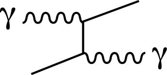
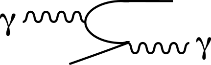
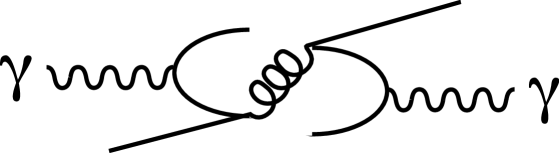
Figure 1: Photon-photon Interactions. (left) Direct interactions involve only electroweak couplings. (center) Once resolved process where one photon probes the parton structure of the other photon, similar to deep inelastic scattering. (right) Twice resolved process where the partons of each photon interact, similar to a $\rho-\rho$ collisions.

We use the Pythia pythiajetset Monte Carlo program to simulate the resolved photon cross sections, which are potential backgrounds to all other two-photon physics processes. These backgrounds, usually referred to as $\gamma\gamma\to{\rm hadrons}$, are also a concern at $e^{+}e^{-}$ and have been studied in detail teslagghh . However, at a $\gamma\gamma$ collider the high energy Compton photons provide an additional and dominant source of $\gamma\gamma\to{\rm hadron}$ background.

There has been a long standing discrepancy between the resolved photon backgrounds calculated by Pythia and those computed assuming the observed LEP cross section for $\gamma\gamma\rightarrow hadrons$ . This problem was mostly due to the parameters used by Pythia to describe this processes, and it is now understood. Nominally, we use the default settings for Pythia with the exception of the parameters listed in Table 1. The complete Pythia parameter list used is taken from Ref. jetweb . We find that $\sim 83\%$,$\sim 17\%$ and $\sim 0.4\%$ of interactions are due to photon-photon, photon-electron, and electron-electron interactions, respectively, and the photon-photon and photon-electron interaction cross section is dominated by resolved photons.

Table 1: Pythia parameter settings for resolved photon processes. Other parameters are taken from Ref. jetweb .

Parameter Setting	Explanation
MSTP(14)=30	Sets Structure of Photon
MSTP(53)=3	choice of pion parton distribution set
MSTP(54)=2	choice of pion parton distribution function library
MSTP(55)=N/A for MSTP(14)=30	choice of photon parton distribution set
MSTP(56)=2	choice of photon parton distribution function library
CKIN(3)=1.32	ptmin for hard $2\rightarrow$2 interactions

Over the energy range, $\sim 10-150$ GeV, of the LEP data the Pythia and LEP cross sections are in reasonable agreement, $\sim 400$ nb, as shown in Fig. 2. Also shown in Fig. 2 is the cross section for photon-electron processes, which are not negligible relative to the photon-photon processes. Beyond the range of the existing data, there are large uncertainties in the estimated of the once and twice resolved photon cross sections. These uncertainties at higher energies are a concern for a 500 GeV linear collider, but not for the lower energy Higgs factory. Ref. butterworthpaper provides an excellent discussion of the theoretical and experimental challenges of determining the photon structure. The most recent experimental data is from HERA hera and LEP-II lep . Despite the new data, there are large uncertaintes at small $x_{\gamma}$, and the uncertainties at large $x_{\gamma}$ are also significant. The QCD stucture function is probed by examining the high $E_{t}$ jets, but extrapolating to smaller $E_{t}$ introduces additional uncertainty. These large uncertainties could be reduce by data obtained from a proposed $\gamma\gamma$ engineering run at the SLC ourproposal .

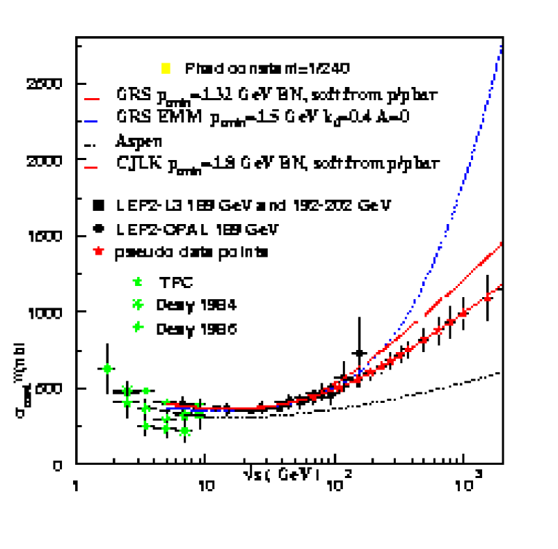
Figure 2: Photon-Photon and Photon-Electron Cross Section. (left) From Ref. albert . Updated photon-photon cross sections predicted by CJLK, GRS densities and measurements from LEP. (center) Photon-photon cross section and (right) Photon-electron cross section from Pythia using parameter described in the text.

Using these new sets of Pythia parameters, we can quatify the effect of this ‘extra’ beam related activity in the detector. For this purpose, we consider the beam parameters for $\sqrt{s}_{ee}=160$ GeV and $\sqrt{s}_{ee}=500$ GeV given in Table 2, and use the luminosity distributions shown in Fig. 3.

Table 2: Laser and electron beam parameters for ${\sqrt{s}}=160$ GeV ${\sqrt{s}}=500$ GeV. The beam parameters for ${\sqrt{s}}=500$ GeV differ from the NLC-$e^{+}e^{-}$ parameters. The bunch charge has been doubled to improve luminosity. Consequently, both the vertical emittance, $\epsilon_{y}$, and the bunch length, $\sigma_{z}$ are increased. Additionally, the total current is conserved as the rep. rate reduced by a factor of 2. The optimal laser wavelength decreases as the beam energy decreases. We assume that non-linear optics are used to triple the laser frequency for the ${\sqrt{s}}=160$ GeV machine and that this procedure is 70% efficient, thus more laser power is required.

Electron Beam Energy (GeV)	80	250
$\beta_{x}/\beta_{y}$ (mm)	1.4/0.08	4/0.065
$\epsilon_{x}/\epsilon_{y}~{}(\times 10^{-8})$	360/7.1	360/7.1
$\sigma_{x}/\sigma_{y}~{}({\rm nm})$	179/6	172/3.1
$\sigma_{z}$ (microns)	156	156
$N~{}(\times 10^{10})$	1.5	1.5
$e^{-}~{}{\rm Polarization}~{}(\%)$	80	80
rep. rate (Hz)	120$\times$95	120$\times$95
Laser Pulse Energy (J)	1.0/70%=1.4	1.0
Laser $\lambda$ (microns)	1.054/3 = 0.351	1.054
CP-IP distance (mm)	1	2

Figure 3: Luminosity for a $10^{7}$ sec year and associated expectation value for the product of photon polarizations, $\langle\lambda\lambda^{\prime}\rangle$, are plotted for $\sqrt{s}=160$ GeV ($x=4.1$ for $1.054/3~{}\mu$m laser wavelength), assuming 80% electron beam polarizations.

We process the events through the LC Fast MC detector simulation within the ROOTBrun:1997pa framework. The simulation includes calorimeter smearing and the detector configuration described in Section 4.1 of Chapter 15 of Ref. Abe:2001nr . From our preliminary studies, we find that the two-photon cross section is dominated by the twice resolved process at both 160 GeV and 500 GeV. For the beam parameters given in Table 2, we expect a background event rate of 6,700 and 20,500 events/second for the 160 GeV and 500 GeV machines, respectively. This corresponds to 0.6 and 1.8 overlay events per beam crossing. For the TBA machine beam parameters discussed in Ref.cliche , 0.1 overlay events per beam crossing are expected. Most of the products of the $\gamma\gamma\to$ hadrons will be produced at small angles relative to the photon beam and will escape undetected down the beam pipe. We are interested in the decay products that enter the detector. For this reason we are only considering tracks and showers with $|\cos\theta|<0.9$ in the laboratory frame, and we require tracks to have momentum greater than 200 MeV, while the showers must have energy greater than 100 MeV. The resulting track and shower energy distributions integrated over 17,000 beam crossings for $\sqrt{s}_{ee}=160$ GeV and 5,500 beam crossings for $\sqrt{s}_{ee}=500$ GeV are shown in Fig. 4-7, and summarized in Table 3. Experimental, theoretical and modeling errors have not yet been evaluated for these distributions.

Table 3: Event Multiplicity Due to Resolved Photon Backgrounds.

	160 GeV	500 GeV
Events/Crossing	0.6	1.8
Tracks/Crossing ($p>0.2$ GeV, $|\cos\theta|<0.9$)	3.7	14.6
Energy/Track ($p>0.2$ GeV, $|\cos\theta|<0.9$)	0.70 GeV	0.74 GeV
Clusters/Crossing ($E>0.1$ GeV, $|\cos\theta|<0.9$)	5.5	21.8
Energy/Cluster ($E>0.2$ GeV, $|\cos\theta|<0.9$)	0.45 GeV	0.49 GeV

Future studies of the physics possibilities of a $\gamma$C should include the impact of the resolved photons on the event reconstruction, and we need to determine the appropriate number of beam crossing that we need to integrate over. It is generally assumed that the $\gamma$C and $e^{+}e^{-}$ detectors will be the same or at least have comparable performance. At $e^{+}e^{-}$, the plan is to integrate over 100’s to 1000’s of beam crossings. This depends, of course, on the choice of detector technology as well as the bunch structure of the electron beam. At a $\gamma$C experiment, the desire to minimize the resolved photon backgrounds may drive the detector design to be able to minimize the number of crossings that are being readout together. In preliminary studies, integrating over about 10 crossings appears tractable. The required detector readout rate due to backgrounds from resolved photons call into question the assumptions that the $e^{+}e^{-}$ and $\gamma\gamma$ detectors will be based on the same technology and/or have comparable performance. An important distinction between the TESLA and NLC/TBA machine designs is the time between bunch crossings, 337 ns and $\leq$2.8 ns , respectively. The authors plan to study the difference between the detector design and performance.

The impact of resolved photon backgrounds on the physics reach of a $\gamma$C has yet to be determined. Previously, we reported that including the resolved photon contribution to the background in an analysis of $\gamma\gamma\to h\to\gamma\gamma$ korea cause a $S/B\sim 3$, and that the background was dominated by the resolved photons. However, now we know that the resolved photon background was overestimated by a factor of six.

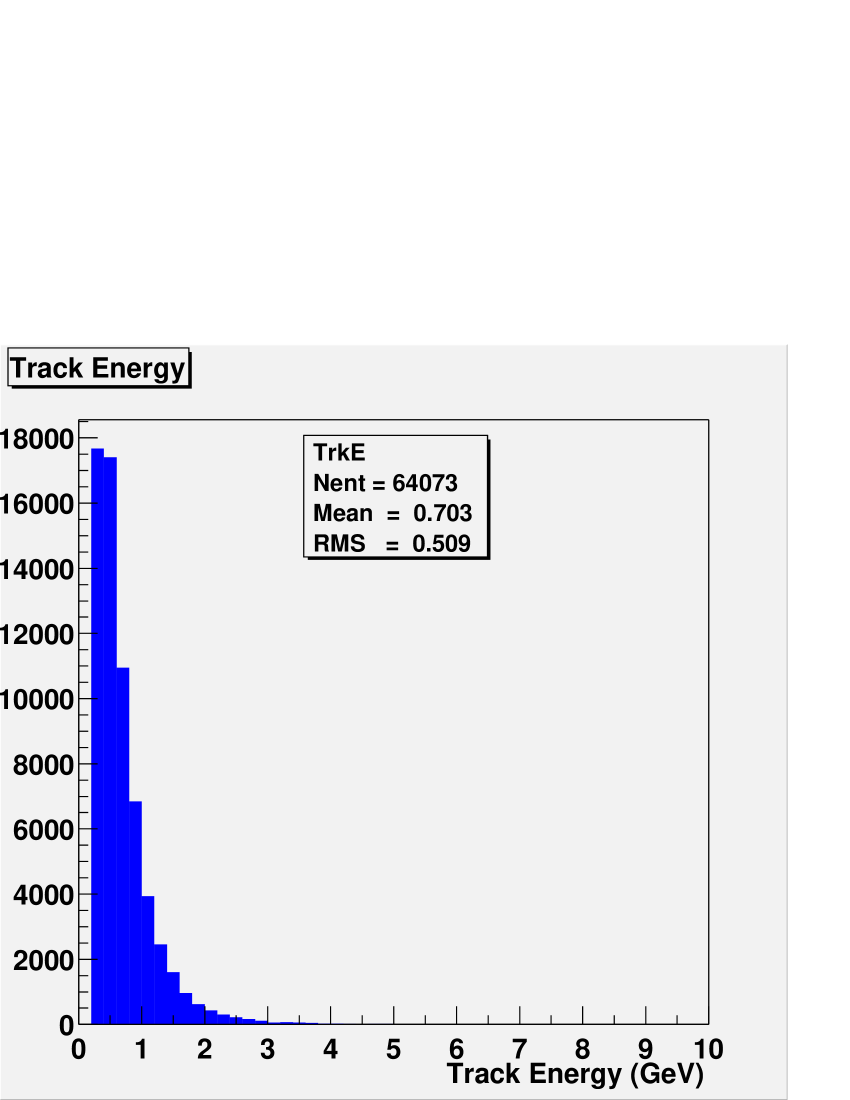
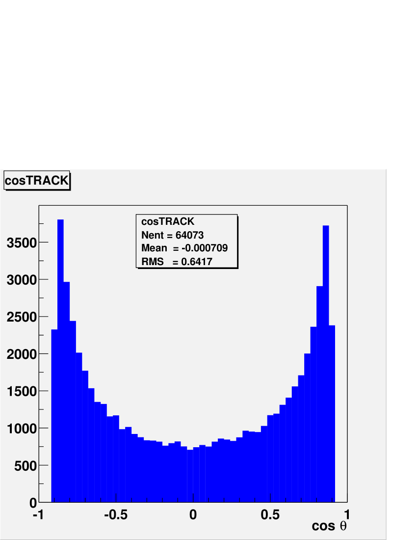
Figure 4: Tracks contributing to the resolved photon background for $\sqrt{s}_{ee}=160$ GeV. Energy and $\cos\theta$ distribution for tracks with $p>0.2$ GeV. The plots corresponds to 6,700 beam crossings.

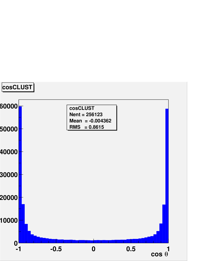
Figure 5: Showers contributing to the resolved photon background for $\sqrt{s}_{ee}=160$ GeV. Energy and $\cos\theta$ distribution for showers with $E>0.1$ GeV. The plots corresponds to 6,700 beam crossings.

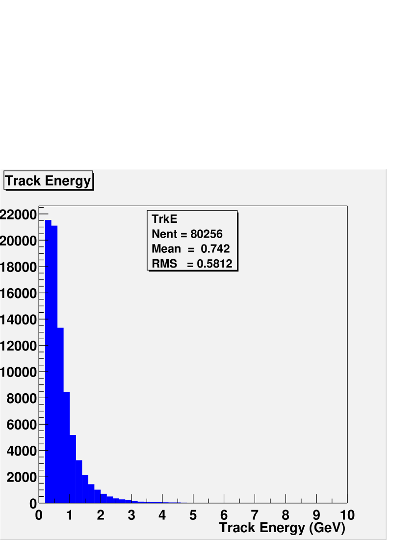
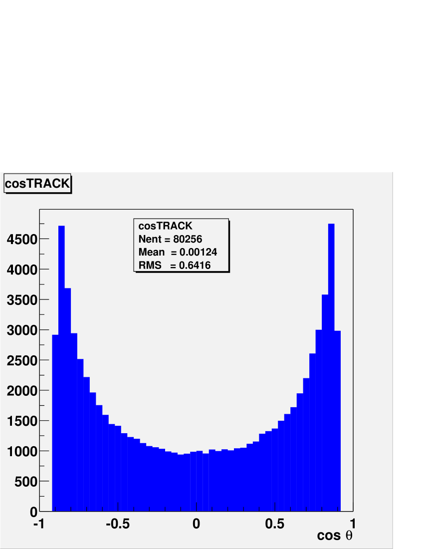
Figure 6: Tracks contributing to the resolved photon background for $\sqrt{s}_{ee}=500$ GeV. Energy and $\cos\theta$ distribution for tracks with $p>0.2$ GeV. The plots corresponds to 20,500 beam crossings.

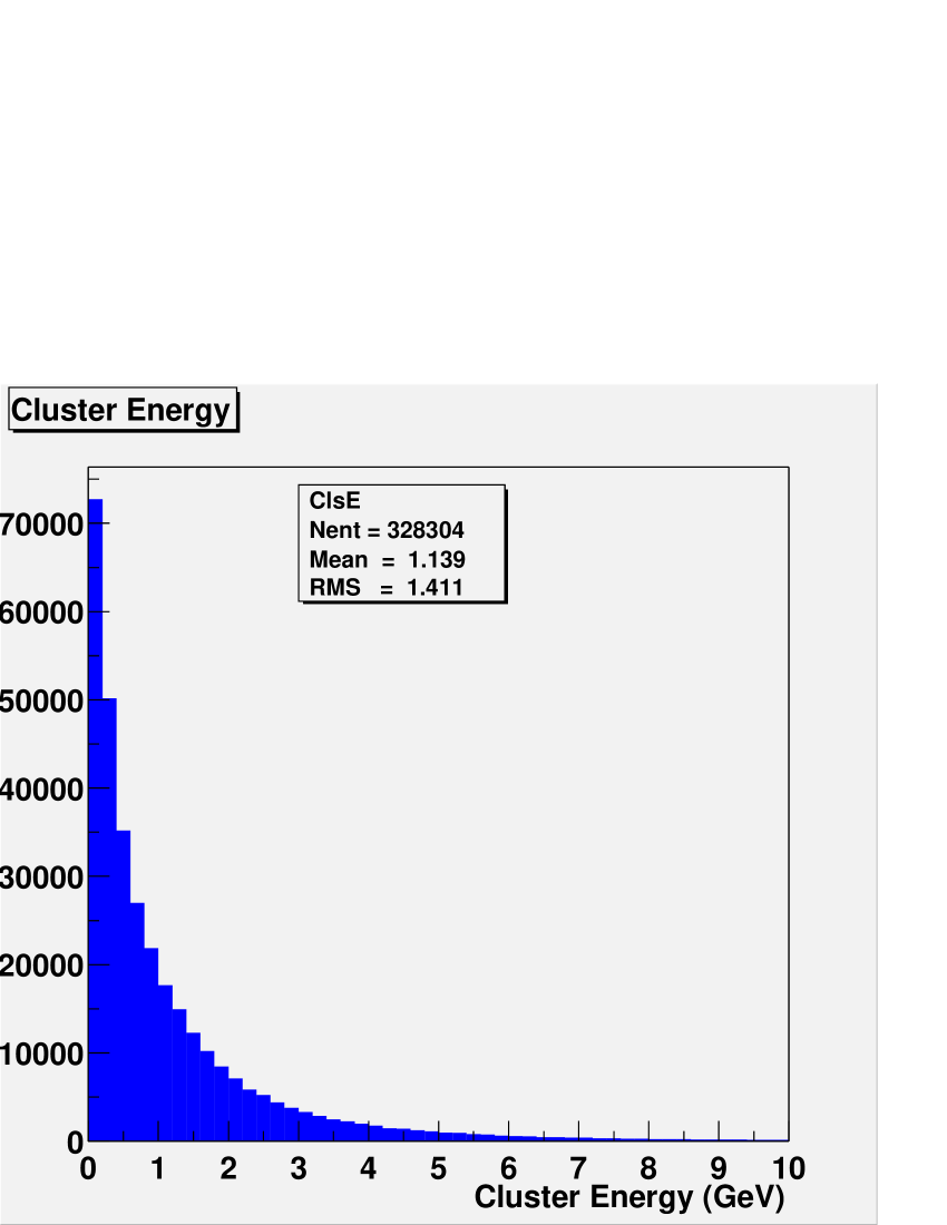
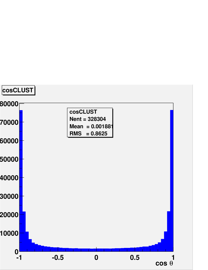
Figure 7: Showers contributing to the resolved photon background for $\sqrt{s}_{ee}=500$ GeV. Energy and $\cos\theta$ distribution for showers with $E>0.1$ GeV. The plots corresponds to 20,500 beam crossings.

III Physics studies

All the studies presented here are based on the CLICHE parameters given in cliche . This $\gamma$C was tunned for a 115 GeV Standard Model Higgs, and it is designed to be a Higgs factory capable of producing around 20,000 light Higgs bosons per year. The CLIC-1 beams and a laser backscattering system are expected to be capable of producing a $\gamma\gamma$ total (peak) luminosity of $2.0~{}(0.36)\times 10^{34}$ cm^-2s^-1, see Fig. 8. In the MSSM and some of the other models under consideration, the Higgs could have a mass as low as 90 GeV, and as high as 130 GeV. For the low mass case, the CLIC-1 energy could be lower, but an energy upgrade would be required in the high mass case.

Figure 8: Luminosity spectra and beam polarization as functions of $E_{CM}$($\gamma\gamma$) for the CLIC 1 parameters for 75 GeV electrons obtained with DIMAD dimad and CAIN cainref for ${{\cal L}_{ee}=4.8\times 10^{34}\rm cm^{-2}s^{-1}}$.

III.1 Standard Model expactations at the $\gamma$C Higgs factory

In the Standard Model, the branching ratios for ${\cal B}r(H\to b\bar{b})$, ${\cal B}r(H\to WW)$, ${\cal B}r(H\to ZZ)$ and ${\cal B}r(H\to\gamma\gamma)$ for a Higgs mass of 115 GeV are: 73.7%, 8.8% 0.9% and 0.2%, respectively. In cliche , it was shown that the most promising reaction for a 115 GeV Higgs, is $\gamma\gamma\rightarrow H\rightarrow{\bar{b}}b$, but the expectations for other decay channels like $H\rightarrow WW$ and $H\rightarrow\gamma\gamma$ were also given. Their results are summarized in Table 4.

However, since one of the objectives of a $\gamma$C Higgs factory would be to test the prediction for these branching ratios, and use their measurements to distinguish between the Standard Model and its possible extensions, we are making an effort to also look at the $\gamma\gamma\rightarrow H\rightarrow ZZ$. In order to evaluate the signal to background ratio in this decay mode, we need the cross sections for $\gamma\gamma\rightarrow ZZ$ and $\gamma\gamma\rightarrow four-fermions$.

We have made progress adding the processes $\gamma\gamma\rightarrow\gamma\gamma$, $\gamma\gamma\rightarrow ZZ$ and $\gamma\gamma\rightarrow\gamma Z$ to Pandora PeskinPandora . To date, these processes have not been included in Pandora as they are 1-loop processes, and as such the cross section is difficult to calculate. As it is the most interest to us, we have focused on the $\gamma\gamma\rightarrow ZZ$ process.

The FormCalc and LoopTools packages HahnLoopTools can be used to calculate the cross sections for various loop processes. We use code generated from these packages for us by Thomas Hahn, called AAAA, which can be used to calculate one loop integrals for general 2 to 2 processes, and 2 to 3 process. Given the mass, charge, polarization and nature (scalar, fermion, vector or photon) of the initial and final particles AAAA calculates the cross section for a given center of mass energy. We have modified the AAAA code to create a subroutine that returns the cross section for the process $\gamma\gamma\rightarrow ZZ$ given the masses of the $Z$’s, the initial and final polarizations, $\cos(\theta)$ and center of mass energy.

We have based the Pandora class for the $\gamma\gamma\rightarrow ZZ$ process on the $\gamma\gamma\rightarrow WW$ class. When the cross section is required by Pandora we call the subroutine discussed above.

The tools that we have develop will allows us to use the CAIN prediction of the full $\gamma\gamma$ energy spectra and their corresponding polarization. The expected cross section for $\gamma\gamma\rightarrow ZZ$ is smaller than 0.01 fb, for the CLICHE luminosity spectra and polarization shown in Fig. 8.

In order to determine the impact of $\gamma\gamma\rightarrow four-fermions$, background samples were generated with WHIZARD 1.24. For details concerning the usage of WHIZARD for four-fermion processes, please refer to point B3 below.

At the moment, we have only studied the prospects for the detection of $\gamma\gamma\rightarrow ZZ$ based on the search for the heaviest decay $b\bar{b}b\bar{b}$, and compare them to the light decays like $e^{+}e^{-}e^{+}e^{-}$, $e^{+}e^{-}\mu^{+}\mu^{-}$ and $\mu^{+}\mu^{-}\mu^{+}\mu^{-}$ final states.

The signal sample for $\gamma\gamma\rightarrow H\rightarrow ZZ\rightarrow b\bar{b}b\bar{b}$ was generated using Pythia 6.158 with an interface to CAIN to get the correct CLICHE spectrum. Event reconstruction and analysis were done in the framework of the FastMC program and PAW. About 75% of generated events had four or more reconstructed jets. We required $|cos\Theta_{j}|<0.9$ for $j=1,2,3,4$, where $\Theta_{j}$ is the polar angle of the jet with respect to the beam direction, measured in the lab frame. The efficiency of this cut for the four-fermion background processes depends strongly on the mass of the particle involved and for $\gamma\gamma\rightarrow b\bar{b}b\bar{b}$ it produces a 20-fold reduction of the initial sample. Meanwhile, signal events are distributed nearly isotropically, so that $\sim$70% of them will survive the cut.

Necessary signature to identify the $ZZ$ intermediate state is the appearance of the $Z$ mass peak. We therefore assume here that one $Z$ must be on the mass shell, leaving at most a 24 GeV mass for the other $Z$. Consequently, we selected only events for which one finds two jets with 85 GeV $<M_{j_{1}j_{2}}<$ 97 GeV, and the remaining two with 12 GeV $<M_{j_{3}j_{4}}<$ 30 GeV. It is to be noted that barely half of the Pythia-generated signal events do actually satisfy the above criteria. Final selection is done by looking at the four-jet invariant mass and taking events for which $M_{4j}>$ 100 GeV, which should include nearly all signal events which survived previous selection criteria. The final selection efficiency for signal events is around 25%.

No $b$ tagging was simulated. We assume an additioanl 70% efficiency for tagging a single $b\bar{b}$ pair. Taking $\sigma(\gamma\gamma\rightarrow H)$ = 112 fb, $BR(H\rightarrow ZZ)$ = 0.009 and $BR(Z\rightarrow b\bar{b})$ = 0.15, we end up at 0.6 reconstructed $\gamma\gamma\rightarrow H\rightarrow ZZ\rightarrow b\bar{b}b\bar{b}$ events per canonical year of $10^{7}s$. For the background, we have considered the direct $b\bar{b}b\bar{b}$ production, as well as $\gamma\gamma\rightarrow b\bar{b}c\bar{c}$ with a $c\bar{c}$ pair mistagged as $b\bar{b}$ and $\gamma\gamma\rightarrow c\bar{c}c\bar{c}$ with a double $c\bar{c}$ mistagging. We assume a 3.5% probability of mistagging $c\bar{c}$ as $b\bar{b}$. Total selection acceptance for background processes as a function of energy was found to vary from less than 0.01% for all three considered processes at 100 GeV and below to 0.4% at 120 GeV for $\gamma\gamma\rightarrow b\bar{b}b\bar{b}$, to 0.2% at 120 GeV for $\gamma\gamma\rightarrow b\bar{b}c\bar{c}$ and to 0.04% at 120 GeV for $\gamma\gamma\rightarrow c\bar{c}c\bar{c}$. Total cross sections in this energy region, calculated by WHIZARD 1.24, were found to be around 300 fb for $\gamma\gamma\rightarrow b\bar{b}b\bar{b}$, 8 pb for $\gamma\gamma\rightarrow b\bar{b}c\bar{c}$ and 90 pb for $\gamma\gamma\rightarrow c\bar{c}c\bar{c}$, and slowly varying with energy. From all this input, we arrive at a final number of 4.4 $b\bar{b}b\bar{b}$ events, 4.7 $b\bar{b}c\bar{c}$ events and 0.9 $c\bar{c}c\bar{c}$ events in the signal window per $10^{7}s$. Therefore, the signal to background is not optimal in this channel.

However, similar analysis for $Z\rightarrow ee,\mu\mu$ seem to give a better signal to background ratio, but higher monte carlo statistics is needed to be able to confirm. The reasons are the following: the reconstruction efficiency of the signal is much higher, and even though the $\sigma(\gamma\gamma\rightarrow 4l,l=e~{}or~{}\mu)$ are higher that for $b\bar{b}b\bar{b}$, their stronger $cos\Theta$ dependence causes most of the events to go down the beampipe. For example, $\sigma(\gamma\gamma\rightarrow 4\mu)$=0.16 nb, but only 1.7 fb have at least all four $\mu$’s in the detector.

Further work is needed before we can conclude, but the required tools are now available.

Table 4: The statistical errors on selected decay modes of a 115 GeV Higgs boson in the Standard Model. The $\gamma\gamma\to h$ cross section for the full (peak) ${\cal L_{\gamma\gamma}}$ is assumed to be 112 (624) fb (see Ref.cliche ). The expected yield for 200 (36) fb^-1 is 22,400 Higgs particles.

decay mode	raw events/year	S/B	$\epsilon_{sel}$	${\cal B}r$	$\Delta\Gamma_{\gamma\gamma}{\cal B}r/\Gamma_{\gamma\gamma}{\cal B}r$
${\bar{b}}b$	16509	2.0	0.20	73.7%	2%
$W^{+}W^{-}$	1971	1.2	0.32	8.8%	5%
$\gamma\gamma$	47	1.3	0.85	0.23%	22%
$ZZ$	201			0.9%	11%

III.2 NMSSM Scenario with $h\rightarrow aa$

In this section, we demonstrate that a $\gamma$C add-on to the CLIC test machines could provide invaluable complementarity to the LHC when it comes to studying and verifying difficult Higgs signals that can arise at the LHC in the context of the Next to Minimal Supersymmetric Model or other Higgs sectors in which a SM-like Higgs boson can decay to two lighter Higgs bosons.

III.2.1 Introduction

As repeatedly stressed, one of the key goals of the next generation of colliders is the discovery of Higgs boson(s) hhg . Assuming the absence of CP violation in the Higgs sector, the Higgs bosons of the Minimal Supersymmetric Model (MSSM) comprise the CP-even $h^{0}$ and $H^{0}$, the CP-odd $A^{0}$ and the charged Higgs, $H^{\pm}$. Recent reviews of the prospects for Higgs discovery and study at different colliders include Carena:2002es ; Gunion:2003fd . It has been established that the LHC with $L>100~{}{\rm fb}^{-1}$ will discover at least one of these Higgs bosons. A LC or a $\gamma$C will be able to perform detailed precision measurements of great importance to testing the details of the MSSM Higgs sector and are very likely to discover those Higgs bosons of the MSSM that can not be seen at the LHC. For example, the $\gamma$C can detect the $H^{0}$ and $A^{0}$ in the large-$m_{A^{0}}$, moderate-$\tan\beta$ wedge region where the LHC will not be able to detect them.

The results for the CP-conserving (CPC) MSSM do not generalize to supersymmetric models with more complicated Higgs sectors. One highly motivated extension of the MSSM is the Next-to-Minimal Supersymmetric Model (NMSSM), in which one additional singlet Higgs superfield is introduced in order to naturally explain the poorly understood $\mu$ parameter Ellis:1988er ; hhg . The NMSSM Higgs sector comprises three (mixed) CP-even states ($h_{1,2,3}$) two (mixed) CP-odd states ($a_{1,2}$) and a charged Higgs pair ($H^{\pm}$). Guaranteeing discovery of at least one NMSSM Higgs boson is a considerable challenge. In particular, one of the key ingredients in the no-lose theorem for CPC MSSM Higgs boson discovery is the fact that the SM-like Higgs boson (the $h$ when $m_{A}\mathrel{\raise 1.29167pt\hbox{$>$\kern-7.5pt\lower 4.30554pt\hbox{$\sim$}}}125~{}{\rm GeV}$ or $H$ when $m_{A}\mathrel{\raise 1.29167pt\hbox{$<$\kern-7.5pt\lower 4.30554pt\hbox{$\sim$}}}115~{}{\rm GeV}$) never has significant decays to other Higgs bosons ($h\to AA$ or $H\to AA,hh$, respectively). In the NMSSM, Higgs boson masses are not very strongly correlated, and $h_{1}\to a_{1}a_{1}$ or $h_{2}\to a_{1}a_{1}$ decays can be prominent Gunion:1996fb ; Dobrescu:2000jt . (If one-loop-induced CP violation is substantial in the MSSM Higgs sector, decays of one CP-mixed MSSM Higgs boson to two others are also possible Carena:2002bb .) Such decays fall outside the scope of the usual detection modes for the SM-like MSSM $h$ on which the MSSM no-lose LHC theorem largely relies. The first question is whether this makes an absolute LHC no-lose theorem for the NMSSM impossible. Second, if there are regions of parameter space in which the LHC signal is marginal or of uncertain interpretation, could a LC or (our particular interest here) a $\gamma$C  alone (i.e. in the absence of a LC) guarantee Higgs discovery or help verify the nature of the signal for such regions. The purpose of this note is to remark on the complementarity of a $\gamma$C to the LHC in such regions. We will find that it could be very crucial.

In earlier work Ellwanger:2001iw , a partial no-lose theorem for NMSSM Higgs boson discovery at the LHC was established. In particular, it was shown that the LHC would be able to detect at least one of the NMSSM Higgs bosons (typically, one of the lighter CP-even Higgs states) throughout the full parameter space of the model, excluding only those parameter choices for which there is sensitivity to the model-dependent decays of Higgs bosons to other Higgs bosons and/or superparticles.

In more recent work, the assumption of a heavy superparticle spectrum has been retained and the focus was on the question of whether or not this no-lose theorem can be extended to those regions of NMSSM parameter space for which Higgs bosons can decay to other Higgs bosons. It is found Ellwanger:2003jt that the parameter choices such that the “standard” discovery modes fail are such that either the $h_{1}$ or $h_{2}$ (numerically ordered according to increasing mass) is very SM-like in its couplings, but mainly decays to $a_{1}a_{1}$. Detection of $h_{1,2}\to a_{1}a_{1}$ will be difficult since each $a_{1}$ will decay primarily to either $b\overline{b}$ (or 2 jets if $m_{a_{1}}<2m_{b}$) and $\tau^{+}\tau^{-}$, yielding final states that will typically have large backgrounds at the LHC. In the end, there is a signal at the LHC for those cases in which the $a_{1}$ decays to $b\overline{b}$ with a substantial branching ratio even for these most difficult cases, but it will be hard to be sure if the signal really corresponds to a Higgs boson. We will show that a $\gamma$C  would be very important for clarifying the nature of the signal.

III.2.2 Details Regarding Earlier Results

In the earlier work, the simplest version of the NMSSM is considered, in which the term $\mu\widehat{H}_{1}\widehat{H}_{2}$ in the superpotential of the MSSM is replaced by (using the notation $\widehat{A}$ for the superfield and $A$ for its scalar component field)

$$\lambda\widehat{H}_{1}\widehat{H}_{2}\widehat{S}\ +\ \frac{\kappa}{3}\widehat{S}^{3}\ \ ,$$ (1)

so that the superpotential is scale invariant. No assumptions regarding the “universal” soft terms are made. Hence, the five soft supersymmetry breaking terms

$$m_{H_{1}}^{2}H_{1}^{2}\ +\ m_{H_{2}}^{2}H_{2}^{2}\ +\ m_{S}^{2}S^{2}\ +\ \lambda A_{\lambda}H_{1}H_{2}S\ +\ \frac{\kappa}{3}A_{\kappa}S^{3}$$ (2)

are considered as independent. The masses and/or couplings of sparticles are assumed to be such that their contributions to the loop diagrams for $gg\to h$ and $\gamma\gamma\to h$ couplings are negligible. In the stop sector, which appears in the radiative corrections to the Higgs potential, the soft masses $m_{Q}=m_{T}\equiv M_{susy}=1$ TeV are chosen. Scans are perfomred over the stop mixing parameter, related to $M_{susy}$ and the soft mixing parameter $A_{t}$ by $X_{t}\equiv 2\ \frac{A_{t}^{2}}{M_{susy}^{2}+m_{t}^{2}}\left(1-\frac{A_{t}^{2}}{12(M_{susy}^{2}+m_{t}^{2})}\right)\ .$ As in the MSSM, the value $X_{t}=\sqrt{6}$ – so called maximal mixing – maximizes the radiative corrections to the Higgs boson masses, and it is found that it leads to the most challenging points in NMSSM parameter space.

In the studies of Ellwanger:2003jt , a numerical scan over the free parameters is performed. For each point, the masses and mixings of the CP-even and CP-odd Higgs bosons, $h_{i}$ ($i=1,2,3$) and $a_{j}$ ($j=1,2$) are computed, taking into account radiative corrections up to the dominant two loop terms. Parameter choices excluded by LEP constraints on $e^{+}e^{-}\to Zh_{i}$ and $e^{+}e^{-}\to h_{i}a_{j}$ are eliminated and $m_{h^{\pm}}>155$ GeV is required, so that $t\to h^{\pm}b$ would not be seen. LHC discovery modes for a Higgs boson considered were (with $\ell=e,\mu$):

1) $gg\to h/a\to\gamma\gamma$;

2) associated $Wh/a$ or $t\bar{t}h/a$ production with $\gamma\gamma\ell^{\pm}$ in the final state;

3) associated $t\bar{t}h/a$ production with $h/a\to b\bar{b}$;

4) associated $b\bar{b}h/a$ production with $h/a\to\tau^{+}\tau^{-}$;

5) $gg\to h\to ZZ^{(*)}\to$ 4 leptons;

6) $gg\to h\to WW^{(*)}\to\ell^{+}\ell^{-}\nu\bar{\nu}$;

7) $WW\to h\to\tau^{+}\tau^{-}$;

8) $WW\to h\to WW^{(*)}$.

The expected statistical significances at the LHC in all Higgs boson detection modes 1) – 8) was estimated by rescaling results for the SM Higgs boson and/or the the MSSM $h,H$ and/or $A$. Among these modes, the $t\overline{t}h\to t\overline{t}b\overline{b}$ mode is quite important. The experimentalists extrapolated this beyond the usual SM mass range of interest. Results for $N_{SD}=S/\sqrt{B}$ (where $S$ and $B$ are the signal and background, respectively) assuming $K_{S}=K_{B}=1$ were employed, awaiting the time when all $K$ factors are known. (For all cases where both $K_{S}$ and $K_{B}$ are known, their inclusion improves the $N_{SD}$ value.) For each mode, the procedure was to use the results for the “best detector” (e.g. CMS for the $t\overline{t}h$ channel), assuming $L=300~{}{\rm fb}^{-1}$ for that one detector.

Some things that changed between the 1st study of Ellwanger:2001iw and the 2nd study of Ellwanger:2003jt were the following. 1) The $gg\to h_{SM}\to\gamma\gamma$ $N_{SD}$ values from CMS were reduced by the inclusion of detector cracks and other such detector details. 2) The CMS $t\overline{t}h_{SM}\to t\overline{t}b\overline{b}$ $N_{SD}$ vales came in substantially larger than the ATLAS values. 3) The experimental evaluations of the $WW$ fusion channels yield lower $N_{SD}$ values than the original theoretical estimates.

The results from Ellwanger:2001iw can be summarized as follows. For parameter space regions where none of the “higgs-to-higgs” decays

$$i)\ h\to h^{\prime}h^{\prime}\;,\quad ii)\ h\to aa\;,\quad iii)\ h\to h^{\pm}h^{\mp}\;,\quad iv)\ h\to aZ\;,$$

$$v)\ h\to h^{\pm}W^{\mp}\;,\quad vi)\ a^{\prime}\to ha\;,\quad vii)\ a\to hZ\;,\quad viii)\ a\to h^{\pm}W^{\mp}\;.$$

is kinematically allowed it is possible for the LHC signals to be much weaker than SM Higgs signals. In particular, one can find parameters such that the $gg\to h_{i}\to\gamma\gamma$ rates are all greatly suppressed and all the $h_{i}\to WW$ branching fractions and couplings are suppressed. The result is greatly decreased $N_{SD}$ values for all the channels 1) – 8), and a not very wonderful combined statistical significance after summing over various sets of channels. Nonetheless, the very worst parameter choices for the no-higgs-to-higgs decay part of parameter space does predict a $\geq 5\sigma$ signal for at least one Higgs boson in at least one channel — in particular, in the $t\overline{t}h\to t\overline{t}b\overline{b}$ channel or the $WW\to h\to\tau^{+}\tau^{-}$ channel.

In order to probe the complementary part of the parameter space, in Ellwanger:2003jt , it was required that at least one of the decay modes $i)-viii)$ is allowed. In the set of randomly scanned points, those for which all the statistical significances in modes 1) – 8) are below $5\sigma$ were selected. There were a lot of points, all with similar characteristics. Namely, in the Higgs spectrum, there is a very SM-like CP-even Higgs boson with a mass between 115 and 135 GeV (i.e. above the LEP limit), which can be either $h_{1}$ or $h_{2}$, with essentially full strength coupling to the gauge bosons. This state decays dominantly to a pair of (very) light CP-odd states, $a_{1}a_{1}$, with $m_{a_{1}}$ between 5 and 65 GeV. (The singlet component of $a_{1}$ has to be small in order to have a large $h_{1}\to a_{1}a_{1}$ or $h_{2}\to a_{1}a_{1}$ branching ratio when the $h_{1}$ or $h_{2}$, respectively, is the SM-like Higgs boson.) Since the $h_{1}$ or $h_{2}$ is very SM-like, the $e^{+}e^{-}\to h_{1}a_{1}$ or $e^{+}e^{-}\to h_{2}a_{1}$ associated production processes have very low rate and place no constraint on the light CP-odd state at LEP. For illustration, six difficult benchmark points were selected. The features of these points are displayed in Table 5. For points 1 – 3, $h_{1}$ is the SM-like CP-even state, while for points 4 – 6 it is $h_{2}$. One should note the large $BR(h\to a_{1}a_{1})$ of the SM-like $h$ ($h=h_{1}$ for points 1 – 3 and $h=h_{2}$ for points 4 –6). For points 4 – 6, with $m_{h_{1}}<100~{}{\rm GeV}$, the $h_{1}$ is mainly singlet and therefore evades LEP constraints. Further, in the case of the points 1 – 3, the $h_{2}$ would not be detectable either at the LHC or the LC. For points 4 – 6, the $h_{1}$, though light, is singlet in nature and would not be detectable. Further, the $h_{3}$ or $a_{2}$ will only be detectable for points 1 – 6 if a super high energy LC is eventually built so that $e^{+}e^{-}\to Z\to h_{3}a_{2}$ is possible. Thus, it was necessary to focus on searching for the SM-like $h_{1}$ ($h_{2}$) for points 1 – 3 (4 – 6) using the dominant $h_{1}(h_{2})\to a_{1}a_{1}$ decay mode.

Table 5: Properties of selected scenarios that could escape detection at the LHC. The production rate for $gg\to h_{i}$ fusion relative to the $gg$ fusion rate for a SM Higgs boson with the same mass is given. Important absolute branching ratios are displayed. For points 2 and 6, $BR(a_{1}\to jj)\simeq 1-BR(a_{1}\to\tau^{+}\tau^{-})$. For the heavy $h_{3}$ and $a_{2}$, only their masses are shown. For all points 1 – 6, the statistical significances for the detection of any Higgs boson in any of the channels 1) – 8) (as listed in the introduction) are tiny; their maximum is indicated in the last row, together with the process number and the corresponding Higgs state.

Point Number	1	2	3	4	5	6
Bare Parameters
$\lambda$	0.2872	0.2124	0.3373	0.3340	0.4744	0.5212
$\kappa$	0.5332	0.5647	0.5204	0.0574	0.0844	0.0010
$\tan\beta$	2.5	3.5	5.5	2.5	2.5	2.5
$\mu_{\rm eff}~{}({\rm GeV})$	200	200	200	200	200	200
$A_{\lambda}~{}({\rm GeV})$	100	0	50	500	500	500
$A_{\kappa}~{}({\rm GeV})$	0	0	0	0	0	0
CP-even Higgs Boson Masses and Couplings
$m_{h_{1}}$ (GeV)	115	119	123	76	85	51
Relative gg Production Rate	0.97	0.99	0.99	0.00	0.01	0.08
$BR(h_{1}\to b\overline{b})$	0.02	0.01	0.01	0.91	0.91	0.00
$BR(h_{1}\to\tau^{+}\tau^{-})$	0.00	0.00	0.00	0.08	0.08	0.00
$BR(h_{1}\to a_{1}a_{1})$	0.98	0.99	0.98	0.00	0.00	1.00
$m_{h_{2}}$ (GeV)	516	626	594	118	124	130
Relative gg Production Rate	0.18	0.09	0.01	0.98	0.99	0.90
$BR(h_{2}\to b\overline{b})$	0.01	0.04	0.04	0.02	0.01	0.00
$BR(h_{2}\to\tau^{+}\tau^{-})$	0.00	0.01	0.00	0.00	0.00	0.00
$BR(h_{2}\to a_{1}a_{1})$	0.04	0.02	0.83	0.97	0.98	0.96
$m_{h_{3}}$ (GeV)	745	1064	653	553	554	535
CP-odd Higgs Boson Masses and Couplings
$m_{a_{1}}$ (GeV)	56	7	35	41	59	7
Relative gg Production Rate	0.01	0.03	0.05	0.01	0.01	0.05
$BR(a_{1}\to b\overline{b})$	0.92	0.00	0.93	0.92	0.92	0.00
$BR(a_{1}\to\tau^{+}\tau^{-})$	0.08	0.94	0.07	0.07	0.08	0.90
$m_{a_{2}}$ (GeV)	528	639	643	560	563	547
Charged Higgs Mass (GeV)	528	640	643	561	559	539
Most Visible Process No.	2 ($h_{1}$)	2 ($h_{1}$)	8 ($h_{1}$)	2 ($h_{2}$)	8 ($h_{2}$)	8 ($h_{2}$)
Significance at 300 ${\rm fb}^{-1}$	0.48	0.26	0.55	0.62	0.53	0.16

LHC, $\sqrt{s_{pp}}=14$ TeV

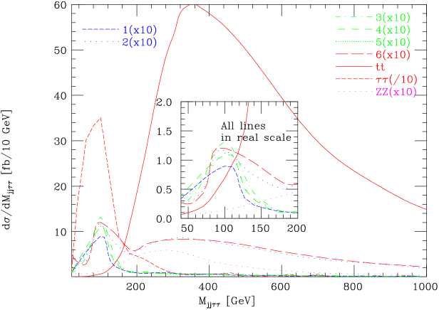
Figure 9: Reconstructed mass of the $jj\tau^{+}\tau^{-}$ system for signals and backgrounds after the selections described, at the LHC. The distribution $d\sigma/dM_{jj\tau^{+}\tau^{-}}$ [fb/10 GeV] vs. $M_{jj\tau^{+}\tau^{-}}$ [GeV] is plotted. The lines corresponding to points 4 and 5 are visually indistinguishable. No $K$ factors are included.

For points 1 and 3 – 5, $a_{1}\to b\overline{b}$ decays are dominant with $a_{1}\to\tau^{+}\tau^{-}$ making up the rest. In the case of points 2 and 6, $m_{a_{1}}<2m_{b}$ so that $a_{1}\to\tau^{+}\tau^{-}$ decays are dominant, with $a_{1}\to jj$ decays making up most of the rest. For points 1 and 3 – 5, the $b$ jets will not be that energetic and $b$-tagging will be somewhat inefficient. However, because of a large $jj\tau^{+}\tau^{-}$ background from Drell-Yan $\tau^{+}\tau^{-}$ pair production, $b$-tagging will be needed. The situation is illustrated in Fig. 9, where the cross section vs. the reconstructed $M_{jj\tau^{+}\tau^{-}}$ is plotted. The signals and backgrounds are plotted prior to the implementation of $b$-tagging. For all six NMSSM setups, the Higgs resonance produces a somewhat amorphous bump in the very end of the low mass tail of the $t\bar{t}$ background (see the insert in the top frame of Fig. 9). The large size of the $\tau^{+}\tau^{-}$ background is apparent. After implementing single $b$-tagging, assuming criteria for which $\epsilon_{b}=0.5$ and $\epsilon_{mis-tag}=0.01$, the signal and $t\overline{t}$ background rates will be reduced by a factor of about 2 and the $\tau$ background will be negligible for points 1 and 3 – 5. (Viable techniques for observation of points 2 and 6 have not yet been developed.) Although the signal is somewhat amorphous in nature, statistics are significant. To estimate $S/\sqrt{B}$, the following procedure was employed. First, assume $L=300~{}{\rm fb}^{-1}$, a $K$ factor of 1.1 for $WW$ fusion and a $K$ factor of 1.6 for the $t\overline{t}$ background. (These $K$ factors are not included in the plots of Fig. 9.) Then, sum events over the region $60\leq M_{jj\tau^{+}\tau^{-}}\leq 90$ GeV. Assuming a net efficiency of 50% for single $b$-tagging, the $t\overline{t}$ background rate is $B\sim 160$. For points 1 and 3 – 5, one finds signal rates of about $S=445$, $375$, $515$, $460$, corresponding to $N_{SD}=S/\sqrt{B}$ of 35, 30, 41 and 36, respectively. However, given the broad distribution of the signal, it is clear that a crucial question will be the accuracy with which the background shape can be predicted from theory. (The background normalization after the cuts imposed in the analysis would be very well known from the higher $M_{jj\tau^{+}\tau^{-}}$ regions.) Even more important is the question of how certain the interpretation of this signal will be, given that it would be the only signal for Higgs boson production. In this regard, detection of the $a_{1}a_{1}\to b\overline{b}b\overline{b}$ final state would be very valuable as it would allow us to determine if $BR(a_{1}\to\tau^{+}\tau^{-})/BR(a_{1}\to b\overline{b})$ was in the ratio predicted (by the ratio of fermion masses). However, there are large backgrounds in the $b\overline{b}b\overline{b}$ final state. A study is in progress.

III.2.3 The role of a $\gamma$C

While further examination of and refinements in the LHC analysis may ultimately lead one to have good confidence in the viability of the NMSSM Higgs boson signals discussed above, an enhancement at low $M_{jj\tau^{+}\tau^{-}}$ of the type shown (for some choice of $m_{a_{1}}$) will nonetheless be the only evidence on which a claim of LHC observation of Higgs bosons can be based. Ultimately, confirmation and further study at another collider will be critical.

One possibility would be an LC, with energy up to 800 GeV. (In the following, $h=h_{1}$ for points 1–3 and $h=h_{2}$ for points 4–6 in Table 5.) Because the $ZZh$ coupling is nearly full strength in all cases, and because the $h$ mass is of order 100 GeV, discovery of the $h$ would be very straightforward via $e^{+}e^{-}\to Zh$ using the $e^{+}e^{-}\to ZX$ reconstructed $M_{X}$ technique which is independent of the “unexpected” complexity of the $h$ decay to $a_{1}a_{1}$. This would immediately provide a direct measurement of the $ZZh$ coupling with very small error. The next stage would be to look at rates for the various $h$ decay final states, $F$, and extract $BR(h\to F)=\sigma(e^{+}e^{-}\to Zh\to ZF)/\sigma(e^{+}e^{-}\to Zh)$. For the NMSSM points considered here, the main channels would be $F=b\overline{b}b\overline{b}$, $F=b\overline{b}\tau^{+}\tau^{-}$ and $F=\tau^{+}\tau^{-}\tau^{+}\tau^{-}$. At the LC, a fairly accurate determination of $BR(h\to F)$ should be possible in all three cases. This would allow us to determine $BR(h\to a_{1}a_{1})$ independently. As demonstrated in Ellwanger:2003jt , the $WW$ fusion production mode would also yield an excellent signal and provide a second means for studying the $h$ and its decays. Indeed, at 800 GeV or above, $WW$ fusion is the dominant Higgs boson production channel for CP-even Higgs bosons in the intermediate mass range.

Here, however, we wish to focus on the $\gamma$C. In scenarios (1), (3), (4) and (5) outlined in Table 6, the main signal channel to look for experimentally is $\gamma\gamma\rightarrow h\rightarrow aa\rightarrow b\bar{b}b\bar{b}$. A sizable signal would also be present for the $b\bar{b}\tau^{+}\tau^{-}$ final state. In scenarios (2) and (6), the most promising channel to look at is $\gamma\gamma\rightarrow h\rightarrow aa\rightarrow\tau^{+}\tau^{-}\tau^{+}\tau^{-}$. In what follows, we will demonstrate the photon collider potential for observing the $h_{NMSSM}\rightarrow aa$ decay based on the detection of its $b\bar{b}b\bar{b}$ final state.

Samples of signal and background events were generated and respective detector responses simulated. Signal samples were generated with Pythia 6.158, using a full $\gamma\gamma$ luminosity spectrum as obtained from CAIN. We assume here the standard CLICHE spectrum as employed in cliche , which peaks at $E_{CM}=115$ GeV and falls off quickly at larger energies. Note that in most scenarios under consideration here, $m_{h}>115$ GeV, and so this particular spectrum is unlikely to be the optimum in the general case. The Pythia process $\gamma\gamma\rightarrow H\rightarrow AA$ was considered, where $H$ and $A$ are usually taken to be the “heavy” scalar and pseudoscalar Higgs bosons, respectively (e.g., in the MSSM). Their masses were set accordingly to the respective $h$ and $a$ masses in the four relevant NMSSM scenarios. The $H$ couplings were changed by hand to ensure a close to unity branching fraction for $H\rightarrow AA$. Overall normalization was given by the total cross section for $\gamma\gamma\rightarrow h_{SM}$, where $h_{SM}$ is the Standard Model Higgs boson of an appropriate mass. Higgs production cross sections in each of the four relevant scenarios are listed in Table 6 (fourth column).

The main background sources are the direct four-quark production processes: $\gamma\gamma\rightarrow b\bar{b}b\bar{b}$, $\gamma\gamma\rightarrow b\bar{b}c\bar{c}$ with a $c\bar{c}$ pair mistagged as $b\bar{b}$, and $\gamma\gamma\rightarrow c\bar{c}c\bar{c}$ with a double $c\bar{c}$ mistagging. Background samples were generated with WHIZARD 1.24. Several cross checks of WHIZARD have been done, which are relevant for this analysis. The four-fermion generator in WHIZARD was cross checked for the processes $\gamma\gamma\rightarrow e^{+}e^{-}e^{+}e^{-}$, $e^{+}e^{-}\mu^{+}\mu^{-}$ and $\mu^{+}\mu^{-}\mu^{+}\mu^{-}$, and output cross sections were found to be consistent with existing theoretical computations 4lept . Typical cross sections in this energy region were found to be around 300 fb for $\gamma\gamma\rightarrow b\bar{b}b\bar{b}$, 8 pb for $\gamma\gamma\rightarrow b\bar{b}c\bar{c}$ and 90 pb for $\gamma\gamma\rightarrow c\bar{c}c\bar{c}$, and slowly varying with energy. The effects of beam polarization were cross checked between WHIZARD and Pythia for $\gamma\gamma\rightarrow b\bar{b}$ and $c\bar{c}$ and found to be consistent. For the four fermion processes, beam polarization plays a minor role. Events were generated at several fixed center-of-mass energies, analysis was consistently repeated for every sample. Correct $\gamma\gamma$ luminosity spectra were obtained by interpolation of the results (cross sections and selection efficiencies) to arbitrary intermediate energies and applying appropriate weights to events.

Event reconstruction and analysis was done in the framework of the FastMC program. We required exactly 4 reconstructed jets and $|cos\Theta_{j}|<0.9$ for $j=1,2,3,4$, where $\Theta_{j}$ is the polar angle of the jet with respect to the beam direction, measured in the lab frame. Four-fermion processes have angular distributions strongly peaked at small angles, so that this cut reduces the amount of surviving background by up to two orders of magnitude. Meanwhile, signal events are distributed nearly isotropically, with $\sim$80% of them surviving the cut.

The remaining events were checked for the two-jet invariant masses. From the three possible combinations of two two-jet invariant masses in a four-jet event, the one yielding two values the closest to each other was selected. We required consistency of the two values within 10 GeV. The acceptance of this cut is close to 100% for signal events and around 60% for background events.

No $b$ tagging was simulated. We assume a 50% $b$ tagging efficiency and a 3.5% probability of mistagging a $c\bar{c}$ pair as $b\bar{b}$.

Table 6: NMSSM points 1,3,4,5. We give cross sections, acceptance after all cuts other than $b$-tagging, and the number of events (assuming a $b$-tagging efficiency of $\epsilon_{b}=0.5$) in a canonical $10^{6}$ second year.

Scenario	$m_{h}$ (GeV)	$m_{a}$ (GeV)	$\sigma(\gamma\gamma\rightarrow h)$ (fb)	Acceptance	No. events / 10${}^{6}s$
(1)	115	56	112	0.26	139
(3)	123	35	9.1	0.33	14.7
(4)	118	41	46	0.28	63
(5)	124	59	6.0	0.24	7.1

Signal samples remaining at this point in each of the four scenarios considered, normalized to $10^{6}s$ of data taking, are given in Table 6 (quoted acceptances do not include the $b$ tagging efficiency). Obviously, the final amount of signal strongly depends on the $h$ mass. This dependence is, however, almost entirely due to the luminosity spectrum assumed and the resulting sensitivity of the total $h$ production cross section to $m_{h}$.

The expected four-jet invariant mass distributions of all surviving signal and background events are depicted in Fig. 10 (the background samples are the same in each case). Absolute numbers are again normalized to $10^{6}$ seconds. We find a clear signal, visible over the background after a short time of running, even in the most disfavorable scenario (5). It is also clear that the particular choice of $E_{CM}=115$ GeV was not the most fortunate for this study and that an upgrade of $E_{CM}$ to 120-125 GeV would very probably have the effect of producing signals for cases (3) and (5) that look much more like those shown here for cases (1) and (4). If the beam energy happens to be well tuned to $m_{h}$ (as was the case here for scenario (1)), a prominent signal peak in the four-jet invariant mass is bound to appear immediately.

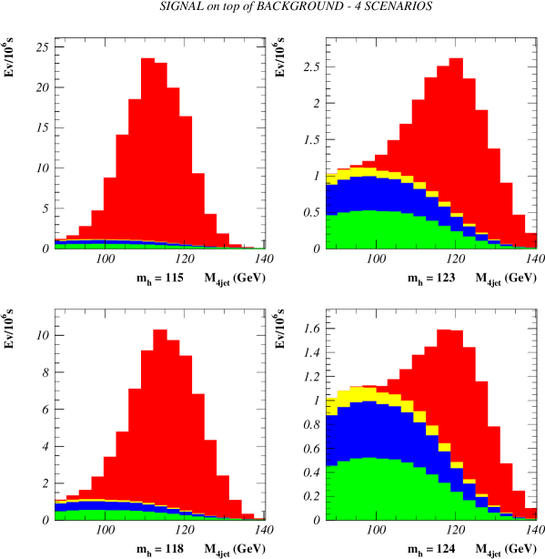
Figure 10: Four-jet invariant mass distributions after $10^{6}s$ of running, and after including $b$-tagging with $\epsilon_{b}=0.5$, in scenarios (1), (3), (4) and (5). Signal $\gamma\gamma\rightarrow h\rightarrow aa\rightarrow b\bar{b}b\bar{b}$ is shown in red, backgrounds: $\gamma\gamma\rightarrow b\bar{b}b\bar{b}$ in green, $\gamma\gamma\rightarrow b\bar{b}c\bar{c}$ in blue and $\gamma\gamma\rightarrow c\bar{c}c\bar{c}$ in yellow.

For the two scenarios not considered here, (2) and (6), the prospects for observing $\gamma\gamma\rightarrow h\rightarrow aa\rightarrow\tau^{+}\tau^{-}\tau^{+}\tau^{-}$ are potentially just as good as found here for the $b\overline{b}b\overline{b}$ channel for scenarios (1) and (3 – 5). With the cross section for direct 4$\tau$ production being of the order of 500 fb, the final signal to background ratio should, in fact, be very similar to the one obtained here in the 4$b$ channel, except for the slightly different $h$ masses; the overall normalization will depend on the $\tau$ reconstruction efficiency. The main difficulty will be the impossibility of fully reconstructing the mass peak in the $\tau^{+}\tau^{-}\tau^{+}\tau^{-}$ channel. A full study is needed.

Returning to scenarios (1), (3), (4) and (5) given Table 6, we note that $BR(a\rightarrow\tau^{+}\tau^{-})\approx 0.1$ so that signal detection seems plausible also in the channel $b\bar{b}\tau^{+}\tau^{-}$, provided $m_{h}$ is not too far away from $E_{CM}$ (a slight upgrade of $E_{CM}$ should be enough for this purpose). Combination of data obtained from the two channels will provide invaluable information for physics studies. In particular, the very important ratio $BR(a_{1}\to\tau^{+}\tau^{-})/BR(a_{1}\to b\overline{b})$ can be measured and the consistency with predictions for this ratio in the case of the NMSSM (or more generally with expectations for a pseudoscalar Higgs boson) can be checked. In addition, we can expect that other possible decay modes for the $h$ can be strictly limited, allowing a determination of the absolute rate for $\gamma\gamma\to h$ production and hence of $\Gamma(h\to\gamma\gamma)$. The magnitude of this partial width is determined primarily by the $h$’s couplings to $WW$, $t\overline{t}$ and $b\overline{b}$ (assuming a heavy sparticle spectrum in the case of the NMSSM). Thus, a measurement of $\Gamma(h\to\gamma\gamma)$ provides invaluable constraints on these couplings and would, in particular, allow us to check for consistency with their being approximately SM-like.

III.2.4 Conclusions for the NMSSM

We have demonstrated that a $\gamma$C would provide an invaluable confirmation of the very amorphous and difficult to interpret LHC signals for $h\to aa$ production that would be present in the $aa\to b\overline{b}\tau^{+}\tau^{-}$ channel. In particular, we have demonstrated a clear signal in the important complementary channel $aa\to b\overline{b}b\overline{b}$. We have also argued that the other two final state channels of $aa\to b\overline{b}\tau^{+}\tau^{-}$ and $aa\to\tau^{+}\tau^{-}\tau^{+}\tau^{-}$ will also yield clear signals at a $\gamma$C that will allow us to confirm the Higgs boson nature of the signals. In contrast, the viability of a LHC signal in the $aa\to b\overline{b}b\overline{b}$ final state is quite uncertain. Finally, in cases where $m_{a}$ is so small that $a\to b\overline{b}$ decays are not allowed, we believe that the $\gamma$C will be able to detect the $aa\to\tau^{+}\tau^{-}\tau^{+}\tau^{-}$ and possibly the $aa\to jj\tau^{+}\tau^{-}$ final states that have not yet been shown to be detectable at the LHC.

III.3 Higgs boson physics in the Complex MSSM

The MSSM with complex parameters (cMSSM) offers an interesting extension of the “real MSSM” (rMSSM), especially concerning Higgs boson physics. At the tree-level, ${\cal CP}$-violation in the Higgs boson sector is absent. However, complex phases of the trilinear couplings, $A_{t}$, $A_{b}$, …, of the gluino mass and of the gaugino masses, $m_{\widetilde{g}}$, $M_{2}$ and $M_{1}$ and possibly also from the Higgs mixing parameter $\mu$ can induce ${\cal CP}$-violation at the loop-level. As a consequence all three neutral Higgs bosons, $h$, $H$ and $A$ are no longer ${\cal CP}$ eigenstates, but can mix with each other mhiggsCPXgen ,

$$\left(h,H,A\right)\to\left(h_{1},h_{2},h_{3}\right){\rm~{}~{}~{}with~{}~{}}m_{h_{1}}\leq m_{h_{2}}\leq m_{h_{3}}~{}.$$ (3)

Higher order corrections to the Higgs boson masses and couplings have been evaluated in several approaches mhiggsCPXEP ; mhiggsCPXRG1 ; mhiggsCPXRG2 ; mhiggsCPXFD1 .

Due to loop corrections, the lightest Higgs boson can decouple from the gauge bosons. In this case, at $e^{+}e^{-}$ colliders, the main production modes for Higgs bosons can be

$$e^{+}e^{-} \to Z\,\to\,Z\,h_{2}$$

$$e^{+}e^{-} \to Z\,\to\,h_{2}\,h_{1}~{}.$$ (4)

Higgs boson searches at LEP in the context of the cMSSM mhexpOPAL have shown that in this case the decay $h_{2}\to h_{1}h_{1}$ poses special experimental problems. This decay mode, which is often dominant in this case, results in a six jet final state topology (with the Higgs bosons decaying to $b$ quarks). Such a final state can be quite complicated to handle, e.g. due to jet pairing problems.

In a $\gamma$C the situation is more favorable. Here the Higgs bosons are produced singly. Thus the decay $h_{2}\to h_{1}h_{1}$ results in a four jet final state that is easy to handle. (In a similar fashion the problem at an $e^{+}e^{-}$ collider could be overcome if the Higgs bosons are produced in the $WW$ fusion mode at high energies.) The topology of the decay $h_{2}\to h_{1}h_{1}$ resembles strongly the topology that arises for $h\to AA$ in the rMSSM, the NMSSM or the THDM. Thus the analysis methods can (nearly) directly be taken over from these cases.

III.4 The Little Higgs boson at a Photon Collider

The Standard Model (SM) of the strong and electroweak interactions has passed stringent tests up to the highest energies accessible today. The precision electroweak data Hagiwara:fs point to the existence of a light Higgs boson in the SM, with mass $m_{H}\mathrel{\raise 1.29167pt\hbox{$<$\kern-7.5pt\lower 4.30554pt\hbox{$\sim$}}}200$ GeV. The Standard Model with such a light Higgs boson can be viewed as an effective theory valid up to a much higher energy scale $\Lambda$, possibly all the way up to the Planck scale. In particular, the precision electroweak data exclude the presence of dimension-six operators arising from strongly coupled new physics below a scale $\Lambda$ of order 10 TeV Barbieri ; if new physics is to appear below this scale, it must be weakly coupled. However, without protection by a symmetry, the Higgs mass is quadratically sensitive to the cutoff scale $\Lambda$ via quantum corrections, rendering the theory with $m_{H}\ll\Lambda$ rather unnatural. For example, for $\Lambda=10$ TeV, the “bare” Higgs mass-squared parameter must be tuned against the quadratically divergent radiative corrections at the 1% level. This gap between the electroweak scale $m_{H}$ and the cutoff scale $\Lambda$ is called the “little hierarchy”.

Little Higgs models littleh ; Littlest revive an old idea to keep the Higgs boson naturally light: they make the Higgs particle a pseudo-Goldstone boson PNGBhiggs of some broken global symmetry. The new ingredient of little Higgs models is that they are constructed in such a way that at least two interactions are needed to explicitly break all of the global symmetry that protects the Higgs mass. This forbids quadratic divergences in the Higgs mass at one-loop; the Higgs mass is then smaller than the cutoff scale $\Lambda$ by two loop factors, making the cutoff scale $\Lambda\sim 10$ TeV natural and solving the little hierarchy problem.

From the bottom-up point of view, in little Higgs models the most important quadratic divergences in the Higgs mass due to the top quark, gauge boson, and Higgs boson loops are canceled by loops of new weakly-coupled fermions, gauge bosons, and scalars with masses around a TeV. In contrast to supersymmetry, the cancellations in little Higgs models occur between loops of particles with the same statistics. Electroweak symmetry breaking is triggered by a Coleman-Weinberg coleman-weinberg potential, generated by integrating out the heavy degrees of freedom, which also gives the Higgs boson a mass at the electroweak scale.

The Littlest Higgs model Littlest is a minimal model of this type. It consists of a nonlinear sigma model with a global $SU(5)$ symmetry which is broken down to $SO(5)$ by a vacuum condensate $f\sim\Lambda/4\pi\sim$ TeV. The gauged subgroup $[SU(2)\times U(1)]^{2}$ is broken at the same time to its diagonal subgroup $SU(2)\times U(1)$, identified as the SM electroweak gauge group. The breaking of the global symmetry leads to 14 Goldstone bosons, four of which are eaten by the broken gauge generators, leaving 10 states that transform under the SM gauge group as a doublet $h$ (which becomes the SM Higgs doublet) and a triplet $\phi$. A vector-like pair of colored Weyl fermions is also needed to cancel the divergence from the top quark loop. The particle content and interactions are laid out in detail in Ref. LHpheno .

In the Littlest Higgs model, the tree-level couplings of the Higgs boson to SM particles are modified from those of the SM Higgs boson by corrections of order $v^{2}/f^{2}$ (where $v\simeq 246$ GeV is the SM Higgs vacuum expectation value) that arise due to the nonlinear sigma model structure of the Higgs sector and, for the couplings to gauge bosons and the top quark, due to mixing between the SM particles and the new heavy states. The experimental sensitivity to the Higgs couplings to $W$ and $Z$ bosons in this model has been considered in Ref. Debajyoti . Here we focus on the loop-induced Higgs coupling to photon pairs, which receives corrections from the modifications of the Higgs couplings to the SM top quark and $W$ boson, as well as from the new heavy particles running in the loop LHloop . Like the tree-level couplings, the loop-induced Higgs couplings receive corrections of order $v^{2}/f^{2}$.

Any charged particle that couples to the Higgs boson will contribute to $H\to\gamma\gamma$. In the Littlest Higgs model, those states include the heavy charged $SU(2)$ gauge boson $W^{\pm}_{H}$, the vector-like top quark partner $T$, and the charged scalars $\Phi^{\pm}$, $\Phi^{\pm\pm}$. Besides the condensate $f$ as the most important scale parameter, the mass and couplings of each new state depend upon additional dimensionless parameters. The mixing between the two gauge groups $SU(2)_{1}$ and $SU(2)_{2}$, with couplings $g_{1}$ and $g_{2}$ respectively, is parameterized by $c$. The mixing between the top quark and the heavy vector-like quark $T$ is parameterized by $c_{t}$. In the Higgs sector, the ratio of the triplet and doublet vacuum expectation values $(v^{\prime}/v)$ is parameterized by $x$. More explicitly, we have (for additional details, see Refs. LHpheno ; LHloop ):

$$0<c=\frac{g_{1}}{\sqrt{g_{1}^{2}+g_{2}^{2}}}<1,\qquad 0<c_{t}=\frac{\lambda_{1}}{\sqrt{\lambda_{1}^{2}+\lambda_{2}^{2}}}<1,\qquad 0\leq x=\frac{4fv^{\prime}}{v^{2}}<1.$$ (5)

We also define $s\equiv\sqrt{1-c^{2}}$ and $s_{t}\equiv\sqrt{1-c_{t}^{2}}$. The electroweak data prefers a small value for $c$ ewprecision , while the positivity of the heavy scalar mass requires $x<1$.

The partial width of the Higgs boson into two photons is given in the Littlest Higgs model by hhg ; LHloop

$$\Gamma(H\to\gamma\gamma)=\frac{\sqrt{2}G_{F}\alpha^{2}m_{H}^{3}y^{2}_{G_{F}}}{256\pi^{3}}\left|\sum_{i}y_{i}N_{ci}Q_{i}^{2}F_{i}\right|^{2},$$ (6)

where $N_{ci}$ and $Q_{i}$ are the color factor and electric charge, respectively, for each particle $i$ running in the loop. The standard dimensionless loop factors $F_{i}$ for particles of spin 1, 1/2, and 0 are given in Ref. hhg . The factor $y^{2}_{G_{F}}$ contains the order $v^{2}/f^{2}$ correction to the relation between the Higgs vacuum expectation value $v\simeq 246$ GeV and the Fermi constant $G_{F}$ in the Littlest Higgs model: $v^{-2}=\sqrt{2}G_{F}y^{2}_{G_{F}}$, where LHloop

$$y^{2}_{G_{F}}=1+\frac{v^{2}}{f^{2}}\left[-\frac{5}{12}+\frac{1}{4}x^{2}\right].$$ (7)

The remaining factors $y_{i}$ incorporate the couplings and mass suppression factors of the particles running in the loop. For the top quark and $W$ boson, whose couplings to the Higgs boson are proportional to their masses, the $y_{i}$ factors are equal to one up to a correction of order $v^{2}/f^{2}$ LHloop :

$$y_{t} = 1+\frac{v^{2}}{f^{2}}\left[-\frac{2}{3}+\frac{1}{2}x-\frac{1}{4}x^{2}+c_{t}^{2}(1+c_{t}^{2})\right],$$

$$y_{W} = 1+\frac{v^{2}}{f^{2}}\left[-\frac{1}{6}+\frac{3}{4}(c^{2}-s^{2})^{2}-x^{2}\right].$$ (8)

For the heavy particles in the loop, on the other hand, the $y_{i}$ factors are of order $v^{2}/f^{2}$. This reflects the fact that the masses of the heavy particles are not generated by their couplings to the Higgs boson; rather, they are generated by the $f$ condensate. This behavior naturally respects the decoupling limit for physics at the scale $f\gg v$. The couplings are LHloop :

$$y_{T} = -c_{t}^{2}(1+c_{t}^{2})\frac{v^{2}}{f^{2}},$$

$$y_{W_{H}} = -s^{2}c^{2}\frac{v^{2}}{f^{2}},$$

$$y_{\Phi^{+}} = \frac{v^{2}}{f^{2}}\left[-\frac{1}{3}+\frac{1}{4}x^{2}\right].$$ (9)

The $\Phi^{++}\Phi^{--}H$ coupling is zero at leading order, so the corresponding $y_{\Phi^{++}}$ is suppressed by an extra factor of $v^{2}/f^{2}$ and we thus ignore it.

For a fixed value of the scale $f$, only three parameters of the Littlest Higgs model affect the loop-induced partial width of $H\to\gamma\gamma$: $c$, $c_{t}$, and $x$. Varying these parameters within their allowed ranges, we obtain the possible range of $\Gamma(H\to\gamma\gamma)$, which is shown normalized to its SM value as a function of $f$ in Fig. 11.

Figure 11: Range of values of $\Gamma(H\to\gamma\gamma)$ accessible in the Littlest Higgs model as a function of $f$, normalized to the SM value, for $m_{H}=120$, 150 and 180 GeV. From Ref. LHloop .

The effect can be quite significant: for instance, for $f=1$ TeV the deviation from the SM prediction ranges between $+10\%$ and $-20\%$.

A $\gamma$C can produce the Higgs resonance in the $s$-channel with a cross section proportional to $\Gamma(H\to\gamma\gamma)$. For a light Higgs boson with mass around $115-120$ GeV, the most precisely measured process will be $\gamma\gamma\to H\to b\bar{b}$, with an uncertainty of about 2% on the rate cliche ; gammagamma . (The uncertainty rises with increasing Higgs mass to about 10% for $m_{H}=160$ GeV.) This can be combined with the $\sim 1.5-2$% measurement of the branching ratio of $H\to b\bar{b}$ from the $e^{+}e^{-}$ collider LCbook ; TESLATDR ; ACFA to extract $\Gamma(H\to\gamma\gamma)$ with a precision of about 3%. Such a measurement could probe $f<2700$ GeV at the $1\sigma$ level, or $f<1800$ GeV at the $2\sigma$ level. A $5\sigma$ deviation is possible for $f<1200$ GeV. For comparison, the electroweak precision constraints ewprecision on the Littlest Higgs model require $f\mathrel{\raise 1.29167pt\hbox{$>$\kern-7.5pt\lower 4.30554pt\hbox{$\sim$}}}1$ TeV, while naturalness considerations prefer as low a value of $f$ as possible.

In the absence of an $e^{+}e^{-}$ collider, a similar analysis could be done combining LHC and $\gamma$C data on Higgs boson production and decay rates to look for deviations of the various Higgs couplings from their SM values that would indicate the little Higgs nature of the Higgs boson. Such an analysis has not yet been done.

III.5 Higgs-Radion Mixing

In this section, we demonstrate the important complementarity of a $\gamma$C for probing the Higgs-radion sector of the Randall-Sundrum (RS) model Randall:1999ee .

III.5.1 Introduction

In the RS model, there are two branes, separated in the 5th dimension ($y$) and $y\to-y$ symmetry is imposed. With appropriate boundary conditions, the metric

$$ds^{2}=e^{-2\sigma(y)}\eta_{\mu\nu}dx^{\mu}dx^{\nu}-b_{0}^{2}dy^{2},$$ (10)

where $\sigma(y)\sim m_{0}b_{0}|y|$, is an exact solution of Einsteins equations. The factor $e^{-2\sigma(y)}$ is called the warp factor; scales at $y=0$ of order $M_{Pl}$ on the hidden brane are reduced to scales at $y=1/2$ of order TeV on the visible brane, thereby solving the hierarchy problem.

Fluctuations of $g_{\mu\nu}$ relative to the flat space metric $\eta_{\mu\nu}$ are the KK excitations $h^{n}_{\mu\nu}$. Fluctuations of $b(x)$ relative to $b_{0}$ define, after rescaling to obtain correct kinetic energy normalization, the radion field, $\phi_{0}$. In addition, we place a Higgs doublet $\widehat{H}$ on the visible brane. After various rescalings, the properly normalized quantum fluctuation field is called $h_{0}$.

It is extremely natural (and certainly not forbidden) for there to be Higgs-radion mixing via a term in the action of the form

$$S_{\xi}=\xi\int d^{4}x\sqrt{g_{\rm vis}}R(g_{\rm vis})\widehat{H}^{\dagger}\widehat{H}\,,$$ (11)

where $R(g_{\rm vis})$ is the Ricci scalar for the metric induced on the visible brane. The $\xi\neq 0$ kind of phenomenology has been studied in wellsmix ; csakimix ; Han:2001xs ; Chaichian:2001rq ; Hewett:2002nk ; Csaki:1999mp ; Dominici:2002jv ; Battaglia:2003gb . The ensuing discussion in this introductory section is a summary of results found in Dominici:2002jv .

A crucial parameter is the ratio $\gamma\equiv v_{0}/\Lambda_{\phi}\,$, where $\Lambda_{\phi}$ is vacuum expectation value of the radion field. After writing out the full quadratic structure of the Lagrangian, including $\xi\neq 0$ mixing, we obtain a form in which the $h_{0}$ and $\phi_{0}$ fields for $\xi=0$ are mixed and have complicated kinetic energy normalization. We must diagonalize the kinetic energy and rescale to get canonical normalization.

$$h_{0} = \left(\cos\theta-{6\xi\gamma\over Z}\sin\theta\right)h+\left(\sin\theta+{6\xi\gamma\over Z}\cos\theta\right)\phi\equiv dh+c\phi$$ (12)

$$\phi_{0} = -\cos\theta{\phi\over Z}+\sin\theta{h\over Z}\equiv a\phi+bh\,.$$ (13)

In the above equations

$$Z^{2}\equiv 1+6\xi\gamma^{2}(1-6\xi)\,,$$ (14)

and the procedure for computing $\theta$ is given in Dominici:2002jv . To avoid a tachyonic situation, $Z^{2}>0$ is required. This leads to a constraint on the maximum negative and positive $\xi$ values:

$$\frac{1}{12}\left(1-\sqrt{1+\frac{4}{\gamma^{2}}}\right)\leq\xi\leq\frac{1}{12}\left(1+\sqrt{1+\frac{4}{\gamma^{2}}}\right)\,.$$ (15)

The process of inversion is very critical to the phenomenology and somewhat delicate and leads to further constraints on the $\xi$ range. The result found is that the physical mass eigenstates $h$ and $\phi$ cannot be too close to being degenerate in mass, depending on the precise values of $\xi$ and $\gamma$; extreme degeneracy is allowed only for small $\xi$ and/or $\gamma$. For fixed $m_{h}$ and $\Lambda_{\phi}$, the resulting theoretically allowed region in $(m_{\phi},\xi)$ space has an hourglass shape that can be seen in Fig. 15. In the theoretically allowed region of parameter space, for given choices of $\xi$, $\gamma$, $m_{h}$ and $m_{\phi}$ we compute $Z^{2}$ and perform the inversion to obtain $m_{h_{0}}^{2}$ and $m_{\phi_{0}}^{2}$, and $\theta$ from which we compute $a,b,c,d$ in Eqs. (12) and (13).

In all it takes four independent parameters to completely fix the mass diagonalization of the scalar sector when $\xi\neq 0$. These are:

$$\xi\,,\quad\gamma\,,\quad m_{h}\,,\quad m_{\phi}\,,$$ (16)

where we recall that $\gamma\equiv v_{0}/\Lambda_{\phi}$ with $v_{0}=246~{}{\rm GeV}$. The quantity $\widehat{\Lambda}_{W}={1\over\sqrt{3}}\Lambda_{\phi}$ fixes the KK-graviton couplings to the $h$ and $\phi$ and

$$m_{1}=x_{1}{m_{0}\over M_{Pl}}{\Lambda_{\phi}\over\sqrt{6}}$$ (17)

is the mass of the first KK graviton excitation, where $x_{1}$ is the first zero of the Bessel function $J_{1}$ ($x_{1}\sim 3.8$). Here, $m_{0}/M_{Pl}$ is related to the curvature of the brane and should be a relatively small number for consistency of the RS scenario. Sample parameters that are safe from precision EW data and RunI Tevatron constraints are $\Lambda_{\phi}=5~{}{\rm TeV}$ (corresponding to $\widehat{\Lambda}_{W}\sim 3~{}{\rm TeV}$) and $m_{0}/M_{Pl}=0.1$. We will focus on these parameter choices for the studies discussed here. The latter implies $m_{1}\sim 780~{}{\rm GeV}$; i.e. $m_{1}$ is typically too large for KK graviton excitations to be present, or if present, important, in $h,\phi$ decays. But, KK excitations in this mass range (and much higher) will be observed and well measured at the LHC. This will provide important information. In particular, the mass gives $m_{1}$ in the above notation, while the excitation spectrum as a function of $m_{jj}$ determines $m_{0}/M_{Pl}$. These can be combined ala Eq. (17) to get $\Lambda_{\phi}$. Knowledge of $\Lambda_{\phi}$ will really help in any study of the Higgs sector.

The $h_{0}$ has SM-like couplings to $VV$ and $f\overline{f}$. The $\phi_{0}$ has $VV$ and $f\overline{f}$ couplings deriving from the interaction $-{\phi_{0}\over\Lambda_{\phi}}T_{\mu}^{\mu}$. The result, after introducing the Higgs-radion mixing, is that

$$g_{fVh}\equiv{g_{VVh}\over g_{VVh_{SM}}}={g_{f\bar{f}h}\over g_{f\bar{f}h_{SM}}}=d+\gamma b,,\quad g_{fV\phi}\equiv{g_{VV\phi}\over g_{VVh_{SM}}}={g_{f\bar{f}\phi}\over g_{f\bar{f}h_{SM}}}=c+\gamma a\,.$$ (18)

An important point to note is that the factors for $WW$ and $f\bar{f}$ couplings are the same. The $gg$ and $\gamma\gamma$ couplings to the $h$ and $\phi$ are not related to those of the $h_{SM}$ simply by the same universal rescaling factors. In addition to the standard one-loop contributions, that are simply rescaled by $g_{fVh}$ or $g_{fV\phi}$, there are anomalous contributions. These are expressed in terms of the SU(3)$\times$SU(2)$\times$U(1) $\beta$ function coefficients $b_{3}=7$, $b_{2}=19/6$ and $b_{Y}=-41/6$ and enter only through their radion admixtures, $g_{h}=\gamma b$ for the $h$, and $g_{\phi}=\gamma a$ for the $\phi$. Finally, there are cubic $h\to\phi\phi$ and $\phi\to hh$ couplings, the former being particularly interesting since the coupling is only present for $\xi\neq 0$. These couplings depend somewhat on the $\phi_{0}^{3}$ coupling associated with the radion stabilization mechanism. Graphs presented below assume small direct $\phi_{0}^{3}$ coupling from this source.

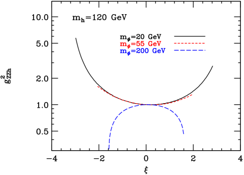
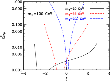
Figure 12: In the left figure, we plot $g_{ZZh}^{2}/g_{ZZh_{SM}}^{2}=g_{f\overline{f}h}^{2}/g_{f\overline{f}h_{SM}}^{2}$ as a function of $\xi$ for several $m_{\phi}$ values. The right figure shows $g_{ZZ\phi}^{2}/g_{ZZh_{SM}}^{2}=g_{f\overline{f}\phi}^{2}/g_{f\overline{f}h_{SM}}^{2}$.

The behavior of $g_{fVh}^{2}$ and $g_{fV\phi}^{2}$ is illustrated in Fig. 12. Some important general features of these couplings are the following. First, if $g_{fVh}^{2}<1$ ($g_{fVh}^{2}>1$) is observed then $m_{\phi}>m_{h}$ ($m_{\phi}<m_{h}$), respectively, except for a small region near $\xi=0$. For $m_{\phi}>m_{h}$, the suppression is most severe for large $|\xi|$ where $g_{fVh}^{2}\sim 0.1\div 0.2$ is possible. Second, for any given $m_{h}$, $g_{fV\phi}$ can be quite small and even has zeroes as one scans over the allowed $\xi$ range at a given $m_{\phi}$. However, at large $|\xi|$, if $m_{\phi}>m_{h}$ then $g_{fV\phi}$ can be a substantial fraction of the SM strength, $g_{fV\phi}=1$, implying SM type discovery modes could become relevant. The most important result of this is that $gg\to\phi\to ZZ\to 4\ell$ can be a viable discovery mode when $m_{\phi}\mathrel{\raise 1.29167pt\hbox{$>$\kern-7.5pt\lower 4.30554pt\hbox{$\sim$}}}2m_{Z}$ and $|\xi|$ is near the maximum allowed.

The universal scaling of the $f\overline{f}$ and $VV$ couplings of the $h$ and $\phi$ relative to the SM $h_{SM}$ implies that, unless these couplings are very suppressed, the $h$ and $\phi$ will have branching ratios that are quite SM-like. The only exceptions are the following. (1) Decays of the type $h\to\phi\phi$ can be significant at larger $\xi$ when $m_{\phi}$ is modestly below the $m_{h}/2$ threshold — $BR(h\to\phi\phi)_{\rm max}<0.2$ is typical for $\Lambda_{\phi}>5~{}{\rm TeV}$ and large $|\xi|$. (2) Where $g_{fV\phi}$ is near a zero, $\phi\to gg$ decays, induced by the anomalous coupling, will dominate. (3) For $m_{\phi}>2m_{h}$, $BR(\phi\to hh)\sim 0.3\div 0.5$ is typical. Of course, the total width of the $h$ or $\phi$ will be scaled down relative to an $h_{SM}$ of the same mass when $g_{fVh}^{2}<1$ or $g_{fV\phi}^{2}<1$ (respectively).

III.5.2 Numerical Results: LHC and $\gamma$C

In order to illustrate the complementarity of the LHC and $\gamma$C we will focus on the case $m_{h}=120~{}{\rm GeV}$, $\Lambda_{\phi}=5~{}{\rm TeV}$ and $m_{0}/M_{Pl}=0.1$. Once these parameters are fixed, the remaining free parameters are $m_{\phi}$ and $\xi$. of the results found there.

To illustrate the impact of the couplings on the standard LHC discovery modes, we give two plots. In Fig. 13 we see that the $h\to\gamma\gamma$ mode can be greatly suppressed if $m_{\phi}>m_{h}$, especially if $\xi<0$. Also, if $m_{\phi}<m_{h}$, $h\to\gamma\gamma$ will be strong if $\xi<0$, but can be considerably weakened if $\xi>0$. From Fig. 14, we observe that the discovery mode $gg\to\phi\to ZZ\to 4\ell$ can approach SM level viability at the largest allowed $|\xi|$ values, especially for $\xi<0$.

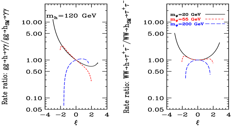
Figure 13: The ratios $gg\to h\to\gamma\gamma/gg\to h_{SM}\to\gamma\gamma$ and $WW\to h\to\tau^{+}\tau^{-}/WW\to h_{SM}\to\tau^{+}\tau^{-}$ (the latter being the same as for $gg\to t\overline{t}h\to t\overline{t}b\overline{b}$) for $m_{h_{SM}}=m_{h}=120~{}{\rm GeV}$ and $\Lambda_{\phi}=5~{}{\rm TeV}$.

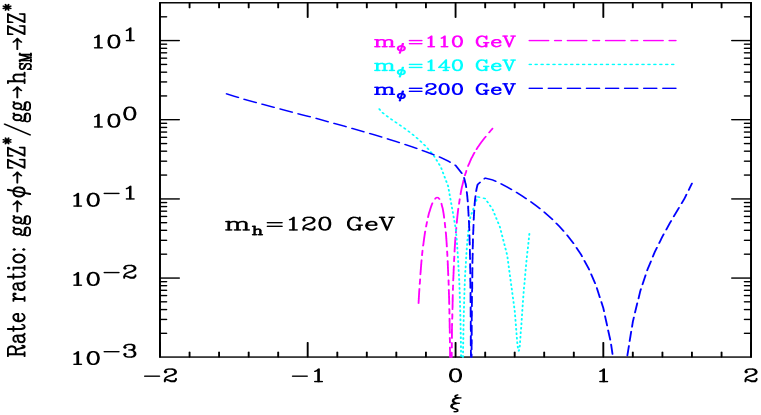
Figure 14: The ratio of the rate for $gg\to\phi\to ZZ$ to the corresponding rate for a SM Higgs boson with mass $m_{\phi}$ assuming $m_{h}=120~{}{\rm GeV}$ and $\Lambda_{\phi}=5~{}{\rm TeV}$ as a function of $\xi$ for $m_{\phi}=110$, $140$ and $200~{}{\rm GeV}$. Recall that the $\xi$ range is increasingly restricted as $m_{\phi}$ becomes more degenerate with $m_{h}$. Note: for $m_{\phi}>m_{h}$ the mode approaches SM strength if $\xi<0$ and is nearing SM strength if $\xi>0$ and near maximal.

A study of the resulting LHC prospects for $h$ and $\phi$ detection was performed in Battaglia:2003gb . Based on the preceding discussion, it should be possible to understand the features of Fig. 15 where we show the regions of $(m_{\phi},\xi)$ parameter space in which $h$ and/or $\phi$ discovery using LHC modes, designed for SM Higgs boson discovery, will be possible. The results are obtained by simply rescaling the signal rates for a SM Higgs boson of the same mass as the $h$ or $\phi$ using the type of rescaling factors plotted in Figs. 13 and 14.

Figure 15: Illustration of mode complementarity at the LHC for $m_{h}=120~{}{\rm GeV}$. The outer hourglass shape defines the theoretically allowed region in the $(m_{\phi},\xi)$ parameter space. The cyan regions show where neither the $gg\to h\to\gamma\gamma$ mode nor the (not very important at this $m_{h}$ value) $gg\to h\to 4\ell$ mode yields a $>5\sigma$ signal. LHC discovery of the $h$ with $>5\sigma$ is possible throughout the white region within the hourglass-shaped boundary. The graphs are for $\Lambda_{\phi}=5~{}{\rm TeV}$ and $L=30~{}{\rm fb}^{-1}$ (left) and $L=100~{}{\rm fb}^{-1}$ (right). In the left-hand, $L=30~{}{\rm fb}^{-1}$ plot, the regions between the dark blue curves are those where $gg\to\phi\to 4\ell$ is $>5\sigma$. These regions expand somewhat as $L$ increases. These figures are taken from Battaglia:2003gb .

Fig. 15 exhibits regions of $(m_{\phi},\xi)$ parameter space in which both the $h$ and $\phi$ mass eigenstates will be detectable. In these regions, the LHC will observe two scalar bosons somewhat separated in mass, with the lighter (heavier) having a non-SM-like rate for the $gg$-induced $\gamma\gamma$ ($Z^{0}Z^{0}$) final state. Additional information will be required to ascertain whether these two Higgs bosons derive from a multi-doublet or other type of extended Higgs sector or from the present type of model with Higgs-radion mixing.

If a linear collider is constructed, there is no region of $(m_{\phi},\xi)$ parameter space for which the $h$ (assuming modest $m_{h}$) will not be detected. This is because the $ZZh$ coupling strength is always such that $g_{fVh}^{2}>0.01$ (a value easily probed at the LC in the $e^{+}e^{-}\to ZX$ missing mass discovery mode). Depending on $m_{\phi}$, the $\phi$ will also be detectable in the $ZX$ final state if $g_{fV\phi}^{2}>0.01$. In particular, LC observation of the $\phi$ should be possible in the region of low $m_{\phi}$, large $\xi>0$ within which detection of either at the LHC might be difficult. This is because the $ZZ\phi$ coupling-squared is $\mathrel{\raise 1.29167pt\hbox{$>$\kern-7.5pt\lower 4.30554pt\hbox{$\sim$}}}0.01$ relative to the SM for most of this region.

However, let us imagine that the LC has not yet been built but that a photon-collider add-on to the CLIC test machine has been constructed. Let’s remind ourselves about the results for the SM Higgs boson obtained in the CLIC study of cliche . There, a SM Higgs boson with $m_{h_{SM}}=115~{}{\rm GeV}$ was examined. After the cuts, one obtains about $S=3280$ and $B=1660$ in the $\gamma\gamma\to h_{SM}\to b\overline{b}$ channel, corresponding to $S/\sqrt{B}\sim 80$!

We will assume that these numbers do not change significantly for a Higgs mass of $120~{}{\rm GeV}$. After mixing, the $S$ rate for the $h$ will be rescaled relative to that for the $h_{SM}$. Of course, $B$ will not change. The rescaling is shown in Fig. 16. The $S$ for the $\phi$ can also be obtained by rescaling if $m_{\phi}\sim 115~{}{\rm GeV}$. For $m_{\phi}<120~{}{\rm GeV}$, the $\phi\to b\overline{b}$ channel will continue to be the most relevant for $\phi$ discovery, but studies have not yet been performed to obtain the $S$ and $B$ rates for low masses.

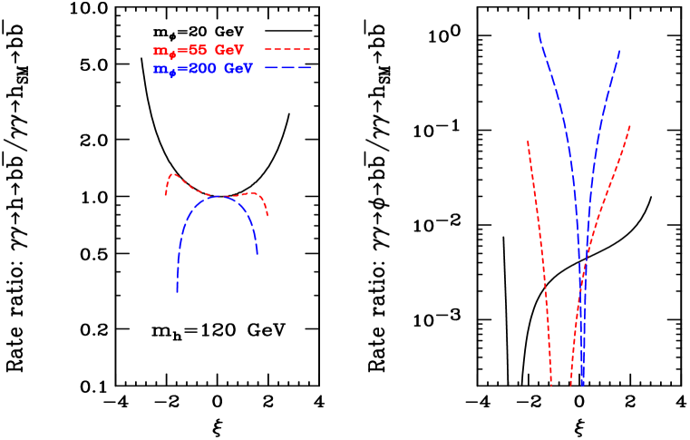
Figure 16: The rates for $\gamma\gamma\to h\to b\overline{b}$ and $\gamma\gamma\to\phi\to b\overline{b}$ relative to the corresponding rate for a SM Higgs boson of the same mass. Results are shown for $m_{h}=120~{}{\rm GeV}$ and $\Lambda_{\phi}=5~{}{\rm TeV}$ as functions of $\xi$ for $m_{\phi}=20$, $55$ and $200~{}{\rm GeV}$.

Observe that for $m_{\phi}<m_{h}$ we have either little change or enhancement, whereas significant suppression of the $gg\to h\to\gamma\gamma$ rate was possible in this case for positive $\xi$. Also note that for $m_{\phi}>m_{h}$ and large $\xi<0$ (where the LHC signal for the $h$ is marginal) there is much less suppression of $\gamma\gamma\to h\to b\overline{b}$ than for $gg\to h\to\gamma\gamma$ — at most a factor of 2 vs a factor of 8 (at $m_{\phi}=200~{}{\rm GeV}$). This is no problem for the $\gamma$C since $S/\sqrt{B}\sim{\textstyle{1\over 2}}80\sim 40$ is still a very strong signal. In fact, we can afford a reduction by a factor of $16$ before we hit the $5\sigma$ level! Thus, the $\gamma\gamma$ collider will allow $h$ discovery (for $m_{h}=120$) throughout the entire hourglass, which is something the LHC cannot absolutely do.

Using the factor of $16$ mentioned above and referring to the rescaling factors plotted in Fig. 14, it is apparent that the $\phi$ with $m_{\phi}<120~{}{\rm GeV}$ is very likely to elude discovery at the $\gamma\gamma$ collider. (Recall that it also eludes discovery at the LHC for this region.) The only exceptions to this statement occur at the very largest $|\xi|$ values for $m_{\phi}\geq 55~{}{\rm GeV}$ where $S_{\phi}>S_{h_{SM}}/16$.

Of course, we need to have signal and background results after cuts for these lower masses to know if the factor of 16 is actually the correct factor to use. To get the best signal to background ratio we would want to lower the machine energy (as would be relatively easy at a CLIC test facility) and readjust cuts and so forth. This study should be done. For the $m_{\phi}>m_{h}$ region, we will need results for the $WW$ and $ZZ$ modes that are being worked on.

III.5.3 Conclusions and discussion for Higgs-Radion Mixing

Overall, the $\gamma C$ is more than competitive with the LHC for $h$ discovery. In particular, the $\gamma C$ can see the $h$ where the LHC signal will be marginal (i.e. at the largest theoretically allowed $\xi$ values). Of course, the marginal LHC regions are not very big for full $L$. Perhaps even more interesting is the fact that there is a big part of the hourglass where the $h$ will be seen at both colliders. When the LHC achieves $L>100~{}{\rm fb}^{-1}$, this comprises most of the hourglass. Simultaneous observation of the $h$ at the two different colliders will greatly increase our knowledge about the $h$ since the two rates measure different things. The LHC rate in the $\gamma\gamma$ final state measures $\Gamma(h\to gg)\Gamma(h\to\gamma\gamma)/\Gamma_{\rm tot}^{h}$ while the $\gamma$C rate in the $b\overline{b}$ final state determines $\Gamma(h\to\gamma\gamma)\Gamma(h\to b\overline{b})/\Gamma_{\rm tot}^{h}$. Consequently, the ratio of the rates gives us ${\Gamma(h\to gg)\over\Gamma(h\to b\overline{b})}\,,$ in terms of which we may compute

$$R_{hgg}\equiv\left[{\Gamma(h\to gg)\over\Gamma(h\to b\overline{b})}\right]\left[{\Gamma(h\to gg)\over\Gamma(h\to b\overline{b})}\right]^{-1}_{SM}\,.$$ (19)

This is a very interesting number since it directly probes for the presence of the anomalous $ggh$ coupling. In particular, $R_{hgg}=1$ if the only contributions to $\Gamma(h\to gg)$ come from quark loops and all quark couplings scale in the same way. A plot of $R_{hgg}$ as a function of $\xi$ for $m_{h}=120~{}{\rm GeV}$, $\Lambda_{\phi}=5~{}{\rm TeV}$ and $m_{\phi}=20$, $55$ and $200~{}{\rm GeV}$ appears in Fig. 17.

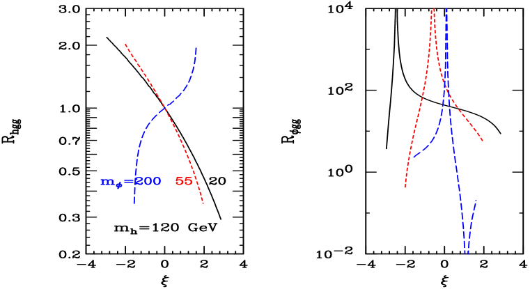
Figure 17: We plot the ratios $R_{hgg}$ and $R_{\phi gg}$ of the $hgg$ and $\phi gg$ couplings-squared including the anomalous contribution to the corresponding values expected in its absence. Results are shown for $m_{h}=120~{}{\rm GeV}$ and $\Lambda_{\phi}=5~{}{\rm TeV}$ as functions of $\xi$ for $m_{\phi}=20$, $55$ and $200~{}{\rm GeV}$. (The same type of line is used for a given $m_{\phi}$ in the right-hand figure as is used in the left-hand figure.)

We can estimate the accuracy with which $R_{hgg}$ can be measured as follows. Assuming the maximal reduction of 1/2 for the signal rate ($S$) rescaling at the $\gamma\gamma$ CLIC collider, we find that $\Gamma(h\to\gamma\gamma)\Gamma(h\to b\overline{b})/\Gamma_{tot}^{h}$ can be measured with an accuracy of about $\sqrt{S+B}/S\sim\sqrt{3200}/1600\sim 0.035$. The dominant error will then be from the LHC which will typically measure $\Gamma(h\to gg)\Gamma(h\to\gamma\gamma)/\Gamma_{tot}^{h}$ with an accuracy of between $0.1$ and $0.2$ (depending on parameter choices and available $L$). From Fig. 17, we see that $0.2$ fractional accuracy will reveal deviations of $R_{hgg}$ from $1$ for all but the smallest $\xi$ values. The ability to measure $R_{hgg}$ with good accuracy may be the strongest reason in the Higgs context for having the $\gamma C$ as well as the LHC. Almost all non-SM Higgs theories predict $R_{hgg}\neq 1$ for one reason another, unless one is in the decoupling limit.

Depending on $L$ at the LHC, there might be a small part of the hourglass (large $|\xi|$ with $m_{\phi}>m_{h}$) where only the $\phi$ will be seen at the LHC and the $h$ will only be seen at the $\gamma C$. This is a nice example of complementarity between the two machines. By having both machines we maximize the chance of seeing both the $h$ and $\phi$.

As regards the $\phi$, we have already noted from Fig. 16 that the $b\overline{b}$ final state rate (relevant for the $m_{\phi}=20$ and $55~{}{\rm GeV}$ cases) will only be detectable in the latter case (more generally for $55~{}{\rm GeV}<m_{\phi}<2m_{W}$), and then only if $|\xi|$ is as large as theoretically allowed. If $\gamma\gamma\to\phi\to b\overline{b}$ can be observed, Fig. 17 shows that a large deviation for $R_{\phi gg}$ relative to the value predicted for an $h_{SM}$ of the same mass is typical (but not guaranteed). For $m_{\phi}>2m_{W}$, $BR(\phi\to b\overline{b})$ will be very small and detection of $\gamma\gamma\to\phi\to b\overline{b}$ will not be possible. We are currently studying $\gamma\gamma\to\phi\to WW,ZZ$ final states in order to assess possibilities at larger $m_{\phi}$.

Overall, there is a strong case for the $\gamma C$ in the RS model context, especially if a Higgs boson is seen at the LHC that has non-SM-like rates and other properties.

IV Outlook

Important progress in establishing the TBA technique has been made over the last 7 years with the various CLIC Test facilities, and a Technical Design Report for a machine based on TBA technology could be available by 2008. The next technological step toward a multi-TeV collider could be the construction and operation of several full CLIC modules, each of them providing acceleration by about 70 GeV in 600 m, or even think of a staged program with different physics capablities that will eventually take us to a multi-TeV machine. Some of this could be running at the $Z$, $WW$ and/or $t\bar{t}$ threshold, etc.

By the time one would have to decide on the physics program of the initial stages of CLIC, it will be clear from the LHC if the Higgs exists, and if it is within the mass reach of CLICHE. Under this circumtances, CLICHE will have a strong motivation because it could provide complementary information on the Higgs boson from that obtained at the LHC, and help to distinguish among models.

In addition, the experience on a $\gamma$C that could be gained at a dedicated facility such as CLICHE will be very useful in order to learn how to operate what eventually will be a multi-TeV collider based on TBA technology just like CLIC MultiTeVGG .

It is true that CLICHE is only one of several options for doing physics with a limit number of CLIC modules. However, we consider CLICHE to be a very attractive option for an early stage of a TBA machine because it could simultaneously test all components for accelerating high-energy beams, and in addition it can give important scientific output. CLICHE could provide unique information on the properties of the Higgs boson, whose study will be central to physics at the high-energy physics frontier over the next decade or two.