Large Beyond–Leading–Order Effects in $b\rightarrow s\gamma$
in Supersymmetry with General Flavor Mixing

Abstract:

We examine squark–gluino loop effects on the process $b\rightarrow s\gamma$ in minimal supersymmetry with general flavor mixing in the squark sector. In the regime of heavy squarks and gluino, we derive analytic expressions for the beyond–LO corrections to the Wilson coefficients and find them to be often large, especially at large $\tan\beta$ and $\mu>0$. The ensuing ranges of values of the Wilson coefficients are typically smaller than in the LO approximation, and sometimes even change sign. This has the effect of often reducing, relative to the LO, the magnitude of supersymmetric contributions to $BR(B\rightarrow X_{s}\gamma)$. This “focusing effect” is caused by contributions from: (i) an RG evolution of the Wilson coefficients; (ii) a correction to the LO chargino contribution to the Wilson coefficients, which can considerably reduce the LO gluino contribution. This partial cancellation of the two contributions takes place only in the case of general flavor mixing. As a result, stringent lower bounds on the mass scale of superpartners, which apply in the case of minimal flavor violation, can be substantially reduced for even small departures from the scenario. The often disfavored case of $\mu<0$ can also become allowed for $M_{\rm SUSY}$ as small as $\sim 200\,\mbox{GeV}$, compared to $\mathrel{\hbox to0.0pt{\lower 4.0pt\hbox{\hskip 1.0pt$\sim$}\hss}\raise 1.0pt\hbox{$>$}}500\,\mbox{GeV}$ at LO and over $2\,\mbox{TeV}$ in the case of minimal flavor violation. Limits on the allowed amount of flavor mixing among the 2nd and 3rd generation down–type squarks are also typically considerably weakened. The input CKM matrix element $K^{(0)}_{cb}$ can be larger than the experimental value by a factor of ten, or can be as small as zero.

1 Introduction

It has long been recognized that the inclusive process $B\rightarrow X_{s}\gamma$ plays a prominent role in testing “new physics” beyond the Standard Model (SM) [1]. In the SM the leading contribution comes from a virtual $W$–top (charm, up) quark loop, which is accompanied by a real photon with GIM suppression. New physics effects, which are also loop induced, can be of the same order if a mass scale associated with the new physics is not much larger than $m_{\rm W}$. This in particular is the case with softly broken low–energy supersymmetry (SUSY) where the scale of SUSY breaking $M_{\rm SUSY}$ is expected to be $\mathrel{\hbox to0.0pt{\lower 4.0pt\hbox{\hskip 1.0pt$\sim$}\hss}\raise 1.0pt\hbox{$<$}}{\cal O}(1\,\mbox{TeV})$ on the grounds of naturalness.

Over the last decade, experimental precision has improved considerably, and the world average of the measured branching ratio has now been determined with an uncertainty of some $10\%$,

$${BR(B\rightarrow X_{s}\gamma)}_{expt}=(3.34\pm 0.38)\times 10^{-4},$$ (1)

where results from four experiments [2], including a recent one from BaBar, have been taken into account [3].

Theoretical calculations in the SM have been performed in several steps [4, 5], including the full next–to–leading order (NLO) QCD correction which has recently been completed in [6], and have reached as similar precision

$${BR(B\rightarrow X_{s}\gamma)}_{SM}=(3.70\pm 0.30)\times 10^{-4}.$$ (2)

Given the approximate agreement of the SM prediction (2) with experiment (1), any possible “new physics” effects must now be confined to the remaining, relatively narrow, window of uncertainty. This is normally expected to impose severe constraint on extensions of the SM. For example, in the two Higgs doublet model (2HDM) extension of the SM, where full NLO QCD corrections have also been completed [7, 8, 9], this allows one to derive rather stringent lower limit on the mass of the charged Higgs. It is worth noting, however, that the limit becomes sizeably weaker when NLO QCD corrections are included, as compared with the leading order (LO) approximation [8]. This demonstrates the importance of NLO QCD corrections [7, 8] and NLO mass renormalization effects [9].

Supersymmetric contributions to $BR(B\rightarrow X_{s}\gamma)$ have not yet been calculated with a similar level of accuracy, although, since the first detailed LO analysis [10], much important work has been done towards reaching this goal [1]. On the other hand, one might argue that, given little room left for “new physics” contributions, it may actually not be essential to include NLO QCD and SUSY QCD corrections since all the relevant superpartners may anyway have to be heavy enough in order for the SUSY contributions to be suppressed. However, in this regime, the magnitude of SUSY contributions is often comparable with LO and NLO QCD corrections. Furthermore, in some cases separate SUSY effects may actually be quite large, but may approximately cancel each other, thus allowing for lower $M_{\rm SUSY}$.

More importantly, new effects are known to exist beyond LO, and these may significantly modify SUSY contributions which in the LO approximation appear to be large. One such important new effect is induced by squark–gluino loop corrections to quark masses and couplings. For example, the mass correction to the bottom quark can be of order $\sim 40\%$ in the regime of large $\tan\beta$ [11]. The same mechanism has also a strong impact on effective quark couplings to gauge and Higgs bosons and to superpartners [12, 13, 14, 15]. Its effect on $b\rightarrow s\gamma$ has been explored [14, 15] in the framework of minimal flavor violation (MFV) [16] (where one assumes that the CKM matrix is a unique source of flavor mixing among both quarks and squarks), and shown to be sizeable at large $\tan\beta$ and for large ratio of $M_{\rm SUSY}/m_{\rm W}$.

The MFV scenario has some appealing theoretical features and is also partially motivated by stringent constraints from the $K^{0}-\bar{K}^{0}$ system [17, 20, 18] on the allowed mixings among the squarks of the first two generations. On the other hand, it is hard to believe that MFV is strictly obeyed at the electroweak scale. It is usually assumed to hold at some high scale $\Lambda$, like the grand unification scale, in an attempt to relate soft SUSY breaking terms to the structure of the Yukawa sector. However, the assumptions of MFV are not RG–invariant and sizeable flavor–violating terms of order $\ln\left(\Lambda^{2}/m_{\rm W}^{2}\right)/\left(4\pi\right)^{2}$ are generated by the running from the scale $\Lambda$ to the electroweak scale. Further violations are also induced by threshold effects at the SUSY breaking scale $M_{\rm SUSY}\sim 1\,\mbox{TeV}$. It is therefore sensible to assume that MFV can be regarded as, at best, only an approximate scenario at the electroweak scale.

A broader framework is that of general flavor mixing (GFM) among squarks and/or among sleptons. Flavor mixings of this type are not protected by any known symmetry, and can in principle be large. As a result, without any additional ansatz, otherwise allowed contributions to, e.g., the processes such as $\mu\to e\gamma$ or $K^{0}-\bar{K}^{0}$ mixing can exceed experimental bounds by as much as several orders of magnitude [21]. In this case, experimental limits become an efficient tool in severely restricting possible mixings among scalar superpartners, especially between the 1st and 2nd generation, while still leaving considerable room for departures from the MFV scheme.

In the case of $b\rightarrow s\gamma$, going beyond the MFV framework has particularly important implications. While in the MFV case only the chargino and up–squark loop exchange contributes to the process, in going beyond MFV flavor–violating gluino (and, to a lesser extent, neutralino) and down–squark loop exchange diagrams start playing a substantial role. The importance of these additional diagrams has long been recognized [22], in part because of the gluino exchange enhancement by the strong coupling constant. Following the earlier work of [23, 17], it has more recently been carefully studied in the LO approximation [24], and also in some special cases beyond LO, e.g. in [25]. (For a clear and systematic discussion of SUSY contributions in the case of GFM see ref. [24].)

Given the fact that beyond–LO effects in $b\rightarrow s\gamma$ have been shown to be sizeable in MFV and that by going beyond MFV new important loop contributions appear, it is worthwhile to consider the role of beyond–LO effects in the framework of GFM among squarks, and to examine their impact on bounds on supersymmetric masses and other parameters. In particular, one may ask whether small departures from MFV assumptions lead to only small perturbations on the various bounds on SUSY derived in the case of MFV. We will show that this is not the case.

In the previous paper [26] we have presented our first results showing a strong impact of the squark–gluino loop corrections on $b\rightarrow s\gamma$ in the framework of GFM. We have pointed out that such beyond–LO effects have an important effect of generally reducing the magnitude of SUSY contribution to $BR(B\rightarrow X_{s}\gamma)$, especially at large $\tan\beta$ and for $\mu>0$. This effect of “focusing” on the SM value is already present at some level in the case of MFV but becomes strongly enhanced when GFM is allowed. This is because in this case large beyond–LO contributions from the chargino and the gluino can partially cancel each other. Furthermore, gluino–squark corrections typically reduce SUSY contributions to Wilson coefficients $C_{7,8}$ relative to the LO approximation. This effect comes in addition to the known effect of reducing the magnitude of the Wilson coefficients due to a resummation of QCD logarithms in RG–running between $M_{\rm SUSY}$ and $m_{\rm W}$ [14]. In addition, in the framework of GFM, large contributions to the chirality–conjugate Wilson coefficients $C_{7,8}^{\prime}$ due to chargino exchange are induced which can partially cancel the contribution from gluino exchange.

In this study, we present analytic expressions for dominant beyond–LO corrections to the Wilson coefficients for the process $b\rightarrow s\gamma$ in the Minimal Supersymmetric Standard Model (MSSM) with GFM in the squark sector. In addition to including the NLO contributions from the SM and the 2HDM and the full NLO QCD corrections from gluon exchange, we compute dominant NLO–level SUSY QCD effects to relevant SUSY contributions, which are enhanced by large–$\tan\beta$ factors. While the full two–loop calculation still remains to be performed (with the first step already undertaken in [27]), our goal is to calculate the terms which are likely to be dominant beyond LO due to being enhanced at large $\tan\beta$ and at large $M_{\rm SUSY}/m_{\rm W}$. We will work in the regime where all the colored superpartners are heavier than all the other states. We generalize the analyses of [28, 14, 15] to the case of GFM. In addition, we include in our analysis an NLO anomalous dimension, an NLO QCD matching condition and a resummation of $\tan\beta$–enhanced radiative corrections [15, 14], which all further improve the accuracy of our analysis. We use the squark mass eigenstate formalism which is more appropriate when squark off–diagonal terms are not assumed to be small. We thus do not use the mass insertion approximation, similarly as in ref. [24].

Our main results can be summarized as follows. In the framework of GFM, dominant $\tan\beta$–enhanced beyond–LO effects due to squark–gluino loop corrections are quite large and have a strong impact on the Wilson coefficients. Their main effect is that of: (i) reducing, relative to LO, the size of the Wilson coefficients $C_{7,8}$, and (ii) of generating additional contributions to the Wilson coefficients $C_{7,8}^{\prime}$ which can be of similar size. As a result, the total values of $C_{7,8}^{(\prime)}$ can significantly change. For $\mu>0$ these are usually have a smaller value, but not necessarily magnitude, relative to the LO. In fact, they can even change sign. (For $\mu<0$ the pattern is less clear but the effect often remains sizeable.) As a result, the supersymmetric contribution to $BR(B\rightarrow X_{s}\gamma)$ can often change dramatically, even for small mixings among down–type squarks.

Our analysis demonstrates that various bounds on SUSY parameters obtained in the context of the MFV framework at the same level of accuracy can be highly unstable against even even small departures from it. An additional effect is that of strongly relaxing upper limits on the allowed amount of mixing in the 2nd–3rd generation squark sector relative to the LO case. Another important implication of our analysis is that the elements of the input CKM matrix can be larger than the experimentally measured values by a factor as large as ten (which is significantly more than some $\sim 40\%$ obtained in [35] with a specific boundary condition at the GUT scale), or can be even zero, in which case the measured values of the CKM matrix would have a purely radiative origin [29].

The impact of large gluino–squark loops on Wilson coefficients, considered here for the process of $b\rightarrow s\gamma$, appears to be quite generic and is likely to play an important role in other rare processes involving the bottom quark [30].

The paper is organized as follows. In sec. 2 and in appendices A–B we provide a detailed discussion of the effect of the squark–gluino loop corrections on quark masses and couplings and on the squark sector. In sec. 3 we outline our procedure of computing the Wilson coefficients, and in sec. 4 we present their analytic expressions. Numerical effects are then presented in sec. 5 and our conclusions are summarized in sec. 6. Several useful formulae are collected in appendices C–E for completeness.

2 Effective Quark Mass in SUSY with General Flavor Mixing

We will first define an effective, supersymmetric, softly–broken model with general flavor mixing in the squark sector as the framework for our analysis. In particular, we will concentrate on the effect of the squark–gluino loop corrections to down–type quark mass matrix on other properties of the model, in particular on the squark sector, effective couplings and the CKM matrix. Unless otherwise stated, we will work in the $\overline{MS}$–scheme.

The quark mass terms in an effective Lagrangian in the super–CKM basis read

$$-{\cal L}_{q}^{\rm mass}=\mbox{\boldmath${\bar{d}}_{R}^{{\dagger}}m^{(0)}_{d}d_{L}$}+\mbox{\boldmath${\bar{d}}_{R}^{{\dagger}}\delta m_{d}d_{L}$}+\mbox{\boldmath${\bar{u}}_{R}^{{\dagger}}m^{(0)}_{u}u_{L}$}+\mbox{\boldmath${\bar{u}}_{R}^{{\dagger}}\delta m_{u}u_{L}$}+h.c.,$$ (3)

where $\mbox{\boldmath$d_{L}$}=\left({d_{L}}_{i}\right)$, $\mbox{\boldmath$d_{R}$}=\left({d_{R}}_{i}\right)$, are the down–quark fields, and $\mbox{\boldmath$u_{L}$}=\left({u_{L}}_{i}\right)$ and $\mbox{\boldmath$u_{R}$}=\left({u_{R}}_{i}\right)$ are up–type quark fields, with $\mbox{\boldmath$m^{(0)}_{{d,u}}$}={\left(m^{(0)}_{d,u}\right)}_{ij}=\left({m^{(0)}_{d,u}}_{ij}\right)$ ($i,j=1,2,3$) denoting their respective uncorrected, or “bare”, $3\times 3$ mass matrices. These are related to the respective input, or “bare”, Yukawa coupling matrices $Y^{(0)}_{d,u}$ in the usual way $\mbox{\boldmath$m^{(0)}_{d,u}$}=v_{d,u}\mbox{\boldmath$Y^{(0)}_{d,u}$}$, where $v_{d,u}\equiv\langle H_{d,u}^{0}\rangle$.

The mass corrections $\delta m_{d,u}$ arise from squark–gluino one–loop contributions. Of particular interest is the mass correction $\delta m_{d}$ since it is enhanced at large $\tan\beta$ [11] and/or in the case when left–right soft terms are large,

$$\mbox{\boldmath$\delta m_{d}$}=v_{d}\tan\beta\,\mbox{\boldmath$\delta Y^{(0)}_{d}$}+\mbox{\boldmath$\delta m_{d}^{\rm soft}$}.$$ (4)

Note that the latter are in general independent of the Yukawa coupling and can also be sizeable. An explicit expression for $\delta m_{d}$ and a self–consistent procedure for computing it will be given below. Analogous corrections in the up–quark sector are not enhanced by large $\tan\beta$–factors, although in general there could be a substantial effect from left–right soft terms.

The effective (physical) quark mass matrices $m_{d,u}$ in the super–CKM basis are given by

$$m_{d} = \mbox{\boldmath$m^{(0)}_{d}$}+\left(\frac{\alpha_{s}}{4\pi}\right)\mbox{\boldmath$\delta m_{d}$},$$ (5)

$$m_{u} = \mbox{\boldmath$m^{(0)}_{u}$}+\left(\frac{\alpha_{s}}{4\pi}\right)\mbox{\boldmath$\delta m_{u}$}.$$ (6)

Note that we have explicitely extracted the factor $\alpha_{/}4\pi$ in the expressions above in order to stress the order of the leading SUSY QCD (SQCD) one–loop correction. Subdominant effects, e.g., due to chargino–stop loops considered in [14], can be added linearly.

The effective (physical) quark mass matrices $m_{d,u}$ in the super–CKM basis are (by definition) diagonal:

$$m_{d} = \mbox{\boldmath$diag$}\left(m_{d_{i}}\delta_{ij}\right)=\mbox{\boldmath$diag$}\left(m_{d},m_{s},m_{b}\right),$$ (7)

$$m_{u} = \mbox{\boldmath$diag$}\left(m_{u_{i}}\delta_{ij}\right)=\mbox{\boldmath$diag$}\left(m_{u},m_{c},m_{t}\right),$$ (8)

where $m_{d,s,b}$ and $m_{u,c,t}$ denote the physical masses of the quarks. In contrast, in this basis the matrices $m^{(0)}_{d,u}$ will in general be non–diagonal, and so will $\delta m_{d,u}$.

The CKM matrix is defined as usual

$$\mbox{\boldmath$K=V_{u_{L}}V_{d_{L}}^{{\dagger}}$}.$$ (9)

The elements of $K$ are determined from experiment, except for a small loop correction which can be found in appendix A. The unitary matrices $V_{{d,u}_{L,R}}$ rotate the interaction basis’ quark fields ${d^{o}_{L}}_{i}$, ${d^{o}_{R}}_{i}$, ${u^{o}_{L}}_{i}$, ${u^{o}_{R}}_{i}$ to the mass eigenstates ${d_{L}}_{i}$, ${d_{R}}_{i}$, ${u_{L}}_{i}$, ${u_{R}}_{i}$ ($i=1,2,3$) in the physical super–CKM basis. For example, ${d_{L}}_{i}={V_{d_{L}}}_{ij}{d^{o}_{L}}_{j}$, ${u_{R}}_{i}={V_{u_{R}}}_{ij}{u^{o}_{R}}_{j}$ ($i,j=1,2,3$). Also $\mbox{\boldmath$m^{(0)}_{d}$}=\mbox{\boldmath$V_{d_{R}}\,m^{(0)o}_{d}\,V_{d_{L}}^{{\dagger}}$}$, where $m^{(0)o}_{d}$ stands for the down–quark “bare” mass matrix in the interaction basis, and analogously for the up–quarks.

For our purpose, it will be convenient to further introduce a “bare” super–CKM basis. It is the basis in which the “bare” mass matrices $m^{(0)}_{d,u}$ are diagonal. In the absence of the mass corrections $\delta m^{(0)}_{d,u}$, the “bare” and the physical mass matrices would of course coincide and their eigenvalues would be equal to the physical quark masses which we will treat as input. In other words, there would be no need to distinguish between the “bare” and the physical super–CKM basis. (In fact, this level of accuracy is sufficient to compute supersymmetric contributions to rare decays in the LO approximation.) Note however, that once the mass corrections are switched on, it will be the “bare” Yukawa couplings, which initially appear as free parameters in the theory, that will have to be adjusted to compensate for the loop corrections.

The “bare” CKM matrix is defined as $K^{(0)}=V^{(0)}_{u_{L}}V^{(0)\,{\dagger}}_{d_{L}}$, where $V^{(0)}_{{d,u}_{L,R}}$ denote the unitary matrices that would transform the “bare” down– and up–quark mass matrices in the interaction basis into a diagonal form, in analogy with the case of the corrected super–CKM basis. As we will see later, in the presence of the one–loop mass corrections, the elements of $K^{(0)}_{cb}$ and $K_{cb}$ (the latter being determined by experiment) can show large discrepancies, which can reach a factor of ten, or can be reduced down to zero.

Turning next to the squark sector, in the super–CKM basis spanned by the fields $\mbox{\boldmath$\widetilde{d}_{L}$}=\left({\widetilde{d}_{L_{i}}}\right)$, $\mbox{\boldmath$\widetilde{d}_{R}$}=\left({\widetilde{d}_{R_{i}}}\right)$ ($i=1,2,3$), and $\mbox{\boldmath$\widetilde{u}_{L}$}=\left({\widetilde{u}_{L_{i}}}\right)$, $\mbox{\boldmath$\widetilde{u}_{R}$}=\left({\widetilde{u}_{R_{i}}}\right)$, the mass terms in the Lagrangian read

$$-{\cal L}_{\widetilde{q},\,{\rm soft}}^{\rm mass}=\left(\mbox{\boldmath$\widetilde{d}_{L}^{{\dagger}}$},\mbox{\boldmath$\widetilde{d}_{R}^{{\dagger}}$}\right)\left(\mbox{\boldmath${\cal M}_{\widetilde{d}}^{2}$}\right)\left(\begin{array}[]{ll}\mbox{\boldmath$\widetilde{d}_{L}$}\\ \mbox{\boldmath$\widetilde{d}_{R}$}\end{array}\right)+\left(\mbox{\boldmath$\widetilde{u}_{L}^{{\dagger}}$},\mbox{\boldmath$\widetilde{u}_{R}^{{\dagger}}$}\right)\left(\mbox{\boldmath${\cal M}_{\widetilde{u}}^{2}$}\right)\left(\begin{array}[]{ll}\mbox{\boldmath$\widetilde{u}_{L}$}\\ \mbox{\boldmath$\widetilde{u}_{R}$}\end{array}\right).$$ (10)

The $6\times 6$ down–squark mass matrix ${\cal M}_{\widetilde{d}}^{2}$ and the up–squark matrix ${\cal M}_{\widetilde{u}}^{2}$ are decomposed into $3\times 3$ block sub–matrices as follows

$$\mbox{\boldmath${\cal M}_{\widetilde{d}}^{2}$}=\left(\begin{array}[]{ll}\mbox{\boldmath$m^{2}_{d,LL}$}+\mbox{\boldmath$F_{d,LL}$}+\mbox{\boldmath$D_{d,LL}$}{}{}&\mbox{\boldmath$m^{2}_{d,LR}$}+\mbox{\boldmath$F_{d,LR}$}\\ \left(\mbox{\boldmath$m^{2}_{d,LR}$}+\mbox{\boldmath$F_{d,LR}$}\right)^{\dagger}&\mbox{\boldmath$m^{2}_{d,RR}$}+\mbox{\boldmath$F_{d,RR}$}+\mbox{\boldmath$D_{d,RR}$}\end{array}\right),$$ (13)

$$\mbox{\boldmath${\cal M}_{\widetilde{u}}^{2}$}=\left(\begin{array}[]{ll}\mbox{\boldmath$m^{2}_{u,LL}$}+\mbox{\boldmath$F_{u,LL}$}+\mbox{\boldmath$D_{u,LL}$}{}{}&\mbox{\boldmath$m^{2}_{u,LR}$}+\mbox{\boldmath$F_{u,LR}$}\\ \left(\mbox{\boldmath$m^{2}_{u,LR}$}+\mbox{\boldmath$F_{u,LR}$}\right)^{\dagger}&\mbox{\boldmath$m^{2}_{u,RR}$}+\mbox{\boldmath$F_{u,RR}$}+\mbox{\boldmath$D_{u,RR}$}\end{array}\right).$$ (16)

The terms appearing in (13)–(16) are related to their more familiar counterparts in the interaction basis by the same unitary transformations $V_{{d,u}_{L,R}}$ that appear in the quark sector: squark fields transform in the same way as the respective quark fields from the interaction basis $\mbox{\boldmath$\widetilde{d}_{L}^{o}$}=\left(\widetilde{d}_{L_{i}}^{o}\right)$, $\mbox{\boldmath$\widetilde{d}_{R}^{o}$}=\left(\widetilde{d}_{R_{i}}^{o}\right)$ ($i=1,2,3$), and $\mbox{\boldmath$\widetilde{u}_{L}^{o}$}=\left(\widetilde{u}_{L_{i}}^{o}\right)$, $\mbox{\boldmath$\widetilde{u}_{R}^{o}$}=\left(\widetilde{u}_{R_{i}}^{o}\right)$ to the super–CKM basis which is spanned by $\widetilde{d}_{L,R}$ and $\widetilde{u}_{L,R}$. For example, $\mbox{\boldmath$\widetilde{d}_{L}$}=\mbox{\boldmath$V_{d_{L}}\widetilde{d}_{L}^{o}$}$ and $\mbox{\boldmath$\widetilde{u}_{L}$}=\mbox{\boldmath$V_{u_{L}}\widetilde{u}_{L}^{o}$}$, etc. If one writes the Lagrangian for the soft SUSY breaking terms in the interaction basis as

$$-{\cal L}_{\widetilde{q},\,{\rm soft}}^{o,\,\rm mass}= \mbox{\boldmath$\widetilde{d}_{L}^{o\,{\dagger}}m^{2}_{Q}\widetilde{d}_{L}^{o}$}+\mbox{\boldmath$\widetilde{d}_{R}^{o\,{\dagger}}m^{2}_{D}\widetilde{d}_{R}^{o}$}+\left[\mbox{\boldmath$\widetilde{d}_{L}^{o\,{\dagger}}$}\left(v_{d}\mbox{\boldmath$A_{d}^{o\,\ast}$}\right)\mbox{\boldmath$\widetilde{d}_{R}^{o}$}+h.c.\right]+$$ (17)

$$\mbox{\boldmath$\widetilde{u}_{L}^{o\,{\dagger}}m^{2}_{Q}\widetilde{u}_{L}^{o}$}+\mbox{\boldmath$\widetilde{u}_{R}^{o\,{\dagger}}m^{2}_{U}\widetilde{u}_{R}^{o}$}+\left[\mbox{\boldmath$\widetilde{u}_{L}^{o\,{\dagger}}$}\left(v_{u}\mbox{\boldmath$A_{u}^{o\,\ast}$}\right)\mbox{\boldmath$\widetilde{u}_{R}^{o}$}+h.c.\right],$$

then the soft mass terms appearing in the mass matrix ${\cal M}_{\widetilde{d}}^{2}$ are given as follows

$$\mbox{\boldmath$m^{2}_{d,LL}$}=\mbox{\boldmath$V_{{d}_{L}}m^{2}_{Q}V_{{d}_{L}}^{{\dagger}}$},$$ (18)

$$\mbox{\boldmath$m^{2}_{d,RR}$}=\mbox{\boldmath$V_{{d}_{R}}m^{2}_{D}V_{{d}_{R}}^{{\dagger}}$},$$ (19)

$$\mbox{\boldmath$m^{2}_{d,LR}$}=\mbox{\boldmath$V_{{d}_{L}}$}\left(v_{d}\mbox{\boldmath$A_{d}^{\ast}$}\right)\mbox{\boldmath$V_{{d}_{R}}^{{\dagger}}$},$$ (20)

and similarly for the up sector. (In particular, $\mbox{\boldmath$m^{2}_{u,RR}$}=\mbox{\boldmath$V_{{u}_{R}}m^{2}_{U}V_{{u}_{R}}^{{\dagger}}$}$). The matrices $m^{2}_{d\,u,LL}$ and $m^{2}_{d\,u,RR}$ are all hermitian and are in general non–diagonal, as are their counterpart soft mass parameters $m^{2}_{Q}$, $m^{2}_{D}$ and $m^{2}_{U}$ in (17). Note that $m^{2}_{d,LL}$ and $m^{2}_{u,LL}$ are related by $SU(2)_{L}$ invariance. Since in the interaction basis they are both equal to $m^{2}_{Q}$, in the super–CKM basis one finds $\mbox{\boldmath$m^{2}_{d,LL}$}=\mbox{\boldmath$K^{{\dagger}}m^{2}_{u,LL}K$}$.

The trilinear $3\times 3$ matrices $A_{d,u}$ that appear in the $LR$ soft terms are in general non–hermitian. Note that we do not assume $A_{d,u}$ to be necessarily proportional to their respective Yukawa couplings.

The $F$–terms are given by

$$\mbox{\boldmath$F_{d,LL}$}=\mbox{\boldmath${m_{d}^{(0)}}^{{\dagger}}m_{d}^{(0)}$},$$ (21)

$$\mbox{\boldmath$F_{d,RR}$}=\mbox{\boldmath$m_{d}^{(0)}{m_{d}^{(0)}}^{{\dagger}}$},$$ (22)

$$\mbox{\boldmath$F_{d,LR}$}=-\mu\tan\beta\,\mbox{\boldmath${m_{d}^{(0)}}^{{\dagger}}$},$$ (23)

and similarly for the up squarks (except $\mbox{\boldmath$F_{u,LR}$}=-\mu\cot\beta\,\mbox{\boldmath${m_{u}^{(0)}}^{{\dagger}}$}$). Note it is the “bare” mass matrices $m^{(0)}_{d,u}$ that appear in the $F$–terms. This is because these are derived from the superpotential which contains “bare” Yukawa couplings and other “bare” parameters. For this reason, in the super–CKM basis the $F$–terms are not diagonal, which will lead to important effects. On the other hand, the $D$–terms remain diagonal in flavor space. They read

$$\mbox{\boldmath$D_{d,LL}$}=m_{Z}\cos 2\beta\left[T_{3d}-Q_{d}\sin^{2}\theta_{W}\right]\mbox{\boldmath${\mathchoice{\rm 1\mskip-4.0mul}{\rm 1\mskip-4.0mul}{\rm 1\mskip-4.5mul}{\rm 1\mskip-5.0mul}}$},$$ (24)

$$\mbox{\boldmath$D_{d,RR}$}=\left(m_{Z}\cos 2\beta\,Q_{d}\sin^{2}\theta_{W}\right)\mbox{\boldmath${\mathchoice{\rm 1\mskip-4.0mul}{\rm 1\mskip-4.0mul}{\rm 1\mskip-4.5mul}{\rm 1\mskip-5.0mul}}$},$$ (25)

where $T_{3d}=-1/2$ and $Q_{d}=-1/3$ (and analogously for the up–sector, with $T_{3u}=1/2$ and $Q_{d}=2/3$).

The mass matrices ${\cal M}^{2}_{{\widetilde{d}}}$ (${\cal M}^{2}_{{\widetilde{u}}}$) in the super–CKM basis can be diagonalized by unitary matrices which are represented by two $6\times 3$ sub–matrices $\Gamma_{d\,L}$ and $\Gamma_{d\,R}$ ($\Gamma_{u\,L}$ and $\Gamma_{u\,R}$),

$$\left(\mbox{\boldmath$\Gamma_{d\,L}$},\mbox{\boldmath$\Gamma_{d\,R}$}\right)\mbox{\boldmath${\cal M}_{\widetilde{d}}^{2}$}\left(\begin{array}[]{l}\mbox{\boldmath$\Gamma_{d\,L}^{{\dagger}}$}\\ \mbox{\boldmath$\Gamma_{d\,R}^{{\dagger}}$}\end{array}\right)=\mbox{\boldmath$diag$}\left(m_{\widetilde{d}_{1}}^{2},\ldots,m_{\widetilde{d}_{6}}^{2}\right)$$ (26)

and

$$\left(\mbox{\boldmath$\Gamma_{u\,L}$},\mbox{\boldmath$\Gamma_{u\,R}$}\right)\mbox{\boldmath${\cal M}_{\widetilde{u}}^{2}$}\left(\begin{array}[]{l}\mbox{\boldmath$\Gamma_{u\,L}^{{\dagger}}$}\\ \mbox{\boldmath$\Gamma_{u\,R}^{{\dagger}}$}\end{array}\right)=\mbox{\boldmath$diag$}\left(m_{\widetilde{u}_{1}}^{2},\ldots,m_{\widetilde{u}_{6}}^{2}\right),$$ (27)

where $m_{\widetilde{d}_{I}}$ and $m_{\widetilde{u}_{I}}$ ($I=1,\ldots,6$) are the physical masses of the down–, $\mbox{\boldmath$\widetilde{d}$}=\left(\widetilde{d}_{I}\right)$, and up–type, $\mbox{\boldmath$\widetilde{u}$}=\left(\widetilde{u}_{I}\right)$, squark mass eigenstates, respectively. These are related to the corresponding fields $\widetilde{d}_{L,R},\widetilde{u}_{L,R}$ in the super–CKM basis by

$$\mbox{\boldmath$\widetilde{d}$}=\mbox{\boldmath$\Gamma_{d\,L,R}$}\>\mbox{\boldmath$\widetilde{d}_{L,R}$},~{}~{}~{}~{}~{}~{}~{}~{}~{}~{}~{}~{}~{}~{}~{}~{}\mbox{\boldmath$\widetilde{u}$}=\mbox{\boldmath$\Gamma_{u\,L}$}\>\mbox{\boldmath$\widetilde{u}_{L,R}$}.$$ (28)

We will also need squark mass eigenvalues and diagonalizing matrices in the limit of vanishing mass corrections $\delta m_{d,u}$. Squark mass matrices in this limit will be denoted by

$$\mbox{\boldmath${\cal M}_{\widetilde{d}}^{(0)\,2}$}=\mbox{\boldmath${\cal M}_{\widetilde{d}}^{2}$}\left(\mbox{\boldmath$\delta m_{d}$}\rightarrow\mbox{\boldmath$0$}\right),$$ (29)

$$\mbox{\boldmath${\cal M}_{\widetilde{u}}^{(0)\,2}$}=\mbox{\boldmath${\cal M}_{\widetilde{u}}^{2}$}\left(\mbox{\boldmath$\delta m_{u}$}\rightarrow\mbox{\boldmath$0$}\right).$$ (30)

Since in this limit the “bare” and the physical super–CKM bases coincide, the $F$–terms are now diagonal and are given by $\mbox{\boldmath$F_{d,LL}^{(0)}$}=\mbox{\boldmath$F_{d,RR}^{(0)}$}=\mbox{\boldmath$diag$}\left(m_{d}^{2},m_{s}^{2},m_{b}^{2}\right)$ and $\mbox{\boldmath$F_{d,LR}^{(0)}$}=-\mu\tan\beta\,\mbox{\boldmath$diag$}\left(m_{d},m_{s},m_{b}\right)$ (and analogously for the up–squarks). This is because the “bare” mass matrices $m^{(0)}_{d,u}$, that appear in the $F$–terms, are in this limit diagonal, with the physical quark masses along the diagonal.

We will further introduce the masses of the down– and up–type squarks, respectively, in the limit of vanishing mass corrections $\delta m_{d,u}$

$$m^{(0)}_{\widetilde{d}_{I}}=m_{\widetilde{d}_{I}}\left(\mbox{\boldmath$\delta m_{d}$}\rightarrow\mbox{\boldmath$0$}\right),~{}~{}~{}~{}~{}~{}~{}m^{(0)}_{\widetilde{u}_{I}}=m_{\widetilde{u}_{I}}\left(\mbox{\boldmath$\delta m_{u}$}\rightarrow\mbox{\boldmath$0$}\right)~{}~{}~{}~{}~{}~{}~{}(I=1,\ldots,6),$$ (31)

as well as the diagonalizing matrices $\mbox{\boldmath$\Gamma_{d\,L}^{(0)}$}=\mbox{\boldmath$\Gamma_{d\,L}$}\left(\mbox{\boldmath$\delta m_{d}$}\rightarrow\mbox{\boldmath$0$}\right)$ and $\mbox{\boldmath$\Gamma_{d\,R}^{(0)}$}=\mbox{\boldmath$\Gamma_{d\,R}$}\left(\mbox{\boldmath$\delta m_{d}$}\rightarrow\mbox{\boldmath$0$}\right)$, and analogously for the up–squarks.

We will now apply the above formalism to describe our procedure of computing the one–loop mass correction $\delta m_{d}$ (4). The relevant diagram is given by fig. 1 for which one obtains [35]

$$\left(\delta m_{d}\right)_{ij}=2C_{2}(3)\sum_{I=1}^{6}\left(\Gamma_{d\,R}^{\ast}\right)_{Ii}\left(\Gamma_{d\,L}\right)_{Ij}m_{\widetilde{g}}B_{0}({m^{2}_{\widetilde{g}}},m_{\widetilde{d}_{I}}^{2}),$$ (32)

where the quartic Casimir operator for $SU(3)$ is $C_{2}(3)=\frac{4}{3}$, $m_{\widetilde{g}}$ denotes the mass of the gluino and $B_{0}$ is one of the Passarino–Veltman functions which are collected in appendix C. (An analogous expression for the mass correction $\left(\delta m_{u}\right)_{ij}$ can be obtained from (32) by simply replacing $d\rightarrow u$ and $\widetilde{d}\rightarrow\widetilde{u}$.)

Figure 1: Gluino–squark correction to the down–type quark mass matrix. Direction of the arrows indicates chirality of the quark field.

In our analysis we take the physical masses $m_{d_{1,2,3}}$ as input. On the other hand, in computing the diagram of fig. 1, one uses the elements of the “bare” mass matrix $m^{(0)}_{d}$ and of the squark mass matrix ${\cal M}_{\widetilde{d}}^{2}$, which in turn are functions of $m^{(0)}_{d}$ and other “bare” parameters. The final result must be equal to the physical quark masses. This means that we need to employ an iterative procedure to simultaneously determine $m^{(0)}_{d}$, $\mbox{\boldmath$\delta m^{(0)}_{d}$}(\mbox{\boldmath$m^{(0)}_{d}$})$ and $\mbox{\boldmath${\cal M}_{\widetilde{d}}^{2}$}(\mbox{\boldmath$m^{(0)}_{d}$})$ to a desired level of accuracy.

In the first iteration one neglects $\delta m_{d}$ and thus identifies $m^{(0)}_{d}$ with $m_{d}$. One then computes $\delta m_{d}$ by applying (32) where the elements of the squark sector are determined by ${\cal M}_{\widetilde{d}}^{(0)\,2}$, and not by ${\cal M}_{\widetilde{d}}^{2}$. In other words, in evaluating (32) one initially makes the substitutions $m_{\widetilde{d}_{I}}\rightarrow m^{(0)}_{\widetilde{d}_{I}}$ and $\Gamma_{d\,RL}$ $\rightarrow$ $\Gamma^{(0)}_{d\,RL}$.

In the second step one uses $\delta m_{d}$ from the first step to compute $\mbox{\boldmath$m^{(0)}_{d}$}=\mbox{\boldmath$m_{d}$}-\left(\alpha_{s}/4\pi\right)\,\mbox{\boldmath$\delta m_{d}$}$. The new values of the elements of $m^{(0)}_{d}$ are then used in (13) and (26) to determine the new eigenvalues $m_{\widetilde{d}_{I}}$ ($I=1,\ldots,6$) and the new elements of $\Gamma_{d\,L}$ and $\Gamma_{d\,R}$. These are then used to compute $\delta m_{d}$ via (32) and $m^{(0)}_{d}$ in the third step, and so on. The procedure converges quite rapidly, although not as well at very large $\tan\beta$.

The above iterative procedure amounts to resumming $\tan\beta$ terms to all orders in perturbation theory. The importance of resummation has been stressed in [15, 14] for extending the validity of perturbative calculation to the case of large $\tan\beta$. Below we will provide a simple formula for $\tan\beta$–resummation effect on the bottom mass in the limit of MFV.

Squark–gluino loop corrections also modify various couplings involving gauge and Higgs bosons, as well as those of the chargino, neutralino and gluino fields. The effective couplings are summarized in the appendices A and B. They are computed in the same self–consistent way as the quark and squark masses and mixings.

We will now illustrate the above procedure of computing quark mass corrections in the limit of vanishing inter–generational mixings among quarks. Concentrating on the correction to the mass of the b–quark one obtains

$$\delta m_{b}=\left(\delta m_{d}\right)_{33}=C_{2}(3)\sin 2\theta_{\widetilde{b}}m_{\widetilde{g}}\left[B_{0}\left(m_{\widetilde{g}}^{2},m^{2}_{{\widetilde{b}}_{1}}\right)-B_{0}\left(m_{\widetilde{g}}^{2},m^{2}_{{\widetilde{b}}_{2}}\right)\right],$$ (33)

where now the two sbottom mass states are ${\widetilde{b}}_{1}={\widetilde{d}}_{3}$ and ${\widetilde{b}}_{2}={\widetilde{d}}_{6}$, and they result from the mixing of only the interaction states ${\widetilde{b}}_{L}$ and ${\widetilde{b}}_{R}$, with $\theta_{\widetilde{b}}$ denoting the mixing angle,

$$\left(\begin{array}[]{cc}{\bf\Gamma_{d\,L}},{\bf\Gamma_{d\,R}}\end{array}\right)=\left(\begin{array}[]{cc}\cos\theta_{\widetilde{b}}&\sin\theta_{\widetilde{b}}\\ -\sin\theta_{\widetilde{b}}&\cos\theta_{\widetilde{b}}\end{array}\right),~{}~{}~{}\sin 2\theta_{\widetilde{b}}=\frac{2\left({\cal M}^{2}_{{\widetilde{d}}}\right)_{36}}{m^{2}_{{\widetilde{b}}_{1}}-m^{2}_{{\widetilde{b}}_{2}}},$$ (34)

where $\left({\cal M}^{2}_{{\widetilde{d}}}\right)_{36}=\left(m_{d,LR}^{2}\right)_{33}+\left(F_{d,LR}\right)_{33}$. After some simple steps one obtains

$$\delta m_{b}=2C_{2}(3)\frac{\left({\cal M}^{2}_{{\widetilde{d}}}\right)_{36}}{m_{\widetilde{g}}}H_{2}\left(\frac{m^{2}_{{\widetilde{b}}_{1}}}{m_{\widetilde{g}}^{2}},\frac{m^{2}_{{\widetilde{b}}_{2}}}{m_{\widetilde{g}}^{2}}\right),$$ (35)

where the function $H_{2}$ is given by

$$H_{2}(x,y)=\frac{x\ln x}{(1-x)(x-y)}+\frac{y\ln y}{(1-y)(y-x)}.$$ (36)

In the regime of moderate to large $\tan\beta$, and after neglecting $\left(m_{d,LR}^{2}\right)_{33}$, one recovers a familiar expression [14, 15]

$$m_{b}=\left(\sqrt{2}m_{W}\frac{Y_{b}^{(0)}}{g}\right)\cos\beta\,\left(1+\epsilon_{b}\tan\beta\right)=m_{b}^{(0)}\left(1+\epsilon_{b}\tan\beta\right),$$ (37)

where $m_{b}^{(0)}$ is the “bare” bottom quark mass and $\epsilon_{b}$ is given by

$$\epsilon_{b}=-\frac{2\alpha_{s}}{3\pi}\frac{\mu}{m_{\widetilde{g}}}H_{2}\left(\frac{m^{2}_{{\widetilde{b}}_{1}}}{m_{\widetilde{g}}^{2}},\frac{m^{2}_{{\widetilde{b}}_{2}}}{m_{\widetilde{g}}^{2}}\right).$$ (38)

The resummation of large radiative corrections at large $\tan\beta$ [15, 14] to all orders in perturbation theory is in our case achieved by employing the iterative procedure described above. In the case of the b–quark mass considered here, after the first iteration one obtains $m^{(0)}_{b}(1^{\rm st})=m_{b}\left(1-\epsilon_{b}^{(1)}\tan\beta\right)$, where $\epsilon_{b}^{(1)}$ denotes the correction (38) obtained in the first step of iteration, where one makes the replacement $m_{{\widetilde{b}}_{1,2}}\rightarrow m^{(0)}_{{\widetilde{b}}_{1,2}}$. If one denotes by $\epsilon_{b}^{(k)}$ the correction (38) obtained in the $k$–th step of iteration then, after n steps one obtains

$$m^{(0)}_{b}(n^{\rm th})=m_{b}\left[1-\epsilon_{b}^{(n)}\tan\beta+\epsilon_{b}^{(n)}\epsilon_{b}^{(n-1)}\tan^{2}\beta+\ldots+\left(-1\right)^{n}\epsilon_{b}^{(n)}\epsilon_{b}^{(n-1)}\ldots\epsilon_{b}^{(1)}\tan^{n}\beta\right].$$ (39)

We will now discuss the case of MFV as a limit of the GFM scenario. While in the literature the notion of MFV is not unique, and often depends on a model, the scenario is usually defined as the one where, at some scale, the $LL$ and $RR$ soft mass matrices are proportional to the unit matrix and the $LR$ ones are proportional to the respective Yukawa matrices. A convenient basis here is the super–CKM basis [36] where the Yukawa matrices are diagonal. In this case MFV corresponds to all off–diagonal entries in the soft mass matrices being zero. Thus it is the off–diagonal elements of $m^{2}_{d\,u,LL}$, $m^{2}_{d\,u,RR}$ and $m^{2}_{d\,u,LR}$ which in this basis are responsible for flavor change [37]. This is because, in the super–CKM basis, the couplings of the neutral gauginos are flavor–diagonal while the mixing in the charged gaugino–quark–squark couplings are all set by the SM CKM matrix $K$.

As mentioned above, in the absence of quark mass loop corrections, there is no need to distinguish between the “bare” and the physical super–CKM basis. However, once these are taken into account, an ambiguity arises. In one approach, one can insist that the $LR$ soft mass matrices remain proportional to the “bare” Yukawa couplings, which now become modified with respect to their tree–level values. This view can be motivated by an underlying assumption that, at some high scale, the two sets of quantities are ultimately related. Alternatively, in a more phenomenological approach like this one, one can assume that the $LR$ soft mass matrices do not change and thus remain proportional to the physical Yukawa couplings (which are the same as the “bare” tree–level Yukawa couplings) which in the super–CKM basis give the physical masses of the quarks. Here we choose the latter option. Fortunately, the difference between the two choices is numerically small.

We thus define the MFV scenario as the one in which, in the physical super–CKM basis, one has

$$\mbox{\boldmath$m^{2}_{d,LL}$}\propto\mbox{\boldmath${\mathchoice{\rm 1\mskip-4.0mul}{\rm 1\mskip-4.0mul}{\rm 1\mskip-4.5mul}{\rm 1\mskip-5.0mul}}$},\ \ \ \ \mbox{\boldmath$m^{2}_{d,RR}$}\propto\mbox{\boldmath${\mathchoice{\rm 1\mskip-4.0mul}{\rm 1\mskip-4.0mul}{\rm 1\mskip-4.5mul}{\rm 1\mskip-5.0mul}}$},\ \ \ \ \mbox{\boldmath$m^{2}_{d,LR}$}\propto\mbox{\boldmath$m_{d}$}/v_{d},$$ (40)

and analogously for the up–sector. Note that in the last relation of eq. (40) one also assumes that $\mbox{\boldmath$A_{d,u}^{T}$}\propto\mbox{\boldmath$Y_{d,u}$}$ which in the case of GFM does not have to be the case.

In order to parametrize departures from the MFV scenario, it is convenient to introduce the following dimensionless ($3\times 3$ matrix) parameters $\mbox{\boldmath$\delta^{d}_{LL}$}=\left(\delta^{d}_{LL}\right)_{ij}$, $\delta^{d}_{LR}$, etc., where $i,j=1,2,3$,

$${\left(\delta^{d}_{LL}\right)}_{ij}=~{}~{}~{}~{}~{}\frac{{\left(m^{2}_{d,LL}\right)}_{ij}}{\sqrt{{\left(m^{2}_{d,LL}\right)}_{ii}{\left(m^{2}_{d,LL}\right)}_{jj}}},~{}~{}~{}{\left(\delta^{d}_{LR}\right)}_{ij}=\frac{{\left(m^{2}_{d,LR}\right)}_{ij}}{\sqrt{{\left(m^{2}_{d,LL}\right)}_{ii}{\left(m^{2}_{d,RR}\right)}_{jj}}},$$ (41)

as well as

$${\left(\delta^{d}_{RR}\right)}_{ij}=~{}~{}~{}~{}~{}\frac{{\left(m^{2}_{d,RR}\right)}_{ij}}{\sqrt{{\left(m^{2}_{d,RR}\right)}_{ii}{\left(m^{2}_{d,RR}\right)}_{jj}}},~{}~{}~{}{\left(\delta^{d}_{RL}\right)}_{ij}=\frac{{\left(m^{2}_{d,RL}\right)}_{ij}}{\sqrt{{\left(m^{2}_{d,RR}\right)}_{ii}{\left(m^{2}_{d,LL}\right)}_{jj}}},$$ (42)

and analogously for the up–sector. The $\delta$’s can be evaluated at any scale equal to or above the typical scale of the soft terms. We will compute them at the scale $M_{\rm SUSY}$ which we will assume to be the characteristic mass scale for the soft mass terms. Note that the definitions (41)–(42) remain the same with and without loop quark mass corrections and are therefore particularly convenient for comparing the effects of LO and dominant beyond–LO corrections to $BR(B\rightarrow X_{s}\gamma)$ considered here.

3 Outline of the Procedure

Before plunging into technical details, we will first provide a general outline of our procedure for treating beyond–LO corrections to $BR(B\rightarrow X_{s}\gamma)$ in the framework of GFM. One starts with an effective Lagrangian [38] evaluated at some scale $\mu_{\rm 0}$,

$${\cal L}=\frac{4G_{F}}{\sqrt{2}}K_{ts}^{\ast}K_{tb}\sum\left[C_{i}({\mu_{\rm 0}}){\it P}_{i}+C_{i}^{\prime}({\mu_{\rm 0}}){\it P}_{i}^{\prime}\right].$$ (43)

The Wilson coefficients $C_{i}(\mu_{\rm 0})$ and $C_{i}^{\prime}(\mu_{\rm 0})$ associated with the operators ${\it P}_{i}$ and their chirality–conjugate partners ${\it P}_{i}^{\prime}$ play the role of effective coupling constants. The $C_{i}^{\prime}$’s are obtained from $C_{i}$’s by a chirality exchange $L\leftrightarrow R$.

At $\mu_{\rm 0}={\mu}_{\rm W}$, the Wilson coefficient of the four–fermion operator $C_{2}$ has a tree level contribution. Dominant loop contributions determine the coefficients $C_{7,8}$ of the magnetic and chromomagnetic operators, respectively, which are also most sensitive to “new physics”. These coefficients mix with each other when they are next evolved by renormalization group equations (RGEs) from ${\mu}_{\rm W}$ down to ${\mu}_{\rm b}$. Then $BR(B\rightarrow X_{s}\gamma)$ is evaluated at ${\mu}_{\rm b}$ as described in [9], with updated numerical values for the “magic numbers” taken from [6].

3.1 SM and 2HDM Contributions

In the SM+2HDM, in addition to the $W$–loop, there is a charged Higgs boson $H^{-}$ contribution to $C_{7,8}$ which always adds constructively to the one from the SM. Both contribute to ${\it C}_{i}^{\prime}$ as well, but this is suppressed by $m_{s}/m_{b}$ and can be ignored. In contrast, this is not necessarily the case in SUSY extensions of the SM.

In the SM+2HDM case the sum in eq. (43) extends to eight, while in SUSY in general several additional operators arise [24]. In our analysis we will henceforth restrict ourselves to the “SM basis” of operators but will consider below to what extent it is justified to neglect the additional operators.

Corrections from hard gluons to the vertices involving the $W$–boson, $H^{-}$ and $G^{-}$ (where $G^{-}$ represents the unphysical scalar appearing in $R_{\xi}$ gauge) are evaluated at the scale ${\mu}_{\rm W}=m_{\rm W}$. In computing them we follow the NLO QCD calculation of the matching condition at ${\mu}_{\rm W}$ [7, 8].

3.2 SUSY Contributions

In SUSY, additional loop contributions arise from diagrams involving the chargino, neutralino and gluino exchange, along with appropriate squarks. Furthermore, as has been shown in [12, 15, 14], NLO SUSY QCD corrections to one–loop diagrams involving the gluino field can be as important as those involving hard gluons.

The diagrams involving a loop exchange of the wino and higgsino components of the charginos (the superpartners of the $W^{-}$ and the $H^{-}$) with the up–type squarks add to the SM part constructively or destructively, depending on the sign of $\mu$. The chargino/up–type squark exchange is the only SUSY contribution if one imposes MFV assumptions. In the case of GFM, the diagrams involving the exchange of the gluino (and neutralino) and down–type squarks with flavor violating squark mass mixings are also allowed and, as discussed in sec. 2, in general play a substantial role.

In the softly–broken low energy SUSY model, with either MFV or GFM, an additional complication arises that is related to the fact that several new mass scales appear which are associated with the masses of the contributing SUSY partners. In this analysis we will assume that all color–carrying superpartners (gluinos and squarks) are considerably heavier (by at least a factor of a few) than other states

$${\mu}_{\rm SUSY}\sim{\cal O}(m_{\widetilde{g}},m_{\widetilde{q}},m_{\widetilde{t}_{1}},m_{\widetilde{t}_{2}})\gg{\mu}_{\rm W}\sim{\cal O}(m_{\rm W},m_{\rm t},m_{H^{\pm}})\gg{\mu}_{\rm b}\sim{\cal O}(m_{\rm b}).$$ (44)

Such a hierarchy is often realized in low–energy effective models with a gravity–mediated SUSY breaking mechanism because of different RG evolution of soft mass parameters from the unification scale down. It thus appears justified to associate the heaviest superpartners with the SUSY soft–breaking scale $M_{\rm SUSY}$. In particular, we assume both superpartners of the top quark to be heavy. Below the scale ${\mu}_{\rm SUSY}=M_{\rm SUSY}$ we will then deal with an effective model with the gluino and squark fields decoupled. Their effect will nevertheless be present in modifying the couplings of the states below ${\mu}_{\rm SUSY}$.

As stated above, for the states at ${\mu}_{\rm W}$ ($W$, $G^{-}$ and $H^{-}$), the contributions to the Wilson coefficients are evaluated at ${\mu}_{\rm W}$. The beyond–LO SUSY QCD corrections to these vertices, which are of order ${\cal O}(\alpha_{s})$, are absorbed into the effective vertices involving Yukawa couplings by integrating out the gluino field using the effective coupling method which has been introduced in [28]. In our case, the effective couplings are computed at ${\mu}_{\rm SUSY}$ and then evolved down to ${\mu}_{\rm W}$ using RGEs for the SM QCD $\beta$–functions with six quark flavors. For simplicity, in the effective couplings we neglect the running of the Yukawa and gauge couplings other than $\alpha_{s}$. We have extended to the case of GFM in the squark sector the calculation of the effective vertices and of the complete NLO matching condition at ${\mu}_{\rm W}$ which in [28] has been done in the framework of MFV.

The contributions to the Wilson coefficients from the chargino, gluino and neutralino vertices, including NLO QCD and SUSY QCD corrections, are first evaluated at ${\mu}_{\rm SUSY}$ and then evolved down to ${\mu}_{\rm W}$ with the NLO anomalous dimension corresponding to six quark flavors [39], and with NLO QCD matching condition [41] at ${\mu}_{\rm SUSY}$ within the SM operator basis. The leading SUSY QCD corrections beyond LO to the vertices of the above superpartner have been computed in refs. [28, 14, 15] in the case of MFV. Here we extend the calculation to the case of GFM among squarks.

In light of the assumed mass hierarchy (44), the chargino, gluino and neutralino vertices all involve some massive ($\sim M_{\rm SUSY}$) fields. In this case expansion by external momentum is not justified and the effective coupling method, which has been applied above to the states at ${\mu}_{\rm W}$, cannot be used anymore [28]. In order to treat them properly, one would have to calculate full 2–loop diagrams involving heavy fields, which is beyond the scope of this study. This has not yet even been done in the less complicated case of MFV. Instead, in [14, 15] finite threshold corrections to the bottom quark Yukawa coupling, which are enhanced at large $\tan\beta$, have been considered in the case of MFV. Here we extend this method to the GFM scenario and compute $\tan\beta$–enhanced (and also A–term enhanced) finite threshold corrections to the matrix of the Yukawa couplings of the down–type quarks. (Analogous corrections to the up–type quarks are not enhanced at large $\tan\beta$, although can possibly be by the soft terms.) These beyond–LO corrections are likely to be dominant due to being enhanced by $\tan\beta$ factors relative to other corrections. As mentioned above, we introduce NLO resummation of QCD logarithms to $C_{7,8}$ and $C_{7,8}^{\prime}$ assuming the hierarchy (44). In computing the chargino, gluino and neutralino loop contributions we follow [41] in implementing NLO QCD matching conditions.

The full set of operators in the sum in (43) that arises in SUSY has been systematically analyzed in ref. [24]. Box diagrams involving the gluino field generate scalar and tensor type four–quark operators, which are absent in the SM, at the matching scale ${\mu}_{\rm SUSY}$. As a result of RG evolution from ${\mu}_{\rm SUSY}$ to ${\mu}_{\rm b}$, in contrast to the vector type operators in the SM, at 1–loop level these new operators mix with the magnetic and chromo–magnetic operators and the contribution due to the mixing from these new operators could be comparable to the initial loop contribution to the (chromo–) magnetic operators.

This mixing effect appears, however, to be subdominant at least at LO. In the presence of the new operators, the (chromo–)magnetic operators are classified as dimension 5 or 6 depending on whether the chirality flip of the operator originates from the mass of the gluino in the loop or from that of the external quark [24]. The new operators mix only with the dimension 6 operators and their contribution to the $b\rightarrow s\gamma$ amplitude is suppressed by $m_{b}/m_{\widetilde{g}}$ relative to that of the dimension 5 ones. Because the new operators always appear with the dimension 5 operators, which are generated by the same set of flavor mixing among squarks, their effect is subdominant. This suppression has been numerically confirmed in [24].

In the absence of the NLO anomalous dimensions, matrix elements, bremsstrahlung corrections and matching conditions for the complete set of operators, we are unable to evaluate their contribution at NLO at the same level of accuracy as for the SM set. However, the above suppression mechanism is based on the chirality structure and we can see no obvious reason for any sizeable enhancement from the new operators at NLO which would overcome an additional $\alpha_{s}$ suppression with respect to the already subdominant LO contribution. Based on the above argument, in this work we restrict ourselves to the SM set of operators.

4 Wilson coefficients

In this section, we present expressions for the supersymmetric contributions to $C_{7,}^{(\prime)}(\mu_{W})$ and $C_{8}(\mu_{W})$ obtained using the procedure outlined above.

In the MSSM, the Wilson coefficients for magnetic and chromo–magnetic operators $C_{7}$ and $C_{8}$, in addition to the $W^{-}$–$t$ and $H^{-}$–$t$ loops, receive contributions from the $\chi^{-}_{1,2}$–$\widetilde{u}_{1,\ldots,6}$, $\chi^{0}_{1,\ldots,4}$–$\widetilde{d}_{1,\ldots,6}$ and $\widetilde{g}$–$\widetilde{d}_{1,\ldots,6}$ loops,

$$C_{7,8}({\mu}_{\rm W})=\delta^{W}C_{7,8}({\mu}_{\rm W})+\delta^{H}C_{7,8}({\mu}_{\rm W})+\delta^{S}C_{7,8}({\mu}_{\rm W}),$$ (45)

where $S=\chi^{-},\chi^{0},\widetilde{g}$,

$$\delta^{S}C_{7,8}({\mu}_{\rm W})=\delta^{\chi^{-}}C_{7,8}({\mu}_{\rm W})+\delta^{\chi^{0}}C_{7,8}({\mu}_{\rm W})+\delta^{\widetilde{g}}C_{7,8}({\mu}_{\rm W}).$$ (46)

Analogous expressions apply to $C^{\prime}_{7,8}$ except for the cases explicitly mentioned below.

The coefficients $\delta^{X}C_{7,8}$, where $X=W,H$, including order $\alpha_{s}$ NLO QCD and SUSY QCD corrections are evaluated at ${\mu}_{\rm W}$

$$\delta^{X}C_{7,8}({\mu}_{\rm W})=\delta^{X}C^{(0)}_{7,8}({\mu}_{\rm W})+\frac{\alpha_{s}({\mu}_{\rm W})}{4\pi}\delta^{X}C^{(1)}_{7,8}({\mu}_{\rm W}),$$ (47)

where $\delta^{X}C^{(0)}_{7,8}$ and $\delta^{X}C^{(1)}_{7,8}$ denote the LO and NLO contributions, respectively.

The $H^{-}$ and $W^{-}$ contributions to the Wilson coefficients at ${\mu}_{\rm W}$ are matched with an effective theory with five quark flavors. Their LO contributions are given by [42, 28],

$$\delta^{W}C^{(0)}_{7,8}({\mu}_{\rm W}) = F^{(1)}_{7,8}\left(\frac{\overline{m}_{t}^{2}({\mu}_{\rm W})}{m_{W}^{2}}\right),$$ (48)

$$\delta^{H}C^{(0)}_{7,8}({\mu}_{\rm W}) = \frac{1}{3\tan^{2}\beta}F^{(1)}_{7,8}\left(\frac{\overline{m}_{t}^{2}({\mu}_{\rm W})}{m_{H}^{2}}\right)+F^{(2)}_{7,8}\left(\frac{\overline{m}_{t}^{2}({\mu}_{\rm W})}{m_{H}^{2}}\right),$$ (49)

where $\overline{m}_{t}({\mu}_{\rm W})$ is the $\overline{MS}$ running mass of top quark at ${\mu}_{\rm W}$ and $m_{H}$ denotes the mass of the charged Higgs. The mass functions $F^{(1,2)}_{7,8}$ are given in appendix D.

The NLO matching condition of the Wilson coefficients $\delta^{W,H}C^{(1)}_{7,8}$ at ${\mu}_{\rm W}$ reads

$$\delta^{W,H}C^{(1)}_{7,8}({\mu}_{\rm W})=\delta^{W,H}_{g}C_{7,8}^{(1)}({\mu}_{\rm W})+\delta^{W,H}_{\widetilde{g}}C_{7,8}^{(1)}({\mu}_{\rm W}),$$ (50)

where $\delta^{W,H}_{g}C_{7,8}^{(1)}$ represents an NLO QCD correction from two–loop diagrams involving one gluon line and analogously $\delta^{W,H}_{\widetilde{g}}C_{7,8}^{(1)}$ stand for corrections from two–loop diagrams with a gluino line, which are integrated out at ${\mu}_{\rm SUSY}$. Explicit expressions for $\delta^{W,H}_{g}C^{(1)}_{7,8}$ are given in refs. [28, 41] and collected in appendix E.

As outlined in sec. 3, in computing $\delta^{W,H}_{\widetilde{g}}C_{7,8}^{(1)}$ we use the effective coupling method [28] and replace in the relevant LO diagrams the tree–level couplings for the $W^{-}$ ($G^{-}$) and $H^{-}$ vertices by corresponding effective couplings. These are given in appendix A and are first computed in the regime of eq. (44) at ${\mu}_{\rm SUSY}$ and next evolved down to ${\mu}_{\rm W}$ using RGEs with SM QCD $\beta$–functions. The effect of the running of the Yukawa and gauge couplings other than $\alpha_{s}$ is neglected as subdominant. One finally obtains

$$\delta^{W}_{\widetilde{g}}C_{7,8}^{(1)}({\mu}_{\rm W}) = \frac{2}{3g_{2}^{2}K^{\ast}_{ts}K_{tb}}\frac{{m_{\rm W}}^{2}}{\overline{m}_{t}^{2}({\mu}_{\rm W})}\times$$

$$\left[\left(C^{Gu_{3}d_{2}(0)\ast}_{L}C^{Gu_{3}d_{3}(1)}_{L}+C^{Gu_{3}d_{2}(1)\ast}_{L}C^{Gu_{3}d_{3}(0)}_{L}\right)F_{7,8}^{(1)}\left(\frac{\overline{m}_{t}^{2}({\mu}_{\rm W})}{{m_{\rm W}}^{2}}\right)\right.$$

$$\left.+\frac{\overline{m}_{t}}{\overline{m}_{b}({\mu}_{\rm W})}\left(C^{Gu_{3}d_{2}(0)\ast}_{L}C^{Gu_{3}d_{3}(1)}_{R}+C^{Gu_{3}d_{2}(1)\ast}_{L}C^{Gu_{3}d_{3}(0)}_{R}\right)F_{7,8}^{(2)}\left(\frac{\overline{m}_{t}^{2}({\mu}_{\rm W})}{{m_{\rm W}}^{2}}\right)\right],$$

$$\delta^{H}_{\widetilde{g}}C_{7,8}^{(1)}({\mu}_{\rm W}) = \frac{2}{3g_{2}^{2}K^{\ast}_{ts}K_{tb}}\frac{{m_{\rm W}}^{2}}{\overline{m}_{t}^{2}({\mu}_{\rm W})}\times$$

$$\left[(C^{Hu_{3}d_{2}(0)\ast}_{L}C^{Hu_{3}d_{3}(1)}_{L}+C^{Hu_{3}d_{2}(1)\ast}_{L}C^{Hu_{3}d_{3}(0)}_{L})F_{7,8}^{(1)}\left(\frac{\overline{m}_{t}^{2}({\mu}_{\rm W})}{m_{H}^{2}}\right)\right.$$

$$\left.+\frac{\overline{m}_{t}({\mu}_{\rm W})}{\overline{m}_{b}({\mu}_{\rm W})}(C^{Hu_{3}d_{2}(0)\ast}_{L}C^{Hu_{3}d_{3}(1)}_{R}+C^{Hu_{3}d_{2}(1)\ast}_{L}C^{Hu_{3}d_{3}(0)}_{R})F_{7,8}^{(2)}\left(\frac{\overline{m}_{t}^{2}({\mu}_{\rm W})}{m_{H}^{2}}\right)\right],$$

where $\overline{m}_{t}({\mu}_{\rm W})$ and $\overline{m}_{b}({\mu}_{\rm W})$ are $\overline{MS}$ running top and bottom masses at ${\mu}_{\rm W}$. Explicit expressions for the effective couplings $C^{Gu_{i}d_{j}(0,1)}_{L,R}$ and $C^{Gu_{i}d_{j}(0,1)}_{L,R}$ at ${\mu}_{\rm W}$ and other effective couplings are given in appendix A. Analogous expressions for $\delta^{W,H}C^{\prime}_{7,8}$ can be obtained by simply interchanging L and R in the formulae above.

In light of eq. (44), the LO and NLO supersymmetric contributions to the Wilson coefficients $\delta^{S}C_{7,8}$ are first computed at $\mu_{SUSY}$,

$$\delta^{S}C_{7,8}({\mu}_{\rm SUSY}) = \delta^{S}C^{(0)}_{7,8}({\mu}_{\rm SUSY})+\frac{\alpha_{s}({\mu}_{\rm SUSY})}{4\pi}\delta^{S}C^{(1)}_{7,8}({\mu}_{\rm SUSY}).$$ (53)

Next, they are evolved down to ${\mu}_{\rm W}$ with the QCD renormalization group equation. For this purpose we use the NLO anomalous dimension obtained in [39], assuming six quark flavors, and employ the NLO expression given in [40] for matrix evolution

$$\left(\begin{array}[]{c}\delta^{S}C_{7}({\mu}_{\rm W})\\ \delta^{S}C_{8}({\mu}_{\rm W})\end{array}\right)=\left(\mbox{\boldmath${\mathchoice{\rm 1\mskip-4.0mul}{\rm 1\mskip-4.0mul}{\rm 1\mskip-4.5mul}{\rm 1\mskip-5.0mul}}$}+\frac{\alpha_{s}({\mu}_{\rm W})}{4\pi}\mbox{\boldmath$J$}\right)\mbox{\boldmath$U^{(0)}$}\left(\mbox{\boldmath${\mathchoice{\rm 1\mskip-4.0mul}{\rm 1\mskip-4.0mul}{\rm 1\mskip-4.5mul}{\rm 1\mskip-5.0mul}}$}-\frac{\alpha_{s}({\mu}_{\rm SUSY})}{4\pi}\mbox{\boldmath$J$}\right)\left(\begin{array}[]{c}\delta^{S}C_{7}({\mu}_{\rm SUSY})\\ \delta^{S}C_{8}({\mu}_{\rm SUSY})\end{array}\right),$$ (54)

$$\mbox{\boldmath$U^{(0)}$}=\left(\begin{array}[]{rr}\eta^{\frac{16}{21}}&-\frac{8}{3}\left(\eta^{\frac{16}{21}}-\eta^{\frac{2}{3}}\right)\\ 0&\eta^{\frac{2}{3}}\end{array}\right),~{}~{}~{}~{}~{}\mbox{\boldmath$J$}=\left(\begin{array}[]{rr}-\frac{440}{49}&\frac{28136}{30429}\\ 0&-\frac{73}{9}\end{array}\right),$$ (55)

where $\eta=\alpha_{s}({\mu}_{\rm SUSY})/\alpha_{s}({\mu}_{\rm W})$. After extracting the LO and NLO parts of Wilson coefficients at both scales, eq. (54) reduces to a more familiar form in the case of six quark flavors,

$$\delta^{S}C^{(0)}_{7}({\mu}_{\rm W}) = \eta^{\frac{16}{21}}\delta^{S}C^{(0)}_{7}(\mu_{SUSY})+\frac{8}{3}\left(\eta^{\frac{2}{3}}-\eta^{\frac{16}{21}}\right)\delta^{S}C^{(0)}_{8}(\mu_{SUSY}),$$ (56)

$$\delta^{S}C^{(0)}_{8}({\mu}_{\rm W}) = \eta^{\frac{2}{3}}\delta^{S}C^{(0)}_{8}(\mu_{SUSY}),$$ (57)

$$\delta^{S}C^{(1)}_{7}({\mu}_{\rm W}) = +\frac{440}{49}\left(\eta^{\frac{37}{21}}-\eta^{\frac{16}{21}}\right)\delta^{S}C^{(0)}_{7}(\mu_{SUSY})$$ (58)

$$+\left(\frac{584}{27}\eta^{\frac{5}{3}}-\frac{76256}{3381}\eta^{\frac{37}{21}}-\frac{14296}{621}\eta^{\frac{2}{3}}+\frac{3520}{147}\eta^{\frac{16}{21}}\right)\delta^{S}C^{(0)}_{8}(\mu_{SUSY})$$

$$+\eta^{\frac{37}{21}}\delta^{S}C^{(1)}_{7}(\mu_{SUSY})+\frac{8}{3}\left(\eta^{\frac{5}{3}}-\eta^{\frac{37}{21}}\right)\delta^{S}C^{(1)}_{8}(\mu_{SUSY}),$$

$$\delta^{S}C^{(1)}_{8}({\mu}_{\rm W}) = \eta^{\frac{5}{3}}\delta^{S}C^{(1)}_{8}(\mu_{SUSY})+\frac{73}{9}\left(\eta^{\frac{5}{3}}-\eta^{\frac{2}{3}}\right)\delta^{S}C^{(0)}_{8}(\mu_{SUSY}).$$ (59)

While we work within the SM basis of operators, SUSY loop induced ${\it O}(\alpha_{s})$ contributions to $C_{i}$ ($i=1,\ldots,6$) at ${\mu}_{\rm SUSY}$ also in principle mix with $C_{7,8}$ during the course of evolution. However, the corresponding $P_{i}$ ($i=1,\ldots,6$) conserve chirality and are not enhanced by $\tan\beta$. We have numerically verified that their typical values are ${\cal O}(10^{-3})$–${\cal O}(10^{-4})$ if squarks/gluino masses are not very close to ${\mu}_{\rm W}$. Their contributions to $C_{7,8}$ are further suppressed by mixing factors. Because the purpose of this paper is to present large $\tan\beta$–enhanced beyond–leading–order effects in $BR(B\rightarrow X_{s}\gamma)$, for simplicity we neglect these small contributions compared to the ${\cal O}(10^{-1})$ SM ones.

The NLO supersymmetric contributions to the Wilson coefficients at ${\mu}_{\rm SUSY}$ reads

$$\delta^{S}C^{(1)}_{7,8}({\mu}_{\rm SUSY}) = \delta^{S}_{g}C_{7,8}^{(1)}({\mu}_{\rm SUSY})+\delta^{S}_{\widetilde{g}}C_{7,8}^{(1)}({\mu}_{\rm SUSY})~{}~{}~{}~{}~{}(S=\chi^{-},\chi^{0},\widetilde{g}),$$ (60)

where $\delta^{S}_{g}C_{7,8}^{(1)}$ and $\delta^{S}_{\widetilde{g}}C_{i}^{(1)}$ denote respective gluon and gluino NLO corrections, analogously to the $W$ and $H$ contributions at ${\mu}_{\rm W}$. Explicit expressions for $\delta^{S}_{g}C^{(1)}_{7,8}$ can be found in ref. [41] and appendix E.

Figure 2: Leading diagrams that contribute to $\delta^{\chi^{-}}_{\widetilde{g}}C_{7,8}^{(1)}$ (left) and $\delta^{\widetilde{g}}_{\widetilde{g}}C_{7,8}^{(1)}$ (right). The photon (or gluon) line is attached in every possible manner.

In computing gluino corrections to supersymmetric contributions $\delta^{S}_{\widetilde{g}}C_{7,8}^{(1)}$, the effective vertex method does not work, as explained in sec. 3. Instead of calculating the full two–loop diagrams, we take into account $\tan\beta$–enhanced corrections to the Yukawa couplings, as well as $LR$ mixings due to terms involving the trilinear soft terms $A_{d,u}$ which in principle can also be sizeable. In the absence of full 2–loop calculation of $C_{7,8}$, such effective Yukawa vertices contain only the dominant corrections. (In fig. 2 and 3, we show the Feynman diagrams that contribute the leading corrections to $C_{7,8}$.) We indicate the approximation by replacing $\delta^{S}_{\widetilde{g}}C_{7,8}^{(1)}\rightarrow\delta^{S}_{\widetilde{g}}C_{7,8}^{(Y)}$. We obtain

$$\left({\delta^{\chi^{-}}}C_{7,8}^{(0)}+\frac{\alpha_{s}}{4\pi}{\delta^{\chi^{-}}_{\widetilde{g}}}C_{7,8}^{(Y)}\right)({\mu}_{\rm SUSY}) = \frac{1}{g_{2}^{2}K^{\ast}_{ts}K_{tb}}\sum^{2}_{a=1}\sum^{6}_{I=1}\frac{m_{W}^{2}}{m_{\chi^{-}_{a}}^{2}}\times$$

$$\left[\left(C_{d\,R}\right)_{2aI}\left(C_{d\,R}\right)^{\ast}_{3aI}H_{1}^{[7,8]}\left(x^{{\widetilde{u}}_{I}}_{\chi^{-}_{a}}\right)\right.$$

$$\left.+\frac{m_{\chi^{-}_{a}}}{\overline{m}_{b}({\mu}_{\rm SUSY})}\left(C_{d\,R}\right)_{2aI}\left(C_{d\,L}\right)^{\ast}_{3aI}\left(H_{2}^{[7,8]}\left(x^{{\widetilde{u}}_{I}}_{\chi^{-}_{a}}\right)+\lambda^{[7,8]}\right)\right],$$

$$\left(\delta^{\chi^{0}}C_{7,8}^{(0)}+\frac{\alpha_{s}}{4\pi}\delta^{\chi^{0}}_{\widetilde{g}}C_{7,8}^{(Y)}\right)(\mu_{SUSY}) = \frac{1}{g_{2}^{2}K^{\ast}_{ts}K_{tb}}\sum^{4}_{r=1}\sum^{6}_{I=1}\frac{m_{W}^{2}}{m_{\chi^{0}_{r}}^{2}}\times$$

$$\left[\left(N_{d\,R}\right)_{2rI}\left(N_{d\,R}\right)^{\ast}_{3rI}H_{3}^{[7,8]}\left(x^{{\widetilde{d}}_{I}}_{\chi^{0}_{r}}\right)\right.$$

$$\left.+\frac{m_{\chi^{0}_{r}}}{\overline{m}_{b}({\mu}_{\rm SUSY})}\left(N_{d\,R}\right)_{2rI}\left(N_{d\,L}\right)^{\ast}_{3rI}H_{4}^{[7,8]}\left(x^{{\widetilde{d}}_{I}}_{\chi^{0}_{r}}\right)\right],$$

$$\left(\delta^{\widetilde{g}}C_{7,8}^{(0)}+\frac{\alpha_{s}}{4\pi}\delta^{\widetilde{g}}_{\widetilde{g}}C_{7,8}^{(Y)}\right)(\mu_{SUSY}) = \frac{4}{3g_{2}^{2}K^{\ast}_{ts}K_{tb}}\sum^{6}_{I=1}\frac{m_{W}^{2}}{m_{\widetilde{g}}^{2}}\times$$

$$\left[\left(G_{d\,R}\right)_{2I}\left(G_{d\,R}\right)^{\ast}_{3I}H_{5}^{[7,8]}\left(x^{{\widetilde{d}}_{I}}_{\widetilde{g}}\right)\right.$$

$$\left.+\frac{m_{\widetilde{g}}}{\overline{m}_{b}({\mu}_{\rm SUSY})}\left(G_{d\,R}\right)_{2I}\left(G_{d\,L}\right)^{\ast}_{3I}H_{6}^{[7,8]}\left(x^{{\widetilde{d}}_{I}}_{\widetilde{g}}\right)\right],$$

where

$$x^{X}_{Y}=\frac{(m_{X})^{2}}{(m_{Y})^{2}}~{}~{}~{}~{}~{}(X=\widetilde{u}_{I},\widetilde{d}_{I},~{}Y=\chi^{-}_{a},\chi^{0}_{r},\widetilde{g}),$$ (64)

and $H_{1,\ldots,6}^{[7,8]}$ and $\lambda^{[7,8]}$ are given in appendix D. Here $\overline{m}_{b}({\mu}_{\rm SUSY})$ denotes the running bottom mass at ${\mu}_{\rm SUSY}$. The couplings $\left(C_{d\,R,L}\right)_{iaI}$, $\left(N_{d\,R,L}\right)_{irI}$ and $\left(G_{d\,R,L}\right)_{iI}$ correspond to the chargino, neutralino and gluino vertices including gluino corrections and are given in appendix B. Note that in the mass functions we use physical squark masses $m_{\widetilde{d}_{I}}$ and $m_{\widetilde{u}_{I}}$, where $I=1,\ldots,6$.

The LO contributions at ${\mu}_{\rm SUSY}$ $\delta^{S}C_{7,8}^{(0)}$ ($S=\chi^{-},\chi^{0},\widetilde{g}$) can be obtained from the above expressions by replacing $m_{\widetilde{d}_{I}}\rightarrow m^{(0)}_{\widetilde{d}_{I}}$ and $m_{\widetilde{u}_{I}}\rightarrow m^{(0)}_{\widetilde{u}_{I}}$ above and by replacing the effective chargino, neutralino and gluino couplings with their tree–level values, as discussed in appendix B. Expressions for beyond–LO contributions $\delta^{S}C_{7,8}^{(Y)}$ can then be obtained by subtracting $\delta^{S}C_{7,8}^{(0)}$ from the full expressions for $\left(\delta^{S}C_{7,8}^{(0)}+\frac{\alpha_{s}}{4\pi}\delta^{S}_{\widetilde{g}}C_{7,8}^{(Y)}\right)$ in eqs. (4)–(4). Finally, expressions for $\delta^{S}{C^{\prime}}^{(0)}_{7,8}$ and $\delta^{S}{C^{\prime}}^{(Y)}_{7,8}$ can be obtained by interchanging the indices L and R in the above formulae.

Figure 3: Leading diagrams which contribute to $\delta^{\chi^{-}}_{\widetilde{g}}{C^{\prime\,(1)}_{7,8}}$ (upper) and $\delta^{\widetilde{g}}_{\widetilde{g}}{C^{\prime\,(1)}_{7,8}}$ (lower).

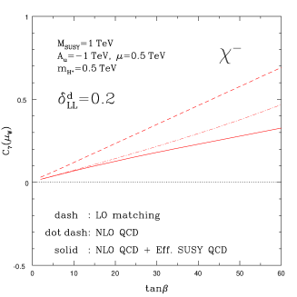
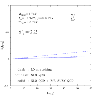
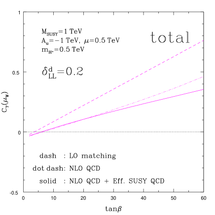
Figure 4: The Wilson coefficient $C_{7}({\mu}_{\rm W})$ vs. $\tan\beta$ for $M_{\rm SUSY}=1\,\mbox{TeV}$, $m_{\widetilde{g}}=\sqrt{2}\,m_{\widetilde{q}}=M_{\rm SUSY}$, $\mu=0.5\,\mbox{TeV}$, $A_{d}=0$, $A_{u}=-1\,\mbox{TeV}$, $m_{H^{+}}=0.5\,\mbox{TeV}$ and $\delta^{d}_{LL}=0.2$. All the other $\delta^{d,u}_{.~{}.}$’s are set to zero. In the upper left (right) window we show the chargino (gluino) contribution to $C_{7}({\mu}_{\rm W})$, and its total value from new physics in the main (lower) window. The dashed line shows the case of LO matching, the dot–dashed one includes the effect of NLO QCD, while the solid one includes also the effect of beyond–LO corrections from squark–gluino loops.

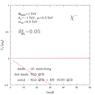
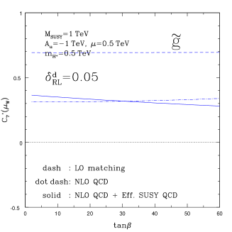
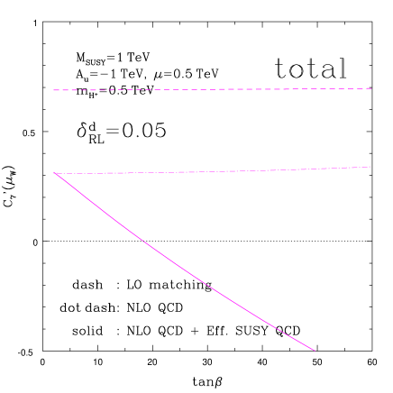
Figure 5: The Wilson coefficient $C_{7}^{\prime}({\mu}_{\rm W})$ vs. $\tan\beta$ for $\delta^{d}_{RL}=0.05$ and for the other parameters as in fig. 4.

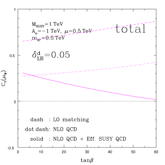
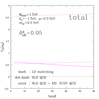
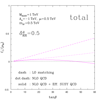
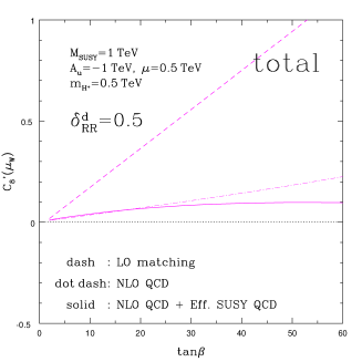
Figure 6: The Wilson coefficients $C_{7}({\mu}_{\rm W})$ (upper left) and $C_{8}({\mu}_{\rm W})$ (upper right) vs. $\tan\beta$ for $\delta^{d}_{RL}=0.05$; and $C_{7}^{\prime}({\mu}_{\rm W})$ (lower left) and $C_{8}^{\prime}({\mu}_{\rm W})$ (lower right) for $\delta^{d}_{RR}=0.5$. All other parameters as in fig. 4.

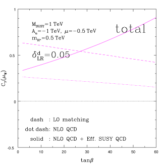
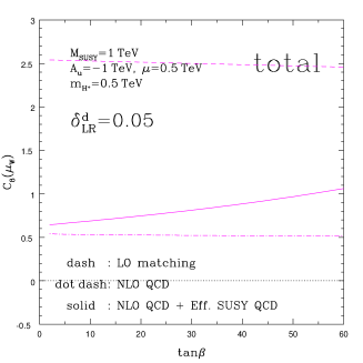
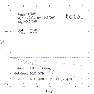
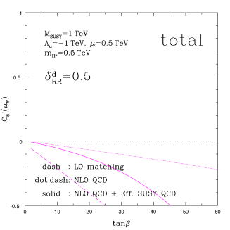
Figure 7: The same as in fig. 4 but for $\mu<0$.

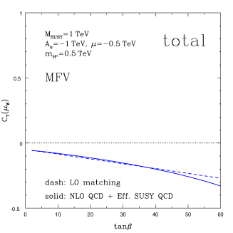
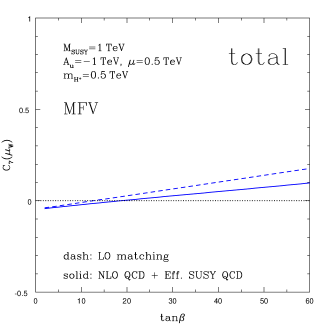
Figure 8: The coefficient $C_{7}({\mu}_{\rm W})$ vs. $\tan\beta$ in MFV for $\mu<0$ (left) and $\mu>0$ (right). All other parameters as in fig. 4. Relative to GFM, the difference between LO and beyond–LO effects is rather mild.

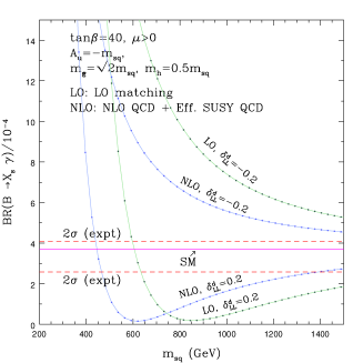
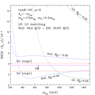
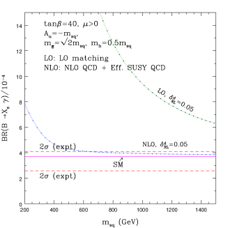
Figure 9: The branching ratio $BR(B\rightarrow X_{s}\gamma)/10^{-4}$ vs. $m_{\widetilde{q}}=m_{\rm sq}=M_{\rm SUSY}$ for in the LO and beyond–LO approximation for $\delta^{d}_{LL}=\pm 0.2$ (upper left), $\delta^{d}_{LR}=\pm 0.05$ (upper right), $\delta^{d}_{RL}=0.05$ (lower left) and $\delta^{d}_{RR}=0.5$ (lower right). All other parameters as in fig. 4.

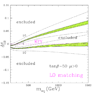
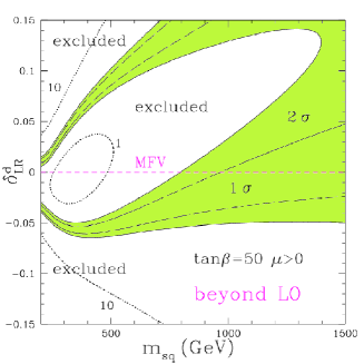
Figure 10: Contours of the branching ratio $BR(B\rightarrow X_{s}\gamma)/10^{-4}$ in the plane of $m_{\widetilde{q}}=m_{\rm sq}=M_{\rm SUSY}$ and $\delta^{d}_{LR}$ in LO approximation (left) and with dominant beyond–LO corrections included (right). Regions of the plane of $m_{\widetilde{q}}$ and $\delta^{d}_{LR}$ where the branching ratio $BR(B\rightarrow X_{s}\gamma)$ is consistent with experiment, eq. (1), at $1\sigma$ ($2\sigma$) are delineated with a long–dashed (solid) lines. We take $\tan\beta=50$, $m_{\widetilde{g}}=\sqrt{2}\,m_{\widetilde{q}}$, $A_{d}=0$, $A_{u}=-m_{\widetilde{q}}$, $\mu=0.5\,m_{\widetilde{q}}$, and $m_{H^{+}}=0.5\,m_{\widetilde{q}}$. The magenta short–dashed line marks the case of MFV. All the other $\delta^{d}$’s are set to zero.

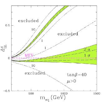
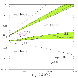
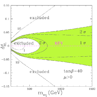
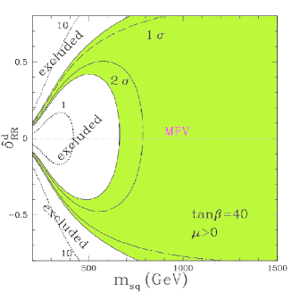
Figure 11: Contours of the branching ratio $BR(B\rightarrow X_{s}\gamma)/10^{-4}$ in the plane of $m_{\widetilde{q}}=m_{\rm sq}=M_{\rm SUSY}$ and $\delta^{d}_{LL}$ (upper left), $\delta^{d}_{LR}$ (upper right), $\delta^{d}_{RL}$ (lower left) and $\delta^{d}_{RR}$ (lower right) for $\tan\beta=40$ and $m_{\widetilde{g}}=m_{\widetilde{q}}$, $A_{d}=0$. All the other parameters are kept as in fig. 11. The long–dash (solid) curves delineate the regions which are consistent with experiment, eq. (1), at $1\sigma$ ($2\sigma$).

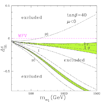
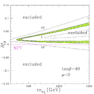
Figure 12: The same as in the upper two windows of fig. 11 but for $\mu<0$. In contrast, no ranges of $\delta^{d}_{RL}$ and $\delta^{d}_{RR}$ (lower two windows of fig. 11) are consistent with experiment.

5 Results

We will now demonstrate the effect of beyond–LO corrections to the Wilson coefficients derived above and to $BR(B\rightarrow X_{s}\gamma)$ with some representative examples. We will work in the super–CKM basis and in deriving our numerical examples will use the following parametrization: ${(m^{2}_{d,LL})}_{ii}=m^{2}_{\widetilde{q}}\,{\delta}_{ii}$, ${(m^{2}_{d,LL})}_{ij}=m^{2}_{\widetilde{q}}\,{(\delta^{d}_{LL})}_{ij}$ (and similarly for the $RR$ sector), ${(m^{2}_{d,LR})}_{ii}=A_{d}\,diag(m_{d},m_{s},m_{b})$ and ${(m^{2}_{d,LR})}_{ij}=m^{2}_{\widetilde{q}}\,{(\delta^{d}_{LR})}_{ij}=m^{2}_{\widetilde{q}}\,{(\delta^{d}_{RL})}^{\ast}_{ji}$, where $i,j=1,2,3$ and $i\neq j$. (Analogous parametrization is used also in the up–sector.) In the case of $b\rightarrow s\gamma$, the relevant mixings are those between the 2nd and 3rd generation squarks. For simplicity, in this section we will use the notation ${\delta^{d}_{{LL}}}=\left({\delta^{d}_{{LL}}}\right)_{23}$, etc. In all the cases presented in this section, we keep only one $\delta^{d,u}_{.~{}.}$ non–zero at a time and set all other $\delta^{d,u}_{.~{}.}$’s to zero.

First, we present the effect of including beyond–LO corrections derived in the previous sections. In the three panels of fig. 4 we plot the Wilson coefficient $C_{7}({\mu}_{\rm W})$ vs. $\tan\beta$ for $\delta^{d}_{LL}=0.2$, $\mu=500\,\mbox{GeV}$ and for other relevant parameters as specified in the figure caption. In particular, $A_{u}$ is chosen such that an approximate cancelation between the charged Higgs and the chargino contributions takes place in the case of $\mu>0$ for $\delta^{d}_{LL}=0$, similarly to the case of the Constrained MSSM (CMSSM). The dashed (solid) line corresponds to the LO (beyond–LO) value. (Here the LO matching is defined so that the SUSY contributions $\delta^{S}C_{7,8}$ are evaluated at ${\mu}_{\rm W}$, and the NLO corrections $\delta^{S}_{g,\widetilde{g}}C^{(1)}_{7,8}$ and $\delta^{W,H}_{\widetilde{g}}C^{(1)}_{7,8}$ are neglected.) The dash–dot line indicates the effect due to the NLO QCD correction only. Relative to the LO approximation, the chargino contribution, which in this case dominates $C_{7}({\mu}_{\rm W})$, is significantly reduced towards zero. As a result, the overall value of $C_{7}({\mu}_{\rm W})$ is also reduced, although, like in the LO case, it does grow with $\tan\beta$. (One finds a fairly similar effect for $C_{8}({\mu}_{\rm W})$ as well.)

Next, in fig. 5 we plot $C_{7}^{\prime}({\mu}_{\rm W})$ vs. $\tan\beta$ for $\delta^{d}_{RL}=0.05$, $\mu=500\,\mbox{GeV}$ and other parameters as in the previous figure. In this case, at LO the chargino contribution is zero while beyond–LO effects generate it on the negative side, with the magnitude growing with $\tan\beta$. In this sense, like before, the beyond–LO chargino contribution is again significantly reduced relative to the LO value. However, at some point it out–balances the gluino contribution which is also reduced but remains on the positive side and is roughly independent of $\tan\beta$. The total $C_{7}^{\prime}({\mu}_{\rm W})$ in this case decreases and at some point even changes sign. On the other hand, the total $C_{8}^{\prime}({\mu}_{\rm W})$ is reduced by a factor of about two but remains positive and roughly independent of $\tan\beta$. The main effect in $C_{8}^{\prime}({\mu}_{\rm W})$ comes from reducing the gluino part, while the chargino one is only slightly reduced down from zero.

Substantial beyond–LO effects also appear in the $LR$ and $RR$ sectors. In order to illustrate this, in the four panels of fig. 6 we plot $C_{7,8}({\mu}_{\rm W})$ and $C_{7,8}^{\prime}({\mu}_{\rm W})$ vs. $\tan\beta$ for $\delta^{d}_{LR}=0.05$ and $\delta^{d}_{RR}=0.5$, respectively. As a rule, $C_{8}({\mu}_{\rm W})$ and $C_{8}^{\prime}({\mu}_{\rm W})$, like in the previous cases, are reduced mostly because of a strong suppression of the gluino contribution. In all the cases of $C_{7,8}({\mu}_{\rm W})$ and $C_{7,8}^{\prime}({\mu}_{\rm W})$ presented in fig. 6, one finds that, in addition, the chargino contribution shifts from a positive, or zero, value down to an increasingly negative one, although much less so for $C_{8}({\mu}_{\rm W})$ than for $C_{7}({\mu}_{\rm W})$.

In the case of $\mu<0$, the two competing effects from the RG running and from the gluino–squark corrections lead to the NLO–corrected Wilson coefficients either decreasing or increasing with $\tan\beta$. This can be seen in the four panels of fig. 7 where all the other parameters are kept as before. In general, one can see that beyond–LO corrections to the Wilson coefficients are substantial. However, in contrast to the case of $\mu>0$, the Wilson coefficients can now either be larger or smaller relative to the LO approximation.

For comparison of the general GFM scenario with the limit of MFV, in fig. 8 we plot $C_{7}({\mu}_{\rm W})$ vs. $\tan\beta$ for the case of MFV and for $\mu=\pm 500\,\mbox{GeV}$ and the other parameters as before. The coefficient $C_{8}({\mu}_{\rm W})$ shows a similar behavior. It is clear that the effect of including beyond–LO corrections is not as striking as in GFM.

Large corrections to the Wilson coefficients in the case of GFM (but not MFV) often leads to substantial changes in the predictions for $BR(B\rightarrow X_{s}\gamma)$. In fact, the overall tendency is to reduce the magnitude of supersymmetric contributions relative to the LO, especially for large $\tan\beta$ and $\mu>0$. This leads to the “focusing effect” of concentrating on the SM value which we have identified in the previous paper [26]. We illustrated the effect in fig. 9 where we plot $BR(B\rightarrow X_{s}\gamma)$ vs. $m_{\widetilde{q}}$ for some typical choices of parameters. The focusing is indeed rather strong. In contrast, in the case of MFV the effect is much less pronounced [26].

As explained in ref. [26] and in sec. 1, focusing originates from two sources. Firstly, renormalization group evolution of $C_{7,8}$ from ${\mu}_{\rm SUSY}$ to ${\mu}_{\rm W}$ reduces the overall amplitude of these coefficients. In particular, the reduction of the strong coupling constant at ${\mu}_{\rm SUSY}$ has substantial effect on the gluino contribution. The NLO QCD matching at ${\mu}_{\rm SUSY}$ brings further suppression. Secondly, the gluino loop contribution to the mass matrix of down-type quark and the leading NLO SUSY–QCD corrections to the Wilson coefficients at ${\mu}_{\rm SUSY}$, $\delta^{\chi,\widetilde{g}}_{\widetilde{g}}C^{(\prime)(1)}_{7,8}$ have a common origin. This considerably reduces the LO gluino contribution to $C_{7,8}^{(\prime)}$, depending on the sign of $\mu$. At $\mu>0$ this correlation works as alignment, which is enhanced by $\tan\beta$ and explains the bulk of the focusing effect. For $\mu<0$, SUSY–QCD corrections cause anti–alignment instead, which competes with the overall suppression by renormalization group evolution and results in small focusing (or even de–focusing). Some NLO suppression of SUSY contribution already exits in MFV. However, flavor mixing is essential for the focusing effect with GFM as described above.

One important consequence of the focusing effect is a significant relaxation of bounds on the allowed amount of mixing in the squark sector relative to the LO approximation. We illustrate this in fig. 10 where we delineate the regions of the plane spanned by $\delta^{d}_{LR}$ and $m_{\widetilde{q}}$ where the predicted values of $BR(B\rightarrow X_{s}\gamma)$ are consistent with experiment, eq. (1), at $1\sigma$ (long–dashed) and $2\sigma$ (solid). One can see a significant enlargement of the allowed range of $\delta^{d}_{LR}$ relative to the LO approximation. Similar strong relaxation due to NLO–level corrections is also present for $\delta^{d}_{RL}$ and $\delta^{d}_{RR}$, and somewhat less so in the case of $\delta^{d}_{LL}$.

One should also note that, with even a small departure from the MFV case one can significantly weaken the lower bounds on $m_{\widetilde{q}}\sim M_{\rm SUSY}$ derived in the limit of MFV. The effect is already present in the LO approximation but it generally becomes further strengthened by including the beyond–LO corrections considered in this paper. It results mostly from a competition between the chargino and gluino contributions, the latter of which is in MFV absent.

The fact that lower limits on $M_{\rm SUSY}$ obtained in the case of MFV are highly unstable with respect to even small perturbations in the defining assumptions (40) of MFV, appears to be rather generic. To show this, in the four panels of fig. 11 we plot contours of $BR(B\rightarrow X_{s}\gamma)$ in the planes of $\delta^{d}_{.~{}.}$ and $m_{\widetilde{q}}$ for $\tan\beta=40$, $\mu>0$ and all the other parameters as specified in the figure caption. The bands delineated by dashed (solid) lines mark the $1\sigma$ ($2\sigma$) regions consistent with experiment (1). As before, only one $\delta^{d,u}_{.~{}.}$ is kept different from zero in each case. Note that in the regions in between the two allowed bands in the case of $\delta^{d}_{LL}$ and $\delta^{d}_{LR}$ the branching ratio reaches a shallow minimum whose position depends on the relative cancellation of the chargino and gluino contributions, and which also depends on $\tan\beta$ and other parameters. A similar shallow minimum appears in the case of small $\delta^{d}_{RL}$ or $\delta^{d}_{RR}$ and smaller $m_{\widetilde{q}}$. (It is worth noting that the values of $BR(B\rightarrow X_{s}\gamma)$ in the excluded region between the two bands is are such that a fair decrease of the experimental value would considerably reduce it.) Note that the cases of $\delta^{d}_{RL}$ and $\delta^{d}_{RR}$ the plots are almost symmetric. This is because of the new gluino contributions that appear in $C_{7,8}^{\prime}$ and which contribute to the branching ratio quadratically without interfering with the MFV contributions in $C_{7,8}$. In these cases, new contributions always come constructively. For $\mu<0$ (not shown in the figure) almost all of the region is excluded.

In the plots, $BR(B\rightarrow X_{s}\gamma)$ appears to be more sensitive to $\delta^{d}_{LR}$ and $\delta^{d}_{RL}$ than to $\delta^{d}_{LL}$ and $\delta^{d}_{RR}$ in our phenomenological approach. However, note that, once we assume a correlation between the A–terms and the Yukawa couplings, like in the MFV, the natural scale of $\delta^{d}_{LR}$ ($\delta^{d}_{RL}$) reduces from one to $m_{b}/M_{\rm SUSY}\mathrel{\hbox to0.0pt{\lower 4.0pt\hbox{\hskip 1.0pt$\sim$}\hss}\raise 1.0pt\hbox{$<$}}{\cal O}(10^{-2})$.

Even though the focusing effect considerably reduces the gluino contribution in the case of GFM, the branching ratio still shows strong dependence on $\delta^{d}_{LL}$ and $\delta^{d}_{LR}$ because of the interference between the gluino contributions and the MFV contributions to $C_{7,8}$. In addition, a new LO chargino contribution, other than the ones from the CKM mixing, is present in the $\delta^{d}_{LL}$ case because of the $SU(2)_{L}$ relation.

It is often claimed that the case of $\mu<0$ is inconsistent with ${BR(B\rightarrow X_{s}\gamma)}_{expt}$ (1). This is so because in the case of MFV the chargino contribution adds to the SM/2HDM contribution constructively for $\mu A_{u}>0$ and in unified models, like the CMSSM, with the boundary conditions $A_{0}=0$ (or similar), the RG running generates $A_{u}<0$ at $m_{\rm W}$. As a result, theoretical predictions are inconsistent with experiment, unless $M_{\rm SUSY}\mathrel{\hbox to0.0pt{\lower 4.0pt\hbox{\hskip 1.0pt$\sim$}\hss}\raise 1.0pt\hbox{$>$}}2\,\mbox{TeV}$, or so.

However, the claim is only true in the case of the strict MFV but not necessarily for even small departures from it, as can be seen in fig. 12. Indeed, for $\delta^{d}_{LL}\simeq-0.1$ and/or $\delta^{d}_{LR}\simeq-0.02$ one can even evade the bounds basically altogether. The effect is due to a partial cancellation of the chargino and gluino contributions which in the case of $\delta^{d}_{LL}$ can be efficient enough already in the LO approximation but in the case of $\delta^{d}_{LR}$ would only allow $m_{\widetilde{q}}$ down to some $500\,\mbox{GeV}$ but not lower. In contrast, beyond LO one can have $m_{\widetilde{q}}$ as small as some $200\,\mbox{GeV}$, as can be seen in fig. 12. On the other hand, for no ranges of $-0.15\leq\delta^{d}_{RL}\leq 0.15$ or $-0.8\leq\delta^{d}_{RR}\leq 0.8$ and $m_{\widetilde{q}}\leq 1.5\,\mbox{TeV}$ could we find any region consistent with experiment at either LO or beyond–LO level.

In tables 1–4 we present allowed ranges of the off–diagonal entries for a number of cases. As can be seen in figs. 10–12, typically there are two bands. In the cases of $\delta^{d}_{LL}$ and $\delta^{d}_{LR}$, one is around zero and one increasingly deviating from zero as $M_{\rm SUSY}$ increases. On the other hand, the allowed bands of $\delta^{d}_{RL}$ and $\delta^{d}_{RR}$ tend to be roughly symmetric, as mentioned above. As one can see from the tables, the allowed bands do not necessarily increase with $\tan\beta$. This is because the contributions from the chargino and the gluino show a different dependence on $\tan\beta$, and their approximate cancellation, can happen at different values of $\tan\beta$, as for example fig. 5 illustrates.

Table 1: Allowed range of $\delta^{d}_{LL}$ beyond LO, which resides within the $2\sigma$ experimental error. Parameters other than specified in the table are fixed to $M_{1}=M_{2}=m_{\widetilde{q}}$, $m_{h}=0.5m_{\widetilde{q}}$, $A_{u}=-m_{\widetilde{q}}$ and $A_{d}=0$.

$\delta^{d}_{LL}$ $(10^{-2})$
$\tan\beta$	$\mu>0$				$\mu<0$
$\,=40$	$m_{\widetilde{q}}=500{\rm GeV}$		$m_{\widetilde{q}}=1000{\rm GeV}$		$m_{\widetilde{q}}=500{\rm GeV}$		$m_{\widetilde{q}}=1000{\rm GeV}$
A	$(-6,-3)$,	$(21,23)$	$(-7,6)$,	$(74,77)$	$(-22,-20)$,	$(-9,-7)$	$(-50,-56)$,	$(-15,-8)$
B	$(-7,-4)$,	$(24,27)$	$(-8,7)$,	$(78,82)$	$(-25,-23)$,	$(-10,-8)$	$(-65,-61)$,	$(-17,-10)$
C	$(-4,\phantom{-}1)$,	$(26,29)$	$(-6,9)$,	$(82,86)$	$(-11,-10)$,	$(-5,-4)$	$(-38,-35)$,	$(-10,-6)$
D	$(-4,-2)$,	$(22,24)$	$(-2,10)$,	$(71,75)$	$(-23,-22)$,	$(-10,-9)$	$(-60,-56)$,	$(-20,-14)$
$\tan\beta$	$\mu>0$				$\mu<0$
$\,=60$	$m_{\widetilde{q}}=500{\rm GeV}$		$m_{\widetilde{q}}=1000{\rm GeV}$		$m_{\widetilde{q}}=500{\rm GeV}$		$m_{\widetilde{q}}=1000{\rm GeV}$
A	$(-7,-5)$,	$(13,15)$	$(-8,1)$,	$(59,61)$	$\simeq-13$,	$(-7,-6)$	$(-38,-36)$,	$(-11,-8)$
B	$(-8,-6)$,	$(15,18)$	$(-9,2)$,	$(64,69)$	$(-15,-14)$,	$(-8,-7)$	$(-42,-39)$,	$(-12,-9)$
C	$(-5,-3)$,	$(18,21)$	$(-7,4)$,	$(65,69)$	Not allowed		$(-14,-13)$,	$(-5,-4)$
D	$(-6,-4)$,	$(13,15)$	$(-5,3)$,	$(55,60)$	$(-14,-13)$,	$(-8,-7)$	$(-39,-36)$,	$(-14,-11)$

	$x_{\widetilde{g}}=(m_{\widetilde{g}}/m_{\widetilde{q}})^{2}$	$x_{\mu}=(|\mu|/m_{\widetilde{q}})^{2}$	$x_{H}=(m_{H}/m_{\widetilde{q}})^{2}$
Case A	1	0.25	0.25
Case B	2	0.25	0.25
Case C	1	1	0.25
Case D	1	0.25	0.04

Table 2: Allowed range of $\delta^{d}_{RR}$ with the same parameter set as in Table 1.

$\delta^{d}_{RR}$ $(10^{-2})$
	$\mu>0$			$\mu<0$
$\tan\beta=40$	$m_{\widetilde{q}}=500{\rm GeV}$		$m_{\widetilde{q}}=1000{\rm GeV}$	$m_{\widetilde{q}}=500{\rm GeV}$	$m_{\widetilde{q}}=1000{\rm GeV}$
A	$(-59,-41)$,	$(43,61)$	$(-90,93)$	Excluded	Excluded
B	$(-97,-93)$		No constraint	Excluded	Excluded
C	$(-30,-9)$,	$(11,31)$	$(-63,67)$	Excluded	Excluded
D	$(-50,-27)$,	$(28,51)$	$(-50,55)$	Excluded	Excluded
	$\mu>0$			$\mu<0$
$\tan\beta=60$	$m_{\widetilde{q}}=500{\rm GeV}$		$m_{\widetilde{q}}=1000{\rm GeV}$	$m_{\widetilde{q}}=500{\rm GeV}$	$m_{\widetilde{q}}=1000{\rm GeV}$
A	$(-71,-58)$,	$(59,72)$	No constraint	Excluded	Excluded
B	Excluded		No constraint	Excluded	Excluded
C	$(-28,-18)$,	$(19,29)$	$(-61,63)$	Not allowed	Excluded
D	$(-63,-50)$,	$(50,64)$	$(-78,81)$	Excluded	Excluded

Table 3: Allowed range of $\delta^{d}_{LR}$ with the same paramter set as in Table 1.

$\delta^{d}_{LR}$ $(10^{-2})$
	$\mu>0$				$\mu<0$
$\tan\beta=40$	$m_{\widetilde{q}}=500{\rm GeV}$		$m_{\widetilde{q}}=1000{\rm GeV}$		$m_{\widetilde{q}}=500{\rm GeV}$		$m_{\widetilde{q}}=1000{\rm GeV}$
A	$(-2,-1)$,	$(4,5)$	$(-1,1)$,	$\simeq 9$	$\simeq 1$,	$\simeq 3$	$\simeq 1$,	$(5,6)$
B	$(-4,-2)$,	$(8,9)$	$(-3,3)$,	$(17,20)$	$\simeq 2$,	$\simeq 4$	$(1,2)$,	$\simeq 7$
C	$(-1,\phantom{-}0)$,	$\simeq 5$	$(-1,1)$,	$(10,12)$	$\simeq 1$,	$\simeq 2$	$\simeq 1$,	$(4,5)$
D	$\simeq-1$,	$(4,5)$	$(0,2)$,	$(9,11)$	$\simeq 2$,	$\simeq 3$	$(1,2)$,	$(5,6)$
	$\mu>0$				$\mu<0$
$\tan\beta=60$	$m_{\widetilde{q}}=500{\rm GeV}$		$m_{\widetilde{q}}=1000{\rm GeV}$		$m_{\widetilde{q}}=500{\rm GeV}$		$m_{\widetilde{q}}=1000{\rm GeV}$
A	$(-3,-2)$,	$(4,5)$	$(-2,1)$,	$(10,13)$	$\simeq 2$,	$\simeq 3$	$\simeq 1$,	$(4,5)$
B	$(-10,-7)$,	$(8,10)$	$(-11,17)$		$\simeq 2$,	$\simeq 4$	$(1,2)$,	$\simeq 6$
C	$(-2,-1)$,	$(5,6)$	$(-2,1)$,	$(12,15)$	Not allowed		$\simeq 1$,	$\simeq 3$
D	$(-3,-2)$,	$(4,5)$	$(-2,1)$,	$(10,13)$	$\simeq 2$,	$\simeq 3$	$\simeq 2$,	$\simeq 5$

Table 4: Allowed range of $\delta^{d}_{RL}$ with the same parameter set as in Table 1.

$\delta^{d}_{RL}$ $(10^{-2})$
	$\mu>0$			$\mu<0$
$\tan\beta=40$	$m_{\widetilde{q}}=500{\rm GeV}$		$m_{\widetilde{q}}=1000{\rm GeV}$	$m_{\widetilde{q}}=500{\rm GeV}$	$m_{\widetilde{q}}=1000{\rm GeV}$
A	$(-5,-3)$,	$(3,4)$	$(-6,6)$	Excluded	Excluded
B	$(-5,-3)$,	$(3,5)$	$(-6,5)$	Excluded	Excluded
C	$(-4,-1)$,	$(1,4)$	$(-6,6)$	Excluded	Excluded
D	$(-4,-2)$,	$(2,4)$	$(-4,3)$	Excluded	Excluded
	$\mu>0$			$\mu<0$
$\tan\beta=60$	$m_{\widetilde{q}}=500{\rm GeV}$		$m_{\widetilde{q}}=1000{\rm GeV}$	$m_{\widetilde{q}}=500{\rm GeV}$	$m_{\widetilde{q}}=1000{\rm GeV}$
A	$(-4,-3)$,	$(3,4)$	$(-5,5)$	Excluded	Excluded
B	$(-3,-2)$,	$(2,3)$	$(-4,3)$	Excluded	Excluded
C	$(-7,\phantom{-}4)$,	$(4,7)$	$(-10,10)$	Not allowed	Excluded
D	$(-4,-3)$,	$(3,4)$	$(-4,4)$	Excluded	Excluded

Figure 13: Contours of the ratio $K^{(0)}_{cb}/K_{cb}$ in the plane spanned by $m_{\widetilde{q}}=m_{\rm sq}$ and $\delta^{d}_{LR}$. We fix $m_{\widetilde{g}}=\sqrt{2}\,m_{\widetilde{q}}$, $A_{d}=0$, $A_{u}=-m_{\widetilde{q}}$, $\mu=0.5\,m_{\widetilde{q}}$, and $m_{H^{+}}=0.5\,m_{\widetilde{q}}$ and show two cases $\tan\beta=40$ (left) and $\tan\beta=60$ (right).

The significant enlargement of the allowed parameter space in the framework of GFM, relative to MFV, leads to a strong relaxation of constraints on the allowed ranges of the “bare” CKM matrix element $K^{(0)}_{cb}$ relative to $K_{cb}\simeq 0.04$ which is determined by experiment. In the two windows of fig. 13 we present contours of the ratio $K^{(0)}_{cb}/K_{cb}$ in the plane spanned by $m_{\widetilde{q}}=m_{\rm sq}=M_{\rm SUSY}$ and $\delta^{d}_{LR}$. We fix $m_{\widetilde{g}}=\sqrt{2}\,m_{\widetilde{q}}$, $A_{d}=0$, $A_{u}=-m_{\widetilde{q}}$, $\mu=0.5\,m_{\widetilde{q}}$, and $m_{H^{+}}=0.5\,m_{\widetilde{q}}$ and show two cases $\tan\beta=40$ (left) and $\tan\beta=60$ (right). One can see that the ratio $K^{(0)}_{cb}/K_{cb}$ can exceed a factor of ten, or more, for large enough, but still allowed, ranges of $\delta^{d}_{LR}$. It is also interesting that the ratio can be much smaller than one and that it can even “cross” zero in the allowed region between the two contours of 1. In this case the measured value of $K^{(0)}_{cb}$ is of purely radiative origin and is generated by GFM in supersymmetry [29]. On the other hand, for large $\delta^{d}_{LL}\mathrel{\hbox to0.0pt{\lower 4.0pt\hbox{\hskip 1.0pt$\sim$}\hss}\raise 1.0pt\hbox{$<$}}0.8$ the ratio does not exceed a factor of three.

6 Conclusions

The squark–gluino loop correction that appears beyond the LO in the inclusive process $b\rightarrow s\gamma$ shows a large effect in the MSSM with general flavor mixing. Its main feature is that of reducing the magnitude of supersymmetric (mostly gluino) contribution to $BR(B\rightarrow X_{s}\gamma)$ relative to the LO approximation. This focusing effect leads to a considerable relaxation of experimental constraints on flavor mixing terms and on the lower bounds on $M_{\rm SUSY}$ obtained in the limit of MFV, to the extent of even allowing small $M_{\rm SUSY}$ at $\mu<0$.

Given such a large effect appearing beyond LO, one may question the validity of perturbation theory in the analysis presented here. However, in this case the mechanism that generates it, namely the large gluino–squark corrections, is absent at LO. We believe that the mechanism is a dominant one at NLO, although we have examined it within the limitations of our assumptions. It would therefore be highly desirable to have available a complete NLO calculation of $BR(B\rightarrow X_{s}\gamma)$ in supersymmetry with GFM which would be applicable in more general circumstances than those considered here. It is also clear that, with improving experimental precision, an NLO-level analysis appears to be essential in testing SUSY models of flavor at large $\tan\beta$, like, for example, those based on a SO(10) SUSY GUT [46].

Appendix A Effective $W^{\pm}$ and $H^{\pm}$ Vertices

In this Appendix we summarize the effective vertices of $W^{\pm}$–boson (unphysical scalar $G^{\pm}$) and charged Higgs boson $H^{\pm}$ which arise from integrating out gluino–squark loops at the matching scale $\mu_{SUSY}$. All the coupling constants and masses appearing in the following are evaluated in the effective SM at some arbitrary scale $\mu$ although in actual expressions for Wilson coefficients they will be evaluated at the scale $\mu_{SUSY}$. We work in the $\overline{MS}$–scheme except for the case explicitly mentioned. The renormalization group equations for evolving the couplings in the effective SM to $\mu_{SUSY}$ from their values at $\mu_{W}$ are given in [44]. We work in the physical super–CKM basis where the loop–corrected mass matrices $m_{{d,u}}$  (5)–(6) of both the down– and up–type quarks are diagonal.

A.1 $W^{\pm}$–boson

The effective $u\,d\,W$ vertex, evaluated at some scale $\mu$, is given by

$${\cal L} = -\frac{g_{2}}{\sqrt{2}}\sum^{3}_{i,j=1}\overline{u}_{i}(\mu)\gamma^{\mu}W_{\mu}P_{L}K^{\rm eff}_{ij}d_{j}+h.c.$$ (65)

Note the effective CKM matrix $K^{\rm eff}_{ij}$ which appears in (65), instead of $K_{ij}$ ($i,j=1,2,3$)

$$K^{\rm eff}_{ij} = K_{ij}+\left(\frac{\alpha_{s}}{4\pi}\right)\Delta K_{ij},$$ (67)

where

$$\Delta K_{ij} = 4C_{2}(3)\sum^{3}_{k,l=1}\sum^{6}_{I,J=1}{(\Gamma_{u\,L}^{\ast})}_{Ii}{(\Gamma_{u\,L})}_{Ik}K_{kl}{(\Gamma_{d\,L}^{\ast})}_{Jl}{(\Gamma_{d\,L})}_{Jj}C_{24}(m_{\widetilde{g}}^{2},{m_{\widetilde{u}_{I}}^{2}},{m_{\widetilde{d}_{J}}^{2}};\mu)$$ (68)

$$+\frac{1}{2}\sum^{3}_{k=1}\left[{(\Delta Z_{u\,L}^{\ast})}_{ki}K_{kj}+K_{ik}{(\Delta Z_{d\,L})}_{kj}\right].$$

The first term above is due to the $W$–boson coupling to the intermediate squark fields, while in the remaining two the $W$–boson couples to the external quark lines, and

$$(\Delta Z_{u\,L})_{ij}(\mu) = 2C_{2}(3)\sum^{6}_{I=1}{(\Gamma_{u\,L}^{\ast})}_{Ii}(\Gamma_{u\,L})_{Ij}B_{1}(m_{\widetilde{g}}^{2},m_{\widetilde{u}_{I}}^{2},0;\mu),$$ (69)

$$(\Delta Z_{d\,L})_{ij}(\mu) = 2C_{2}(3)\sum^{6}_{I=1}{(\Gamma_{d\,L}^{\ast})}_{Ii}{(\Gamma_{d\,L})}_{Ij}B_{1}(m_{\widetilde{g}}^{2},m_{\widetilde{d}_{J}}^{2},0;\mu).$$ (70)

It is the elements $K^{\rm eff}_{ij}$ that are equal to the experimentally determined elements of the CKM matrix. The elements of $K_{ij}$ are then determined by (67) but the difference with $K^{\rm eff}_{ij}$ is rather tiny.

Note that the effective vertex defined by (65) gives finite contributions since $\ln\mu$ and infinite terms which appear in the Passarino–Veltman functions, which are collected in appendix C, disappear in actual calculations.

A.2 Unphysical scalar $G^{\pm}$

The effective vertices of the unphysical scalar $G^{\pm}$ with $d$ and $u$, evaluated at the scale $\mu_{W}$ in the ’t Hooft–Feynman gauge, are given by

$${\cal L} = \sum^{3}_{i,j=1}\overline{u}_{i}\left(C^{Gu_{i}d_{j}}_{L}P_{L}+C^{Gu_{i}d_{j}}_{R}P_{R}\right)G^{+}d_{j}+h.c.,$$ (71)

where the couplings $C^{Gu_{i}d_{j}}_{L,R}$ receive contributions from the tree–level $C^{Gu_{i}d_{j}(0)}_{L,R}$ and from squark–gluino loops $C^{Gu_{i}d_{j}(1)}_{L,R}$

$$C^{Gu_{i}d_{j}}_{L,R} = C^{Gu_{i}d_{j}(0)}_{L,R}+\frac{\alpha_{s}(\mu_{W})}{4\pi}C^{Gu_{i}d_{j}(1)}_{L,R}.$$ (72)

The former are given by

$$C^{Gu_{i}d_{j}(0)}_{L}=\frac{g_{2}{\overline{m}_{u}}_{i}({\mu}_{\rm W})K_{ij}}{\sqrt{2}m_{W}},~{}~{}~{}~{}~{}~{}~{}~{}~{}~{}~{}~{}~{}~{}C^{Gu_{i}d_{j}(0)}_{R}=-\frac{g_{2}K_{ij}{\overline{m}_{d}}_{j}({\mu}_{\rm W})}{\sqrt{2}m_{W}},$$ (73)

where ${\overline{m}_{u}}_{j}({\mu}_{\rm W})$ and ${\overline{m}_{d}}_{j}({\mu}_{\rm W})$ denote the running quark masses at $\mu_{W}$. For simplicity we have neglected here a small rotation of the quark mass basis due to the renormalization group evolution between ${\mu}_{\rm W}$ and ${\mu}_{\rm SUSY}$.

The corrections are given by

$$C^{Gu_{i}d_{j}(1)}_{L} = \eta^{\frac{3}{7}}\left[-2C_{2}(3)\sum^{6}_{I,J=1}{(\Gamma_{u\,R}^{\ast})}_{Ii}{(\Gamma_{d\,L})}_{Jj}\left(C^{G\widetilde{d}_{J}\widetilde{u}_{I}}\right)^{\ast}m_{\widetilde{g}}C_{0}(m_{\widetilde{u}_{I}}^{2},m_{\widetilde{d}_{J}}^{2},m_{\widetilde{g}}^{2})\right.$$ (74)

$$\phantom{eta^{\frac{3}{7}}}\left.-\frac{g_{2}}{\sqrt{2}m_{W}}\sum_{k=1}^{3}{(\delta{m_{u}})}_{ik}K_{kj}\right.$$

$$\phantom{eta^{\frac{3}{7}}}\left.+\frac{1}{2}\sum^{3}_{k,l,m=1}C^{Gu_{i}d_{k}(0)}_{L}\left[(\Delta Z_{d\,L})_{kj}-K^{\ast}_{lk}{(\Delta Z_{u\,L})}_{lm}K_{mj}\right]\right],$$

$$C^{Gu_{i}d_{j}(1)}_{R} = \eta^{\frac{3}{7}}\left[2C_{2}(3)\sum^{6}_{I,J=1}{(\Gamma_{u\,L}^{\ast})}_{Ii}{(\Gamma_{d\,R})}_{Jj}\left(C^{G\widetilde{d}_{J}\widetilde{u}_{I}}\right)^{\ast}m_{\widetilde{g}}C_{0}(m_{\widetilde{u}_{I}}^{2},m_{\widetilde{d}_{J}}^{2},m_{\widetilde{g}}^{2})\right.$$ (75)

$$\phantom{eta^{\frac{3}{7}}}\left.+\frac{g_{2}}{\sqrt{2}m_{W}}\sum_{k=1}^{3}K_{ik}{(\delta{m_{d}^{\ast}})}_{jk}\right.$$

$$\phantom{eta^{\frac{3}{7}}}\left.-\frac{1}{2}\sum^{3}_{k,l,m=1}\left[(\Delta Z_{u\,L}^{\ast})_{ki}-K_{il}(\Delta Z_{d\,L}^{\ast})_{ml}K^{\ast}_{km}\right]C^{Gu_{k}d_{j}(0)}_{R}\right],$$

where $C_{0}$ is a Passarino–Veltman function and the expressions for $(\delta m_{d,u})_{ik}$ are given in and below eq. (32).

The factor $\eta=\alpha_{s}({\mu}_{\rm SUSY})/\alpha_{s}({\mu}_{\rm W})$ appears as the result of running the couplings $C^{Gu_{i}d_{j}(1)}_{L,R}$, which are initially evaluated at ${\mu}_{\rm SUSY}$, down to ${\mu}_{\rm W}$, with the SM QCD RGE’s including six quark flavors.

The functions $\Delta Z_{u\,L}$ and $\Delta Z_{d\,L}$ are defined in (69) and (70), and

$$C^{G\widetilde{d}_{I}\widetilde{u}_{J}} = -\frac{g_{2}}{\sqrt{2}m_{W}}\sum^{3}_{k,l,m=1}{(\Gamma_{d\,R})}_{Ik}\left[{(m^{2\ast}_{d,LR})}_{lk}-m_{d_{k}}\mu^{\ast}\tan\beta\,\delta_{kl}\right]K^{\ast}_{ml}{(\Gamma_{u\,L}^{\ast})}_{Jm}$$ (76)

$$+\frac{g_{2}}{\sqrt{2}m_{W}}\sum^{3}_{k,l,m=1}{(\Gamma_{d\,L})}_{Ik}K^{\ast}_{lk}\left[{(m^{2}_{u,LR})}_{lm}-m_{u_{l}}\mu\cot\beta\,\delta_{lm}\right]{(\Gamma_{u\,R}^{\ast})}_{Jm}.$$

Like in the case of the effective coupling of the $W$–boson above, $\ln\mu$ and infinite terms in $B_{0}$ effectively do not contribute because of the unitarity of the diagonalization matrices $\Gamma$.

A.3 Charged Higgs boson $H^{\pm}$

The effective $H^{\pm}$ vertices with $d$ and $u$, evaluated at the ${\mu}_{\rm W}$, are given by

$${\cal L} = \sum^{3}_{i,j=1}\overline{u}_{i}\left(C^{Hu_{i}d_{j}}_{L}P_{L}+C^{Hu_{i}d_{j}}_{R}P_{R}\right)H^{+}d_{j}+h.c.,$$ (77)

where, similarly to the case of the unphysical scalar before, the couplings $C^{Hu_{i}d_{j}L,R}$ receive contributions from the tree–level $C^{Hu_{i}d_{j}(0)}_{L,R}$ and from squark–gluino loops $C^{Hu_{i}d_{j}(1)}_{L,R}$

$$C^{Hu_{i}d_{j}}_{L,R} = C^{Hu_{i}d_{j}(0)}_{L,R}+\frac{\alpha_{s}(\mu_{W})}{4\pi}C^{Hu_{i}d_{j}(1)}_{L,R}.$$ (78)

The former are given by

$$C^{Hu_{i}d_{j}(0)}_{L}=\frac{g_{2}{\overline{m}_{u}}_{i}K_{ij}}{\sqrt{2}m_{W}}\cot\beta,~{}~{}~{}~{}~{}~{}~{}~{}~{}~{}~{}~{}~{}~{}C^{Hu_{i}d_{j}(0)}_{R}=\frac{g_{2}K_{ij}{\overline{m}_{d}}_{j}}{\sqrt{2}m_{W}}\tan\beta,$$ (79)

where ${\overline{m}_{u}}_{i}$ and ${\overline{m}_{d}}_{i}$ have been defined below eq. (73). The corrections are given by

$$C^{Hu_{i}d_{j}(1)}_{L} = \eta^{\frac{3}{7}}\left[2C_{2}(3)\sum^{6}_{I,J=1}{(\Gamma_{u\,R}^{\ast})}_{Ii}{(\Gamma_{d\,L})}_{Jj}\left(C^{H\widetilde{d}_{J}\widetilde{u}_{I}}\right)^{\ast}m_{\widetilde{g}}C_{0}(m_{\widetilde{u}_{I}}^{2},m_{\widetilde{d}_{J}}^{2},m_{\widetilde{g}}^{2})\right.$$ (80)

$$\phantom{\eta^{\frac{3}{7}}}\left.+\frac{g_{2}\cot\beta}{\sqrt{2}m_{W}}\sum_{k=1}^{3}{(\Delta{m_{u}})}_{ik}K_{kj}\right.$$

$$\phantom{\eta^{\frac{3}{7}}}\left.+\frac{1}{2}\sum^{3}_{k,l,m=1}C^{Hu_{i}d_{k}(0)}_{L}\{(\Delta Z_{d\,L})_{kj}-K^{\ast}_{lk}(\Delta Z_{u\,L})_{lm}K_{mj}\}\right],$$

$$C^{Hu_{i}d_{j}(1)}_{R} = \eta^{\frac{3}{7}}\left[-2C_{2}(3)\sum^{6}_{I,J=1}{(\Gamma_{u\,L}^{\ast})}_{Ii}{(\Gamma_{d\,R})}_{Jj}\left(C^{H\widetilde{d}_{J}\widetilde{u}_{I}}\right)^{\ast}m_{\widetilde{g}}C_{0}(m_{\widetilde{u}_{I}}^{2},m_{\widetilde{d}_{J}}^{2},m_{\widetilde{g}}^{2})\right.$$ (81)

$$\phantom{\eta^{\frac{3}{7}}}\left.+\frac{g_{2}\tan\beta}{\sqrt{2}m_{W}}\sum_{k=1}^{3}K_{ik}{(\Delta{{m_{d}}^{\ast}})}_{jk}\right.$$

$$\phantom{\eta^{\frac{3}{7}}}\left.-\frac{1}{2}\sum^{3}_{k,l,m=1}\{(\Delta Z_{u\,L}^{\ast})_{ki}-K_{il}(\Delta Z_{d\,L}^{\ast})_{ml}K^{\ast}_{km}\}C^{Hu_{k}d_{j}(0)}_{R}\right],$$

As in the previous subsection, the factor $\eta$ appears as the result of running the couplings $C^{Hu_{i}d_{j}(1)}_{L,R}$, which are initially evaluated at ${\mu}_{\rm SUSY}$, down to ${\mu}_{\rm W}$, with SM QCD RGE’s assuming six flavors.

$$C^{H\widetilde{d}_{I}\widetilde{u}_{J}} = \frac{g_{2}}{\sqrt{2}m_{W}}\sum^{3}_{k,l,m=1}{(\Gamma_{d\,R})}_{Ik}\left[{(m^{2\ast}_{d,LR})}_{lk}\tan\beta-\mu^{\ast}{m_{d_{k}}}\delta_{kl}\right]K^{\ast}_{ml}{(\Gamma_{u\,L}^{\ast})}_{Jm}$$ (82)

$$+\frac{g_{2}}{\sqrt{2}m_{W}}\sum^{3}_{k,l,m=1}{(\Gamma_{d\,L})}_{Ik}K^{\ast}_{lk}\left[{(m^{2}_{u,LR})}_{lm}\cot\beta-\mu{m_{u_{l}}}\delta_{lm}\right]{(\Gamma_{u\,R}^{\ast})}_{Jl}.$$

Appendix B Effective $\chi^{\pm}$, $\chi^{0}$ and $\widetilde{g}$ Vertices

We summarize here the effective vertices of the chargino $\chi^{\pm}$, neutralino $\chi^{0}$ and gluino $\widetilde{g}$ fields, evaluated at ${\mu}_{\rm SUSY}$. Notice that the corrections to the tree–level vertices come as a result of using gluino–squark loop–corrected values for the quark and squark quantities appearing in the expressions below.

B.1 Chargino $\chi^{\pm}$

The effective quark–squark–chargino vertices are given by

$${\cal L} = \sum^{3}_{i=1}\sum^{2}_{a=1}\sum^{6}_{I=1}\overline{d}_{i}\left[{(C_{d\,L})}_{iaI}P_{L}+{(C_{d\,R})}_{iaI}P_{R}\right]\chi^{-}_{a}\widetilde{u}_{I}+h.c.,$$ (83)

where

$${(C_{d\,L})}_{iaI} = \frac{g_{2}}{\sqrt{2}m_{W}}\sum^{3}_{k=1}\frac{{(m_{d}^{(0)})}_{ik}}{\cos\beta}U_{a2}{(\Gamma_{u\,L}^{\ast})}_{Ik},$$ (84)

$${(C_{d\,R})}_{iaI} = -g_{2}V_{a1}{(\Gamma_{u\,L}^{\ast})}_{Ii}+\frac{g_{2}}{\sqrt{2}m_{W}}\sum^{3}_{k=1}\frac{{(m_{u}^{(0)\ast})}_{ki}}{\sin\beta}V_{a2}{(\Gamma_{u\,R}^{\ast})}_{Ik},$$ (85)

and $V$ and $U$ are the $2\times 2$ two matrices with which one diagonalizes the chargino mass matrix.

B.2 Neutralino $\chi^{0}$

The corrected quark–squark–neutralino vertices are given by

$${\cal L} = \sum^{3}_{i=1}\sum^{4}_{r=1}\sum^{6}_{I=1}\overline{d}_{i}\left[(N_{d\,L})_{irI}P_{L}+(N_{d\,R})_{irI}P_{R}\right]\chi^{0}_{r}\widetilde{d}_{I}+h.c.,$$ (86)

where

$$(N_{d\,L})_{irI} = -\sqrt{2}g_{2}\left[\frac{1}{3}\tan\theta_{W}N_{r1}^{\ast}{(\Gamma_{d\,R}^{\ast})}_{Ii}+\frac{(m^{(0)}_{d})_{ik}}{2m_{W}\cos\beta}N_{r3}^{\ast}{(\Gamma_{d\,L}^{\ast})}_{Ik}\right],$$ (87)

$$(N_{d\,R})_{irI} = -\sqrt{2}g_{2}\left[\left(-\frac{1}{2}N_{r2}+\frac{1}{6}\tan\theta_{W}N_{r11}\right){(\Gamma_{d\,L}^{\ast})}_{Ii}\right.$$ (88)

$$\left.\phantom{-\sqrt{2}g_{2}[}+\frac{(m^{(0)\ast}_{d})_{ki}}{2m_{W}\cos\beta}N_{r3}{(\Gamma_{d\,R}^{\ast})}_{Ik}\right],$$

and $N$ is the $4\times 4$ matrix with which one diagonalizes the neutralino mass matrix [34].

B.3 Gluino $\widetilde{g}$

The effective quark–squark–gluino vertices are given by

$${\cal L} = \sum^{3}_{i=1}\sum^{6}_{I=1}\overline{d}_{i}\left[{(G_{d\,L})}_{iI}P_{L}+{(G_{d\,R})}_{iI}P_{R}\right]\widetilde{d}_{I}\widetilde{g}$$ (89)

$$+ \sum^{3}_{i=1}\sum^{6}_{I=1}\overline{u}_{i}\left[{(G_{u\,L})}_{iI}P_{L}+{(G_{u\,R})}_{iI}P_{R}\right]\widetilde{u}_{I}\widetilde{g}+h.c.,$$

where

$${(G_{dL})}_{iI}=-\sqrt{2}g_{s}{(\Gamma_{dR}^{\ast})}_{Ii},~{}~{}~{}~{}~{}~{}~{}{(G_{dR})}_{iI}=\sqrt{2}g_{s}{(\Gamma_{dL}^{\ast})}_{Ii},$$ (90)

and analogously for the up–type sector.

The above effective couplings for the chargino, neutralino and gluino reduce to their tree–level values by making the following replacements: $\left(\Gamma_{du\,LR}\right)_{Ii}\rightarrow\left(\Gamma_{du\,LR}^{(0)}\right)_{Ii}$ and $\left(m^{(0)}_{d,u}\right)_{ij}\rightarrow\left(m_{d,u}\right)_{ij}\delta_{ij}$.

Appendix C Passarino-Veltman functions

We present here explicit expressions for the Passarino-Veltman functions [45] which appear in our calculation. We take all the external momenta equal to zero.

$$B_{0}(x,y;\mu) = \frac{1}{\epsilon}+2\ln{\mu}-1-\frac{x\ln{x}-y\ln{y}}{x-y},$$ (91)

$$B_{1}(x,y;\mu) = -\frac{1}{2}\frac{1}{\epsilon}-\ln{\mu}-\frac{1}{4}\frac{3x-y}{x-y}$$ (92)

$$+\frac{x^{2}}{(x-y)^{2}}\ln{x}-\frac{1}{2}\frac{(2x-y)y}{(x-y)^{2}}\ln{y},$$

$$C_{0}(x,y,z) = -\left\{\frac{x\ln{x}}{(y-x)(z-x)}\right.$$ (93)

$$\left.+\frac{y\ln{y}}{(z-y)(x-y)}+\frac{z\ln{z}}{(x-z)(y-z)}\right\},$$

$$C_{24}(x,y,z;\mu) = \frac{1}{4}\left\{\frac{1}{\epsilon}+2\ln{\mu}+\frac{3}{2}\right.-\frac{x^{2}\ln{x}}{(x-y)(x-z)}$$ (94)

$$\left.-\frac{y^{2}\ln{y}}{(y-x)(y-z)}-\frac{z^{2}\ln{z}}{(z-x)(z-y)}\right\}.$$

Appendix D Mass functions for the Wilson coefficients

In this section we collect several auxiliary functions which appear in sec. 4. The mass functions for the SM and 2HDM contributions to $C_{7,8}$ are given in [8],

$$F_{7}^{(1)}(x)= \frac{x(7-5x-8x^{2})}{24(x-1)^{3}}+\frac{x^{2}(3x-2)}{4(x-1)^{4}}\ln x,$$ (95)

$$F_{8}^{(1)}(x)= \frac{x(2+5x-x^{2})}{8(x-1)^{3}}-\frac{3x^{2}}{4(x-1)^{4}}\ln x,$$ (96)

$$F_{7}^{(2)}(x)= \frac{x(3-5x)}{12(x-1)^{2}}+\frac{x(3x-2)}{6(x-1)^{3}}\ln x,$$ (97)

$$F_{8}^{(2)}(x)= \frac{x(3-x)}{4(x-1)^{2}}-\frac{x}{2(x-1)^{3}}\ln x.$$ (98)

The mass functions and related constants for the $\chi^{-}$, $\chi^{0}$ and $\widetilde{g}$ contributions to $C_{7,8}$ are given in [41],

$$H^{[7]}_{1}(x)= \frac{-3x^{2}+2x}{6(1-x)^{4}}\ln x+\frac{-8x^{2}-5x+7}{36(1-x)^{3}},$$ (99)

$$H^{[8]}_{1}(x)= \frac{x}{2(1-x)^{4}}\ln x+\frac{-x^{2}+5x+2}{12(1-x)^{3}},$$ (100)

$$H^{[7]}_{2}(x)= \frac{-3x^{2}+2x}{3(1-x)^{3}}\ln x+\frac{-5x^{2}+3x}{6(1-x)^{2}},$$ (101)

$$H^{[8]}_{2}(x)= \frac{x}{(1-x)^{3}}\ln x+\frac{-x^{2}+3x}{2(1-x)^{2}},$$ (102)

$$H^{[7]}_{3}(x)= -\frac{1}{3}H^{[8]}_{1}(x),$$ (103)

$$H^{[8]}_{3}(x)= H^{[8]}_{1}(x),$$ (104)

$$H^{[7]}_{4}(x)= -\frac{1}{3}\left(H^{[8]}_{2}(x)+\frac{1}{2}\right),$$ (105)

$$H^{[8]}_{4}(x)= H^{[8]}_{2}(x)+\frac{1}{2},$$ (106)

$$H^{[7]}_{5}(x)= -\frac{1}{3}H^{[8]}_{1}(x),$$ (107)

$$H^{[8]}_{5}(x)= \frac{9x^{2}-x}{16(1-x)^{4}}\ln x+\frac{19x^{2}+40x-11}{96(1-x)^{3}},$$ (108)

$$H^{[7]}_{6}(x)= -\frac{1}{3}\left(H^{[8]}_{2}(x)+\frac{1}{2}\right),$$ (109)

$$H^{[8]}_{6}(x)= \frac{9x^{2}-x}{8(1-x)^{3}}\ln x+\frac{13x-5}{8(1-x)^{2}},$$ (110)

$$\lambda^{[7]}= \frac{5}{6},~{}~{}~{}~{}~{}\lambda^{[8]}=\frac{1}{2}.$$ (111)

Appendix E NLO QCD corrections to the Wilson coefficients

For completeness, in this section we collect the NLO QCD corrections to the Wilson coefficients given in [8, 41].

The NLO QCD corrections to the Wilson coefficients in the SM are summarized as [8],

$$\delta^{W}_{g}C_{i}^{(1)}({\mu}_{\rm W})=\begin{cases}15+6\ln\frac{{\mu}_{\rm W}^{2}}{m_{W}^{2}},&\text{for}~{}~{}~{}i=1,\\ 0,&\text{for}~{}~{}~{}i=2,3,5,6,\\ E\left(\frac{\overline{m}_{t}^{2}({\mu}_{\rm W})}{m_{W}^{2}}\right)-\frac{2}{3}+\frac{2}{3}\ln\frac{{\mu}_{\rm W}^{2}}{m_{W}^{2}},&\text{for}~{}~{}~{}i=4,\\ G_{i}\left(\frac{\overline{m}_{t}^{2}({\mu}_{\rm W})}{m_{W}^{2}}\right)+\Delta_{i}\left(\frac{\overline{m}_{t}^{2}({\mu}_{\rm W})}{m_{W}^{2}}\right)\ln\frac{{\mu}_{\rm W}^{2}}{m_{W}^{2}},&\text{for}~{}~{}~{}i=7,8,\end{cases}$$ (112)

where

$$\begin{split}E(x)=&\frac{x(-18+11x+x^{2})}{12(x-1)^{3}}+\frac{x^{2}(15-16x+4x^{2})}{6(x-1)^{4}}\ln x-\frac{2}{3}\ln x,\end{split}$$ (113)

$$\begin{split}G_{7}(x)=&\frac{-16x^{4}-122x^{3}+80x^{2}-8x}{9(x-1)^{4}}{\rm Li_{2}}\left(1-\frac{1}{x}\right)\\ &+\frac{6x^{4}+46x^{3}-28x^{2}}{3(x-1)^{5}}\ln^{2}x\\ &+\frac{-102x^{5}-588x^{4}-2262x^{3}+3244x^{2}-1364x+208}{81(x-1)^{5}}\ln x\\ &+\frac{1646x^{4}+12205x^{3}-10740x^{2}+2509x-436}{486(x-1)^{4}},\end{split}$$ (114)

$$\begin{split}\Delta_{7}(x)=&\frac{208-1111x+1086x^{2}+383x^{3}+82x^{4}}{81(x-1)^{4}}\\ &+\frac{2x^{2}(14-23x-3x^{2})}{3(x-1)^{5}}\ln x,\end{split}$$ (115)

$$\begin{split}G_{8}(x)=&\frac{-4x^{4}+40x^{3}+41x^{2}+x}{6(x-1)^{4}}{\rm Li_{2}}\left(1-\frac{1}{x}\right)\\ &+\frac{-17x^{3}-31x^{2}}{2(x-1)^{5}}\ln^{2}x\\ &+\frac{-210x^{5}+1086x^{4}+4893x^{3}+2857x^{2}-1994x+280}{216(x-1)^{5}}\ln x\\ &+\frac{737x^{4}-14102x^{3}-28209x^{2}+610x-508}{1296(x-1)^{4}},\end{split}$$ (116)

$$\begin{split}\Delta_{8}(x)=&\frac{140-902x-1509x^{2}-398x^{3}+77x^{4}}{108(x-1)^{4}}\\ &+\frac{x^{2}(31+17x)}{2(x-1)^{5}}\ln x.\end{split}$$ (117)

Similarly, the NLO QCD corrections to the charged Higgs boson contributions to the Wilson coefficients are given in [8],

$$\begin{split}\delta^{H}_{g}C^{(1)}_{i}({\mu}_{\rm W})=\begin{cases}0,&\text{for}~{}~{}~{}i=1,2,3,5,6,\\ E^{H}\left(y\right),&\text{for}~{}~{}~{}i=4,\\ G^{H}_{i}\left(y\right)+\Delta^{H}_{i}\left(y\right)\ln\frac{{\mu}_{\rm W}^{2}}{m_{H}^{2}}-\frac{4}{9}E^{H}\left(y\right),&\text{for}~{}~{}~{}i=7,\\ G^{H}_{i}\left(y\right)+\Delta^{H}_{i}\left(y\right)\ln\frac{{\mu}_{\rm W}^{2}}{m_{H}^{2}}-\frac{1}{6}E^{H}\left(y\right),&\text{for}~{}~{}~{}i=8,\end{cases}\end{split}$$ (118)

where, $y\equiv\overline{m}_{t}^{2}({\mu}_{\rm W})/m_{H}^{2}$,

$$\begin{split}E^{H}(y)=&\frac{y(16-29y+7y^{2})}{36(y-1)^{3}}+\frac{y(3y-2)}{6(y-1)^{4}}\ln y,\end{split}$$ (119)

$$\begin{split}G^{H}_{7}(y)=&-\frac{4}{3}y\left[\frac{4(-3+7y-2y^{2})}{3(y-1)^{3}}{\rm Li_{2}}\left(1-\frac{1}{y}\right)+\frac{8-14y-3y^{2}}{3(y-1)^{4}}\ln^{2}y\right.\\ &\phantom{=-\frac{4}{3}y}\left.+\frac{2(-3-y+12y^{2}-2y^{3})}{3(y-1)^{4}}\ln y+\frac{7-13y+2y^{2}}{(y-1)^{3}}\right]\\ &+\frac{2}{9}y\left[\frac{y(18-37y+8y^{2})}{(y-1)^{4}}{\rm Li_{2}}\left(1-\frac{1}{y}\right)+\frac{y(-14+23y+3y^{2})}{(y-1)^{5}}\ln^{2}y\right.\\ &\phantom{=+\frac{2}{9}y}\left.+\frac{-50+251y-174y^{2}-192y^{3}+21y^{4}}{9(y-1)^{5}}\ln y\right.\\ &\phantom{=+\frac{2}{9}y}\left.+\frac{797-5436y+7569y^{2}-1202y^{3}}{108(y-1)^{4}}\right],\end{split}$$ (120)

$$\begin{split}\Delta^{H}_{7}(y)=&-\frac{2}{9}y\left[\frac{21-47y+8y^{2}}{(y-1)^{3}}+\frac{2(-8+14y+3y^{2})}{(y-1)^{4}}\ln y\right]\\ &+\frac{2}{9}y\left[\frac{-31-18y+135y^{2}-14y^{3}}{6(y-1)^{4}}+\frac{y(14-23y-3y^{2})}{(y-1)^{5}}\ln y\right],\end{split}$$ (121)

$$\begin{split}G^{H}_{8}(y)=&-\frac{1}{3}y\left[\frac{-36+25y-17y^{2}}{2(y-1)^{3}}{\rm Li_{2}}\left(1-\frac{1}{y}\right)+\frac{y(19+17y)}{(y-1)^{4}}\ln^{2}y\right.\\ &\phantom{=-\frac{1}{3}y}\left.+\frac{-3-187y+12y^{2}-14y^{3}}{4(y-1)^{4}}\ln y+\frac{3(143-44y+29y^{2})}{8(y-1)^{3}}\right]\\ &+\frac{1}{6}y\left[\frac{y(30-17y+13y^{2})}{(y-1)^{4}}{\rm Li_{2}}\left(1-\frac{1}{y}\right)-\frac{y(31+17y)}{(y-1)^{5}}\ln^{2}y\right.\\ &\phantom{=+\frac{1}{6}y}+\frac{-226+817y+1353y^{2}+318y^{3}+42y^{4}}{36(y-1)^{5}}\ln y\\ &\phantom{=+\frac{1}{6}y}\left.+\frac{1130-18153y+7650y^{2}-4451y^{3}}{216(y-1)^{4}}\right],\end{split}$$ (122)

$$\begin{split}\Delta^{H}_{8}(y)=&-\frac{1}{3}y\left[\frac{81-16y+7y^{2}}{2(y-1)^{3}}-\frac{19+17y}{(y-1)^{4}}\ln y\right]\\ &+\frac{1}{6}y\left[\frac{-38-261y+18y^{2}-7y^{3}}{6(y-1)^{4}}+\frac{y(31+17y)}{(y-1)^{5}}\ln y\right].\end{split}$$ (123)

The NLO matching conditions for $b\rightarrow s\gamma$ in the MSSM have been calculated in the limit of $m_{\widetilde{g}}\to\infty$ by Bobeth, et al., in [41]. We apply their calculation on the 2-loop gluon corrections to $C_{7,8}$ at ${\mu}_{\rm SUSY}$, while distinguishing between the two scales ${\mu}_{\rm W}$ and ${\mu}_{\rm SUSY}$. We neglect the subdominant contribution from $C_{4}$ and do not include the corrections from quartic squark vertex in light of the different assumptions about the mass hierarchy.

The NLO QCD correction to the chargino contribution to $C_{7,8}$ is given in [41],

$$\begin{split}\delta^{\chi^{-}}_{g}C^{(1)}_{7,8}({\mu}_{\rm SUSY})=&\frac{1}{g_{2}^{2}K^{\ast}_{ts}K_{tb}}\sum^{6}_{I=1}\sum^{2}_{a=1}\frac{m_{W}^{2}}{m_{\chi^{-}_{a}}^{2}}\\ &\times\left[(C_{dR})_{2aI}(C_{dR})^{\ast}_{3aI}\left\{H^{[7,8]\prime}_{1}(x^{{\widetilde{u}}_{I}}_{\chi^{-}_{a}})+H^{[7,8]\prime\prime}_{1}(x^{{\widetilde{u}}_{I}}_{\chi^{-}_{a}})\ln\left(\frac{{\mu}_{\rm SUSY}^{2}}{{m_{\widetilde{u}_{I}}}^{2}}\right)\right\}\right.\\ &\phantom{\times}~{}~{}+\frac{m_{\chi^{-}_{a}}}{m_{b}}(C_{dR})_{2aI}(C_{dL})^{\ast}_{3aI}\\ &\phantom{\times+}~{}~{}\left.\times\left\{H^{[7,8]\prime}_{2}(x^{{\widetilde{u}}_{I}}_{\chi^{-}_{a}})+H^{[7,8]\prime\prime}_{2}(x^{{\widetilde{u}}_{I}}_{\chi^{-}_{a}})\ln\left(\frac{{\mu}_{\rm SUSY}^{2}}{{m_{\widetilde{u}_{I}}}^{2}}\right)\right\}\right],\end{split}$$ (124)

where $x^{{\widetilde{u}}_{I}}_{\chi^{-}_{a}}\equiv{m_{\widetilde{u}_{I}}}^{2}/{m_{\chi^{-}_{a}}}^{2}$ and

$$\begin{split}H^{[7]\prime}_{1}(x)=&\frac{24x^{3}+52x^{2}-32x}{9(1-x)^{4}}{\rm Li_{2}}\left(1-\frac{1}{x}\right)+\frac{-189x^{3}-783x^{2}+425x+43}{81(1-x)^{5}}\ln x\\ &+\frac{-1030x^{3}-1899x^{2}+1332x+85}{243(1-x)^{4}},\end{split}$$ (125)

$$\begin{split}H^{[7]\prime\prime}_{1}(x)=&\frac{6x^{3}-62x^{2}+32x}{9(1-x)^{5}}\ln x+\frac{28x^{3}-129x^{2}-12x+41}{27(1-x)^{4}},\end{split}$$ (126)

$$\begin{split}H^{[7]\prime}_{2}(x)=&\frac{112x^{2}-48x}{9(1-x)^{3}}{\rm Li_{2}}\left(1-\frac{1}{x}\right)+\frac{12x^{3}-176x^{2}+64x+16}{9(1-x)^{4}}\ln x\\ &+\frac{-170x^{2}+66x+20}{9(1-x)^{3}},\end{split}$$ (127)

$$\begin{split}H^{[7]\prime\prime}_{2}(x)=&\frac{12x^{3}-88x^{2}+40x}{9(1-x)^{4}}\ln x+\frac{-14x^{2}-54x+32}{9(1-x)^{3}},\end{split}$$ (128)

$$\begin{split}H^{[8]\prime}_{1}(x)=&\frac{-9x^{3}-46x^{2}-49x}{12(1-x)^{4}}{\rm Li_{2}}\left(1-\frac{1}{x}\right)+\frac{81x^{3}+594x^{2}+1270x+71}{108(1-x)^{5}}\ln x\\ &+\frac{923x^{3}+3042x^{2}+6921x+1210}{648(1-x)^{4}},\end{split}$$ (129)

$$\begin{split}H^{[8]\prime\prime}_{1}(x)=&\frac{5x^{2}+19x}{3(1-x)^{5}}\ln x+\frac{7x^{3}-30x^{2}+141x+26}{18(1-x)^{4}},\end{split}$$ (130)

$$\begin{split}H^{[8]\prime}_{2}(x)=&\frac{-16x^{2}-12x}{3(1-x)^{3}}{\rm Li_{2}}\left(1-\frac{1}{x}\right)+\frac{52x^{2}+109x+7}{6(1-x)^{4}}\ln x\\ &+\frac{95x^{2}+180x+61}{12(1-x)^{3}},\end{split}$$ (131)

$$\begin{split}H^{[8]\prime\prime}_{2}(x)=&\frac{10x^{2}+26x}{3(1-x)^{4}}\ln x+\frac{-x^{2}+30x+7}{3(1-x)^{3}}.\end{split}$$ (132)

The NLO QCD correction to the neutralino contribution to $C_{7,8}$ is given in [41],

$$\begin{split}\delta^{\chi^{0}}_{g}C^{(1)}_{7,8}({\mu}_{\rm SUSY})=&\frac{1}{g_{2}^{2}K_{ts}^{\ast}K_{tb}}\sum^{6}_{I=1}\sum^{4}_{r=1}\frac{m_{W}^{2}}{m_{\chi^{0}_{r}}^{2}}\\ &\times\left[(N_{dR})_{2rI}(N_{dR})^{\ast}_{3rI}\left\{H^{[7,8]\prime}_{3}(x^{{\widetilde{d}}_{I}}_{\chi^{0}_{r}})+H^{[7,8]\prime\prime}_{3}(x^{{\widetilde{d}}_{I}}_{\chi^{0}_{r}})\ln\left(\frac{{\mu}_{\rm SUSY}^{2}}{{m_{\widetilde{d}}}_{I}^{2}}\right)\right\}\right.\\ &\phantom{\times}~{}~{}+\frac{m_{\chi^{0}_{r}}}{m_{b}}(N_{dR})_{2rI}(N_{dL})^{\ast}_{3rI}\\ &\phantom{\times\times}~{}~{}\left.\times\left\{H^{[7,8]\prime}_{4}(x^{{\widetilde{d}}_{I}}_{\chi^{0}_{r}})+H^{[7,8]\prime\prime}_{4}(x^{{\widetilde{d}}_{I}}_{\chi^{0}_{r}})\ln\left(\frac{{\mu}_{\rm SUSY}^{2}}{{m_{\widetilde{d}}}_{I}^{2}}\right)\right\}\right],\end{split}$$ (133)

where $x^{{\widetilde{d}}_{I}}_{\chi^{0}_{r}}\equiv{m_{\widetilde{d}_{I}}}^{2}/{m_{\chi^{0}_{r}}}^{2}$ and

$$\begin{split}H^{[7]\prime}_{3}(x)=&\frac{16x^{2}+28x}{9(1-x)^{4}}{\rm Li_{2}}\left(1-\frac{1}{x}\right)+\frac{-108x^{2}-358x-38}{81(1-x)^{5}}\ln x\\ &+\frac{23x^{3}-765x^{2}-693x-77}{243(1-x)^{4}},\end{split}$$ (134)

$$\begin{split}H^{[7]\prime\prime}_{3}(x)=&\frac{4x^{2}-28x}{9(1-x)^{5}}\ln x+\frac{-8x^{3}+42x^{2}-84x-22}{27(1-x)^{4}},\end{split}$$ (135)

$$\begin{split}H^{[7]\prime}_{4}(x)=&\frac{16x^{2}+48x}{9(1-x)^{3}}{\rm Li_{2}}\left(1-\frac{1}{x}\right)+\frac{-8x^{2}-68x-8}{9(1-x)^{4}}\ln x\\ &+\frac{-26x^{2}-54x-4}{9(1-x)^{3}},\end{split}$$ (136)

$$\begin{split}H^{[7]\prime\prime}_{4}(x)=&\frac{8x^{2}-44x}{9(1-x)^{4}}\ln x+\frac{10x^{2}-30x-16}{9(1-x)^{3}},\end{split}$$ (137)

$$\begin{split}H^{[8]\prime}_{3,4}(x)=&H^{[8]\prime}_{1,2}(x),\end{split}$$ (138)

$$\begin{split}H^{[8]\prime\prime}_{3,4}(x)=&H^{[8]\prime\prime}_{1,2}(x),\end{split}$$ (139)

The NLO QCD corrections to the gluino contribution to $C_{7,8}$ is given by [41],

$$\begin{split}\delta^{\widetilde{g}}_{g}C^{(1)}_{7,8}({\mu}_{\rm SUSY})=&\frac{4}{3g_{2}^{2}K_{ts}^{\ast}K_{tb}}\frac{m_{W}^{2}}{m_{\widetilde{g}}^{2}}\sum^{6}_{I}\\ &\times\left[(G_{dR})_{2I}(G_{dR})^{\ast}_{3I}\left\{H^{[7,8]\prime}_{5}(x^{{\widetilde{d}}_{I}}_{\widetilde{g}})+H^{[7,8]\prime\prime}_{5}(x^{{\widetilde{d}}_{I}}_{\widetilde{g}})\ln\left(\frac{{\mu}_{\rm SUSY}^{2}}{{m_{\widetilde{d}}}_{I}^{2}}\right)\right\}\right.\\ &\phantom{\times}~{}~{}+\frac{m_{\widetilde{g}}}{m_{b}}(G_{d}R)_{2I}(G_{dL})^{\ast}_{3I}\\ &\phantom{\times\times}~{}~{}\left.\times\left\{H^{[7,8]\prime}_{6}(x^{{\widetilde{d}}_{I}}_{\widetilde{g}})+H^{[7,8]\prime\prime}_{6}(x^{{\widetilde{d}}_{I}}_{\widetilde{g}})\ln\left(\frac{{\mu}_{\rm SUSY}^{2}}{{m_{\widetilde{d}}}_{I}^{2}}\right)\right\}\right]\end{split}$$ (140)

where $x^{{\widetilde{d}}_{I}}_{\widetilde{g}}\equiv{m_{\widetilde{d}_{I}}}^{2}/m_{\widetilde{g}}^{2}$ and

$$\begin{split}H^{[7]\prime}_{5}(x)=&\frac{17x^{2}+86x-15}{18(1-x)^{4}}{\rm Li_{2}}\left(1-\frac{1}{x}\right)+\frac{6x^{3}+45x^{2}+66x-5}{12(1-x)^{5}}\ln^{2}x\\ &+\frac{-36x^{4}-315x^{3}+1161x^{2}+751x+23}{162(1-x)^{5}}\ln x\\ &+\frac{-799x^{3}+1719x^{2}+10431x-1847}{972(1-x)^{4}},\end{split}$$ (141)

$$\begin{split}H^{[7]\prime\prime}_{5}(x)=&\frac{18x^{3}+107x^{2}+43x}{18(1-x)^{5}}\ln x+\frac{-5x^{3}+384x^{2}+699x+20}{108(1-x)^{4}},\end{split}$$ (142)

$$\begin{split}H^{[7]\prime}_{6}(x)=&\frac{19x^{2}+60x-15}{9(1-x)^{3}}{\rm Li_{2}}\left(1-\frac{1}{x}\right)+\frac{6x^{3}+36x^{2}+48x-5}{6(1-x)^{4}}\ln^{2}x\\ &+\frac{-27x^{3}+106x^{2}+52x+1}{9(1-x)^{4}}\ln x+\frac{14x^{2}+333x-83}{18(1-x)^{3}}x,\end{split}$$ (143)

$$\begin{split}H^{[7]\prime\prime}_{6}(x)=&\frac{18x^{3}+80x^{2}+28x}{9(1-x)^{4}}\ln x+\frac{55x^{2}+69x+2}{9(1-x)^{3}},\end{split}$$ (144)

$$\begin{split}H^{[8]\prime}_{5}(x)=&\frac{45x^{3}-1208x^{2}+901x-570}{96(1-x)^{4}}{\rm Li_{2}}\left(1-\frac{1}{x}\right)\\ &+\frac{-237x^{3}-846x^{2}+282x-95}{32(1-x)^{5}}\ln^{2}x\\ &+\frac{2520x^{4}-10755x^{3}-10638x^{2}-6427x-44}{864(1-x)^{5}}\ln x\\ &+\frac{5359x^{3}-241425x^{2}+143253x-59251}{5184(1-x)^{4}},\end{split}$$ (145)

$$\begin{split}H^{[8]\prime\prime}_{5}(x)=&\frac{-747x^{3}-640x^{2}+43x}{48(1-x)^{5}}\ln x+\frac{-779x^{3}-7203x^{2}-93x+11}{288(1-x)^{4}},\end{split}$$ (146)

$$\begin{split}H^{[8]\prime}_{6}(x)=&\frac{-359x^{2}+339x-204}{24(1-x)^{3}}{\rm Li_{2}}\left(1-\frac{1}{x}\right)\\ &+\frac{-78x^{3}-333x^{2}+105x-34}{8(1-x)^{4}}\ln^{2}x\\ &+\frac{-207x^{3}-1777x^{2}+23x-151}{48(1-x)^{4}}\ln x\\ &+\frac{-1667x^{2}+990x-379}{24(1-x)^{3}},\end{split}$$ (147)

$$\begin{split}H^{[8]\prime\prime}_{6}(x)=&\frac{-126x^{3}-133x^{2}+7x}{6(1-x)^{4}}\ln x+\frac{-553x^{2}+84x-35}{12(1-x)^{3}}.\end{split}$$ (148)

Similar expressions for $\delta^{\chi^{-},\chi^{0},\widetilde{g}}_{g}C^{\prime(1)}_{7,8}$ can be obtained by interchanging the indices $L$ and $R$ in the above formulae.

References

- [1] For an excellent recent review, see T. Hurth, “Present Status of Inclusive Rare B Decays”, hep-ph/0212304, to appear in Reviews of Modern Physics.
- [2] S. Chen et al. [CLEO Collaboration], Phys. Rev. Lett. 87, 251807 (2001) [arXiv:hep-ex/0108032]; R. Barate et al. [ALEPH Collaboration], Phys. Lett. B 429, 169 (1998); K. Abe et al. [Belle Collaboration], Phys. Lett. B 511, 151 (2001) [arXiv:hep-ex/0103042]; B. Aubert et al. [BABAR Collaboration], arXiv:hep-ex/0207074; B. Aubert et al. [BaBar Collaboration], arXiv:hep-ex/0207076.
- [3] C. Jessop, “A world average for ,” SLAC-PUB-9610.
- [4] A. J. Buras and M. Misiak, “Anti-B X/s gamma after completion of the NLO QCD calculations,” Acta Phys. Polon. B 33, 2597 (2002) [arXiv:hep-ph/0207131] and references therein.
- [5] P. Gambino, M. Gorbahn and U. Haisch, “Anomalous dimension matrix for radiative and rare semileptonic B decays up to three loops,” arXiv:hep-ph/0306079.
- [6] A. J. Buras, A. Czarnecki, M. Misiak and J. Urban, “Completing the NLO QCD calculation of anti-B X/s gamma,” Nucl. Phys. B 631, 219 (2002) [arXiv:hep-ph/0203135].
- [7] F. M. Borzumati and C. Greub, Phys. Rev. D 58, 074004 (1998) [arXiv:hep-ph/9802391] ; P. Ciafaloni, A. Romanino and A. Strumia, Nucl. Phys. B 524, 361 (1998) [arXiv:hep-ph/9710312].
- [8] M. Ciuchini, G. Degrassi, P. Gambino and G. F. Giudice, “Next-to-leading QCD corrections to B X/s gamma: Standard model and two-Higgs doublet model,” Nucl. Phys. B 527, 21 (1998) [arXiv:hep-ph/9710335].
- [9] P. Gambino and M. Misiak, “Quark mass effects in anti-B X/s gamma,” Nucl. Phys. B 611, 338 (2001) [arXiv:hep-ph/0104034].
- [10] S. Bertolini, F. Borzumati, A. Masiero and G. Ridolfi, “Effects Of Supergravity Induced Electroweak Breaking On Rare B Decays And Mixings,” Nucl. Phys. B 353, 591 (1991).
- [11] L. J. Hall, R. Rattazzi and U. Sarid, Phys. Rev. D 50, 7048 (1994) [arXiv:hep-ph/9306309] ; R. Rattazzi and U. Sarid, Nucl. Phys. B 501, 297 (1997) [arXiv:hep-ph/9612464].
- [12] T. Blazek and S. Raby, “b s gamma with large tan(beta) in MSSM analysis constrained by a realistic SO(10) model,” Phys. Rev. D 59, 095002 (1999) [arXiv:hep-ph/9712257].
- [13] M. Carena, D. Garcia, U. Nierste and C. E. Wagner, “Effective Lagrangian for the anti-t b H+ interaction in the MSSM and charged Higgs phenomenology,” Nucl. Phys. B 577, 88 (2000) [arXiv:hep-ph/9912516].
- [14] G. Degrassi, P. Gambino and G. F. Giudice, JHEP 0012, 009 (2000) [arXiv:hep-ph/0009337].
- [15] M. Carena, D. Garcia, U. Nierste and C. E. Wagner, “b s gamma and supersymmetry with large tan(beta),” Phys. Lett. B 499, 141 (2001) [arXiv:hep-ph/0010003].
- [16] E. Gabrielli and G. F. Giudice, “Supersymmetric corrections to epsilon’/epsilon at the leading order in QCD and QED,” Nucl. Phys. B 433, 3 (1995) [Erratum-ibid. B 507, 549 (1997)] [arXiv:hep-lat/9407029].
- [17] F. Gabbiani, E. Gabrielli, A. Masiero and L. Silvestrini, “A complete analysis of FCNC and CP constraints in general SUSY extensions of the standard model,” Nucl. Phys. B 477, 321 (1996) [arXiv:hep-ph/9604387].
- [18] M. Ciuchini, E. Franco, A. Masiero and L. Silvestrini, Phys. Rev. D 67, 075016 (2003) [arXiv:hep-ph/0212397].
- [19] G. D’Ambrosio, G. F. Giudice, G. Isidori and A. Strumia, “Minimal flavour violation: An effective field theory approach,” Nucl. Phys. B 645, 155 (2002) [arXiv:hep-ph/0207036].
- [20] M. Ciuchini et al., “Delta M(K) and epsilon(K) in SUSY at the next-to-leading order,” JHEP 9810, 008 (1998) [arXiv:hep-ph/9808328].
- [21] J. R. Ellis and D. V. Nanopoulos, “Flavor Changing Neutral Interactions In Broken Supersymmetric Theories,” Phys. Lett. B 110, 44 (1982).
- [22] S. Bertolini, F. Borzumati and A. Masiero, Phys. Lett. B 192, 437 (1987); A. Masiero and G. Ridolfi, Phys. Lett. 212B, 171 (1988) [Addendum-ibid. 213B, 562 (1988)]; F. Gabbiani and A. Masiero, Nucl. Phys. B 322, 235 (1989).
- [23] J. S. Hagelin, S. Kelley and T. Tanaka, “Supersymmetric flavor changing neutral currents: Exact amplitudes and phenomenological analysis,” Nucl. Phys. B 415, 293 (1994).
- [24] F. Borzumati, C. Greub, T. Hurth and D. Wyler, Phys. Rev. D 62, 075005 (2000) [arXiv:hep-ph/9911245] ; T. Besmer, C. Greub and T. Hurth, Nucl. Phys. B 609, 359 (2001) [arXiv:hep-ph/0105292].
- [25] L. Everett, G. L. Kane, S. Rigolin, L. T. Wang and T. T. Wang, “Alternative approach to b s gamma in the uMSSM,” JHEP 0201, 022 (2002) [arXiv:hep-ph/0112126].
- [26] K. Okumura and L. Roszkowski, “De-constraining supersymmetry from b s gamma?,” arXiv:hep-ph/0208101.
- [27] F. Borzumati, C. Greub and Y. Yamada, “Towards an exact evaluation of the supersymmetric O(alpha(s) tan(beta)) corrections to anti-B X/s gamma,” arXiv:hep-ph/0305063.
- [28] M. Ciuchini, G. Degrassi, P. Gambino and G. F. Giudice, “Next-to-leading QCD corrections to B X/s gamma in supersymmetry,” Nucl. Phys. B 534, 3 (1998) [arXiv:hep-ph/9806308].
- [29] T. Banks, “Supersymmetry And The Quark Mass Matrix,” Nucl. Phys. B 303, 172 (1988).
- [30] J. Foster, K. Okumura and L. Roszkowski, in preparation.
- [31] K.S. Babu and C. Kolda, hep-ph/9909476. K. S. Babu and C. F. Kolda, “Higgs-mediated B0 mu+ mu- in minimal supersymmetry,” Phys. Rev. Lett. 84, 228 (2000) [arXiv:hep-ph/9909476].
- [32] J. A. Casas and S. Dimopoulos, Phys. Lett. B 387, 107 (1996) [arXiv:hep-ph/9606237] ; H. Baer, M. Brhlik and D. Castano, Phys. Rev. D 54, 6944 (1996) [arXiv:hep-ph/9607465].
- [33] D. M. Pierce, J. A. Bagger, K. T. Matchev and R. j. Zhang, “Precision corrections in the minimal supersymmetric standard model,” Nucl. Phys. B 491, 3 (1997) [arXiv:hep-ph/9606211].
- [34] J. F. Gunion and H. E. Haber, Nucl. Phys. B 272, 1 (1986); Nucl. Phys. B 278, 449 (1986); Nucl. Phys. B 307, 445 (1988); [Erratum-ibid. B 402, 569 (1993)].
- [35] T. Blazek, S. Raby and S. Pokorski, “Finite supersymmetric threshold corrections to CKM matrix elements in the large tan beta regime,” Phys. Rev. D 52, 4151 (1995) [arXiv:hep-ph/9504364].
- [36] M. Dugan, B. Grinstein and L. J. Hall, “CP Violation In The Minimal N=1 Supergravity Theory,” Nucl. Phys. B 255, 413 (1985).
- [37] L. J. Hall, V. A. Kostelecky and S. Raby, “New Flavor Violations In Supergravity Models,” Nucl. Phys. B 267, 415 (1986).
- [38] K. G. Chetyrkin, M. Misiak and M. Munz, “Weak radiative B-meson decay beyond leading logarithms,” Phys. Lett. B 400, 206 (1997) [Erratum-ibid. B 425, 414 (1998)] [arXiv:hep-ph/9612313].
- [39] M. Misiak and M. Munz, “Two loop mixing of dimension five flavor changing operators,” Phys. Lett. B 344, 308 (1995).
- [40] A.J. Buras and M.K. Harlander, 1992, in Heavy Flavours, edited by A.J. Buras and M. Lindner (World Scientific, Singapore),p. 58.
- [41] C. Bobeth, M. Misiak and J. Urban, “Matching conditions for b s gamma and b s gluon in extensions of the standard model,” Nucl. Phys. B 567, 153 (2000) [arXiv:hep-ph/9904413].
- [42] T. Inami and C. S. Lim, “Effects Of Superheavy Quarks And Leptons In Low-Energy Weak Processes K(L) Mu Anti-Mu, K+ Pi+ Neutrino Anti-Neutrino And K0 Anti-K0,” Prog. Theor. Phys. 65, 297 (1981) [Erratum-ibid. 65, 1772 (1981)].
- [43] K. Hagiwara et al. [Particle Data Group Collaboration], Phys. Rev. D 66, 010001 (2002); L. L. Chau and W. Y. Keung, Phys. Rev. Lett. 53, 1802 (1984).
- [44] V. D. Barger, M. S. Berger and P. Ohmann, “The Supersymmetric particle spectrum,” Phys. Rev. D 49, 4908 (1994) [arXiv:hep-ph/9311269].
- [45] G. ’t Hooft and M. J. Veltman, Nucl. Phys. B 153, 365 (1979). ; G. Passarino and M. J. Veltman, Nucl. Phys. B 160, 151 (1979). ; We follw the definition in K. Hagiwara, S. Matsumoto, D. Haidt and C. S. Kim, Z. Phys. C 64, 559 (1994) [Erratum-ibid. C 68, 352 (1995)] [arXiv:hep-ph/9409380].
- [46] T. Blazek, R. Dermisek and S. Raby, Phys. Rev. Lett. 88, 111804 (2002) [arXiv:hep-ph/0107097] ; Phys. Rev. D 65, 115004 (2002) [arXiv:hep-ph/0201081].