Variations on KamLAND: likelihood analysis and frequentist confidence regions

Abstract

In this letter the robustness of the first results from the KamLAND reactor neutrino experiment with respect to variations in the statistical analysis is considered. It is shown that an event-by-event based likelihood analysis provides a more powerful tool to extract information from the currently available data sample than a least-squares method based on energy binned data. Furthermore, a frequentist analysis of KamLAND data is performed. Confidence regions with correct coverage in the plane of the oscillation parameters are calculated by means of a Monte Carlo simulation. I find that the results of the usually adopted $\chi^{2}$-cut approximation are in reasonable agreement with the exact confidence regions, however, quantitative differences are detected. Finally, although the current data is consistent with an energy independent flux suppression, a $\sim 2\sigma$ indication in favour of oscillations can be stated, implying quantum mechanical interference over distances of the order of 200 km.

                                                                                           TUM-HEP-524/03

1 Introduction

The outstanding results from the KamLAND reactor neutrino experiment kamlandPRL have lead to a significant progress in neutrino physics. The observed disappearance of reactor anti-neutrinos is in agreement with the so-called LMA solution of the solar neutrino problem sol_ex . Alternative oscillation solutions like LOW, VAC or SMA are ruled out with very high confidence level Maltoni:2002aw , Fogli:2002au , Bahcall:2002ij , Bandyopadhyay:2002en , deHolanda:2002iv , Creminelli:2001ij , Aliani:2002na , Barger:2002at , Nunokawa:2002mq , Balantekin:2003dc , and non-oscillation mechanisms can play only a sub-leading role (for a review and references see Ref. Pakvasa:2003zv ).

These important conclusions are based on a data sample consisting of 54 events above the geo-neutrino threshold in KamLAND. The purpose of this letter is to discuss issues related to the statistical analysis of these data. In Sec. 2 an event-by-event based likelihood analysis is compared to the widely used least-squares method based on energy binned data. It is shown that the likelihood method allows one to extract more precise information about the oscillation parameters from KamLAND data. Since the currently available data sample consists only of rather few events, one might ask the question whether the approximate confidence regions obtained from the usual $\chi^{2}$-cut method are reliable. In Sec. 3 this question is addressed by calculating frequentist confidence regions for the oscillation parameters according to the prescription given by Feldman and Cousins FC . The explicit construction of the confidence regions by Monte Carlo simulation takes properly into account statistical fluctuations of the rather small data sample and the non-linear character of the oscillation parameters. In Sec. 4 the statistical significance of an oscillatory signal in the KamLAND data is discussed, and I conclude in Sec. 5.

2 Comparing likelihood and least-squares methods

The current KamLAND data sample consists of 86 anti-neutrino events in the full energy range. In the lower part of the spectrum there is a relevant contribution from geo-neutrino events to the signal. To avoid large uncertainties associated with the geo-neutrino flux an energy cut at 2.6 MeV prompt energy is applied for the oscillation analysis, and 54 anti-neutrino events remain in the final sample. All analyses of KamLAND data Maltoni:2002aw , Fogli:2002au , Bahcall:2002ij , Bandyopadhyay:2002en , deHolanda:2002iv , Creminelli:2001ij , Aliani:2002na , Barger:2002at , Nunokawa:2002mq , Balantekin:2003dc , Fiorentini:2003ww , Ianni:2003xy performed so far outside the KamLAND collaboration are using these data binned into 13 energy intervals above the geo-neutrino cut, as given in Fig. 5 of Ref. kamlandPRL . In Subsec. 2.1 I describe an alternative analysis based on the likelihood function of the data, which allows one to take into account the precise energy information contained in each single event. The results of this analysis are compared to the ones from the energy binned least-squares method in Subsec. 2.2.

Before exact confidence regions are calculated in Sec. 3 the usual $\chi^{2}$-cut approximation will be used. One constructs a statistic $\Delta X^{2}(\sin^{2}2\theta,\Delta m^{2})$ from the data. Under certain assumptions, like large sample limit and linear parameter dependence, this statistic will be distributed as a $\chi^{2}$ with 2 degrees of freedom, independent of the point in the parameter space books , pdg . Then a given point $(\sin^{2}2\theta,\Delta m^{2})$ is contained in the allowed region at $\beta$ CL if

$$\Delta X^{2}(\sin^{2}2\theta,\Delta m^{2})\leq\Delta\chi^{2}_{\beta}(2)\,,\quad\mbox{where}\quad\int_{0}^{\Delta\chi^{2}_{\beta}(n)}f_{\chi^{2}}(x,n){\rm d}x=\beta\,.$$ (1)

Here $f_{\chi^{2}}(x,n)$ denotes the $\chi^{2}$-distribution with $n$ degrees of freedom. In the following I will refer to this procedure as “$\chi^{2}$-cut method”. In this section it will be applied to calculate approximate confidence regions by using the likelihood as well as the least-squares method.

2.1 Likelihood analysis of KamLAND data

For given oscillation parameters $\sin^{2}2\theta$ and $\Delta m^{2}$ the predicted event spectrum in KamLAND can be calculated by

$$f(E_{\mathrm{pr}}; \,\sin^{2}2\theta,\Delta m^{2})=$$

$$\mathcal{N}\int_{0}^{\infty}\mathrm{d}E_{\nu}\,\sigma(E_{\nu})\sum_{j}\phi_{j}(E_{\nu})P_{j}(E_{\nu},\sin^{2}2\theta,\Delta m^{2})\,R(E_{\mathrm{pr}},E_{\mathrm{pr}}^{\prime})\,.$$ (2)

Here $R(E_{\mathrm{pr}},E_{\mathrm{pr}}^{\prime})$ is the energy resolution function and $E_{\mathrm{pr}},E_{\mathrm{pr}}^{\prime}$ are the observed and the true prompt energies, respectively, and we use a Gaussian energy resolution of $7.5\%/\sqrt{E_{\mathrm{pr}}(\mathrm{MeV})}$ kamlandPRL . The neutrino energy is related to the true prompt energy by $E_{\nu}=E_{\mathrm{pr}}^{\prime}+\Delta-m_{e}$, where $\Delta$ is the neutron-proton mass difference and $m_{e}$ is the positron mass. The cross section $\sigma(E_{\nu})$ for the detection process $\bar{\nu}_{e}+p\to e^{+}+n$ is taken from Ref. Vogel:1999zy . The neutrino spectrum $\phi(E_{\nu})$ from nuclear reactors is well known. I am using the phenomenological parameterisation from Ref. reactor_spect and the average fuel composition for the nuclear reactors as given in Ref. kamlandPRL . The sum over $j$ in Eq. (2.1) runs over 16 nuclear plants, taking into account the different distances from the detector $L_{j}$ and the power output of each reactor (see Table 3 of Ref. kamlandproposal ). Finally, $P_{j}(E_{\nu},\sin^{2}2\theta,\Delta m^{2})$ is the survival probability for neutrinos emitted at the reactor $j$, depending on the distance $L_{j}$, the neutrino energy and the two-flavour oscillation parameters $\sin^{2}2\theta$ and $\Delta m^{2}$.

The total number of events predicted for oscillation parameters $\sin^{2}2\theta$ and $\Delta m^{2}$ above the geo-neutrino cut $E_{\mathrm{cut}}=2.6$ MeV is given by

$$N_{\mathrm{pred}}(\sin^{2}2\theta,\Delta m^{2})=\int_{E_{\mathrm{cut}}}^{\infty}\mathrm{d}E_{\mathrm{pr}}\,f(E_{\mathrm{pr}};\,\sin^{2}2\theta,\Delta m^{2})\,.$$ (3)

The over-all constant $\mathcal{N}$ in Eq. (2.1) is determined by normalising the number of events for no oscillations to $N_{\mathrm{pred}}(\sin^{2}2\theta=0,\Delta m^{2}=0)=86.8$ kamlandPRL . The probability distribution of the expected events, i.e. the probability to obtain an event with the prompt energy $E_{\mathrm{pr}}$ in the interval $[E_{\mathrm{pr}},E_{\mathrm{pr}}+\mathrm{d}E_{\mathrm{pr}}]$, can be obtained by normalising the spectrum given in Eq. (2.1):

$$p(E_{\mathrm{pr}};\,\sin^{2}2\theta,\Delta m^{2})=\frac{f(E_{\mathrm{pr}};\,\sin^{2}2\theta,\Delta m^{2})}{N_{\mathrm{pred}}(\sin^{2}2\theta,\Delta m^{2})}\,.$$ (4)

$i$	$E_{\mathrm{pr}}^{i}$ [MeV]	$i$	$E_{\mathrm{pr}}^{i}$ [MeV]	$i$	$E_{\mathrm{pr}}^{i}$ [MeV]	$i$	$E_{\mathrm{pr}}^{i}$ [MeV]
1	0.906	23	2.151	45	3.243	67	4.284
2	0.978	24	2.280	46	3.328	68	4.322
3	1.035	25	2.294	47	3.345	69	4.353
4	1.089	26	2.314	48	3.382	70	4.414
5	1.198	27	2.524	49	3.416	71	4.420
6	1.205	28	2.531	50	3.437	72	4.455
7	1.208	29	2.534	51	3.460	73	4.577
8	1.262	30	2.565	52	3.484	74	4.610
9	1.313	31	2.568	53	3.504	75	4.675
10	1.340	32	2.595	54	3.650	76	4.726
11	1.378	33	2.636	55	3.671	77	4.804
12	1.408	34	2.721	56	3.671	78	4.997
13	1.524	35	2.782	57	3.718	79	5.021
14	1.639	36	2.843	58	3.735	80	5.150
15	1.683	37	2.850	59	3.864	81	5.160
16	1.703	38	2.982	60	3.881	82	5.269
17	1.748	39	2.982	61	3.915	83	5.289
18	1.812	40	3.040	62	3.969	84	5.482
19	1.832	41	3.060	63	4.115	85	5.689
20	1.985	41	3.162	64	4.142	86	5.706
21	2.029	43	3.226	65	4.261
22	2.100	44	3.240	66	4.268

Table 1: Prompt energies of the 86 anti-neutrino events in KamLAND.

The prompt energies of the 86 events observed in KamLAND can be extracted from Fig. 3 of Ref. kamlandPRL and are listed in Tab. 1. Using the 54 events above the geo-neutrino cut with $E_{\mathrm{pr}}^{i}>E_{\mathrm{cut}}$ one obtains the likelihood function containing the spectral shape information of the data:

$$\mathcal{L}_{\mathrm{shape}}(\sin^{2}2\theta,\Delta m^{2})=\prod_{i=33}^{86}p(E_{\mathrm{pr}}^{i};\,\sin^{2}2\theta,\Delta m^{2})\,.$$ (5)

To take into account also the information implied by the total number of observed events I apply the modified likelihood method (see, e.g., Ref. books ):

$$\mathcal{L}_{\mathrm{tot}}(\sin^{2}2\theta,\Delta m^{2})=\mathcal{L}_{\mathrm{shape}}(\sin^{2}2\theta,\Delta m^{2})\times\mathcal{L}_{\mathrm{rate}}(\sin^{2}2\theta,\Delta m^{2})$$ (6)

with

$$\mathcal{L}_{\mathrm{rate}}(\sin^{2}2\theta,\Delta m^{2})=\frac{1}{\sqrt{2\pi}\sigma_{\mathrm{rate}}}\exp\left[-\frac{1}{2}\left(\frac{N_{\mathrm{pred}}(\sin^{2}2\theta,\Delta m^{2})-N_{\mathrm{obs}}}{\sigma_{\mathrm{rate}}}\right)^{2}\right]\,.$$ (7)

Here $N_{\mathrm{obs}}=54$ is the observed number of events, and

$$\sigma_{\mathrm{rate}}^{2}(\sin^{2}2\theta,\Delta m^{2})=N_{\mathrm{pred}}(\sin^{2}2\theta,\Delta m^{2})+\sigma_{\mathrm{syst}}^{2}N_{\mathrm{pred}}^{2}(\sin^{2}2\theta,\Delta m^{2})\,,$$ (8)

with the systematical error $\sigma_{\mathrm{syst}}=6.42\%$ kamlandPRL . Note that we derive $\sigma_{\mathrm{rate}}$ from the predicted number of events, which introduces the parameter dependence of $\sigma_{\mathrm{rate}}$.

By maximising the likelihood function Eq. (6) the best fit parameters $\Delta m^{2}=7.05\times 10^{-5}$eV² and $\sin^{2}2\theta=0.98$ are obtained, in very good agreement with the values obtained by the KamLAND collaboration: $\Delta m^{2}=6.9\times 10^{-5}$eV² and $\sin^{2}2\theta=1$ kamlandPRL . To calculate allowed regions for the parameters by means of the $\chi^{2}$-cut method one defines books , pdg

$$\Delta X^{2}(\sin^{2}2\theta,\Delta m^{2})=2\ln\mathcal{L}_{\mathrm{tot,max}}-2\ln\mathcal{L}_{\mathrm{tot}}(\sin^{2}2\theta,\Delta m^{2})\,,$$ (9)

where $\mathcal{L}_{\mathrm{tot,max}}$ is the maximum of the likelihood function with respect to $\sin^{2}2\theta$ and $\Delta m^{2}$. The 95% confidence regions obtained from Eq. (9) according to Eq. (1) are shown in Fig. 1. One finds that they are in excellent agreement with the ones published by the KamLAND collaboration.

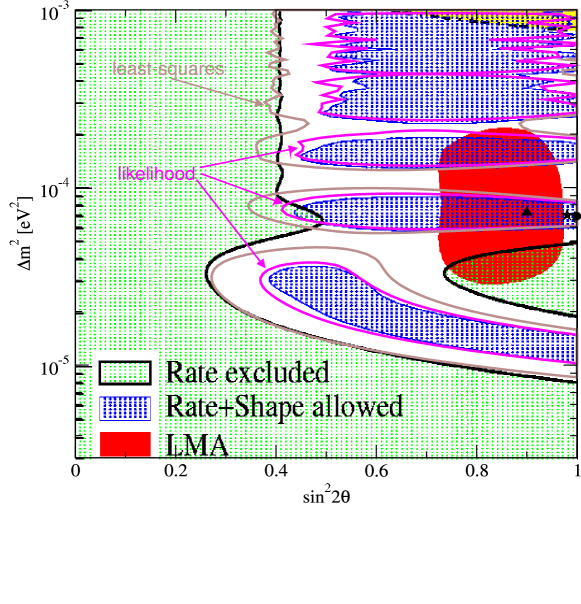
Figure 1: Comparison of the 95% CL regions obtained from the likelihood and the least-squares methods (lines) with the ones published by the KamLAND collaboration kamlandPRL (regions labeled as “Rate+Shape allowed”). The best fit points are marked by a star, triangle, dot for the likelihood, least-squares, KamLAND analyses, respectively.

2.2 Least-squares analysis of KamLAND data

The least-squares analyses performed by many authors Maltoni:2002aw , Fogli:2002au , Bahcall:2002ij , Bandyopadhyay:2002en , deHolanda:2002iv , Creminelli:2001ij , Aliani:2002na , Barger:2002at , Nunokawa:2002mq , Balantekin:2003dc are based on the KamLAND data binned into 13 energy intervals, $N^{i}_{\mathrm{obs}},\,i=1,\ldots,13$, as given in Fig. 5 of Ref. kamlandPRL . Since the number of events in the individual bins is rather small (in some bins even zero) the use of a least-squares statistic based on the Poisson distribution is appropriate pdg :

$$X^{2}(\sin^{2}2\theta,\Delta m^{2})=2\sum_{i}\left\{\alpha N^{i}_{\mathrm{pred}}-N^{i}_{\mathrm{obs}}+N^{i}_{\mathrm{obs}}\ln\frac{N^{i}_{\mathrm{obs}}}{\alpha N^{i}_{\mathrm{pred}}}\right\}+\left(\frac{1-\alpha}{\sigma_{\mathrm{syst}}}\right)^{2}\,,$$ (10)

where the term containing the logarithm is absent in bins with no events. The predicted number of events $N^{i}_{\mathrm{pred}}(\sin^{2}2\theta,\Delta m^{2})$ in bin $i$ is obtained by integrating the spectrum Eq. (2.1) over the prompt energy interval corresponding to that bin. Eq. (10) has to be minimised with respect to $\alpha$ in order to take into account the overall uncertainty of the theoretical predictions $\sigma_{\mathrm{syst}}=6.42\%$ kamlandPRL . Although the “least-squares” character of the statistic $X^{2}$ in Eq. (10) is not explicitly visible due to the use of the Poisson distribution it is denoted here by this term to stress the analogy to the commonly used “$\chi^{2}$-function”. A comparison of KamLAND analyses using Gaussian and Poisson least-squares functions can be found in Ref. Maltoni:2002aw .

The best fit parameters obtained by minimising Eq. (10) are $\Delta m^{2}=7.24\times 10^{-5}$ eV² and $\sin^{2}2\theta=0.90$. Assuming that

$$\Delta X^{2}(\sin^{2}2\theta,\Delta m^{2})=X^{2}(\sin^{2}2\theta,\Delta m^{2})-X^{2}_{\mathrm{min}}$$ (11)

follows a $\chi^{2}$-distribution with 2 degrees of freedom approximate confidence regions are obtained by considering contours of constant $\Delta X^{2}$ according to the $\chi^{2}$-cut method in Eq. (1). From Fig. 1 we find that the 95% confidence regions obtained by this method are significantly larger than the ones from the likelihood analysis and the regions published by the KamLAND collaboration. This fact was already noted in Ref. Fogli:2002au . I conclude that the loss of information implied by the binning of the data is not negligible, and the likelihood analysis provides a more powerful method to extract information from the current KamLAND data sample. Note, however, that in future the differences between the two methods are expected to decrease, since if more data is available a smaller bin size can be chosen, and in the limit of zero bin width the least-squares method converges to the un-binned likelihood method.

3 Confidence regions with correct coverage

Since the number of events in the currently available KamLAND data sample is rather small the question arises, whether the standard procedures to calculate confidence regions as described in Sec. 2 are reliable. Especially the assumption concerning the distribution of $\Delta X^{2}$ might be not justified. Moreover, the parameters of interest, $\Delta m^{2}$ and $\sin^{2}2\theta$, enter the problem in a highly non-linear way, which leads to multiple local maxima of the likelihood function (or local minima of the $X^{2}$-statistic). In such a case the actual confidence level of the parameter regions obtained from Eq. (1) may differ significantly from the canonical value $\beta$. To check the robustness of the results I have calculated frequentist confidence regions, where the correct coverage is guaranteed by construction. To this aim I follow the prescription given by Feldman and Cousins in Ref. FC .

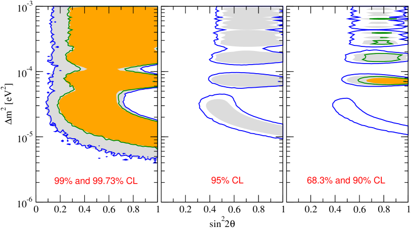
Figure 2: Comparison of confidence regions with correct coverage (lines) with the regions obtained from the $\chi^{2}$-cut approximation (shaded regions) for the likelihood method.

For both approaches discussed above – likelihood as well as least-squares methods – many synthetic data sets are simulated for fixed oscillation parameters. In the case of the likelihood method first the number of events in the synthetic data sample $N_{\mathrm{sim}}(\sin^{2}2\theta,\Delta m^{2})$ is generated from a Gaussian distribution with mean $N_{\mathrm{pred}}(\sin^{2}2\theta,\Delta m^{2})$ and standard deviation $\sigma_{\mathrm{rate}}$ given in Eq. (8). Then the prompt energies of the $N_{\mathrm{sim}}$ events is thrown according to the distribution Eq. (4). To test the least-squares method a value $\alpha_{\mathrm{sim}}$ for the parameter $\alpha$ describing the normalisation uncertainty in Eq. (10) is generated from a Gaussian distribution with mean 1 and standard deviation $\sigma_{\mathrm{syst}}$. Then the number of events in each bin $i$ is simulated from a Poisson distribution with the mean $\alpha_{\mathrm{sim}}N_{\mathrm{pred}}^{i}(\sin^{2}2\theta,\Delta m^{2})$.

Each “data set” generated this way is analysed as described in Sec. 2 in order to calculate $\Delta X^{2}(\sin^{2}2\theta,\Delta m^{2})$. For each point on a sufficiently dense grid in the $(\sin^{2}2\theta,\Delta m^{2})$ plane this has been done $10^{4}$ times for the likelihood method and $10^{5}$ times for the least-squares method to map out the actual distribution of $\Delta X^{2}$ in that point: $p_{\mathrm{sim}}(\Delta X^{2};\,\sin^{2}2\theta,\Delta m^{2})$. Then, in analogy to Eq. (1), the point $(\sin^{2}2\theta,\Delta m^{2})$ is included in the confidence region at $\beta$ CL if $\Delta X_{\mathrm{data}}^{2}(\sin^{2}2\theta,\Delta m^{2})$ obtained from the real data is smaller than the one of $100\beta\%$ of the simulated data sets in that point in the parameter space:

$$\Delta X_{\mathrm{data}}^{2}(\sin^{2}2\theta,\Delta m^{2})\leq X^{2}_{\beta}\,,\quad\mbox{where}\quad\int_{0}^{X^{2}_{\beta}}p_{\mathrm{sim}}(x;\,\sin^{2}2\theta,\Delta m^{2}){\rm d}x=\beta\,.$$ (12)

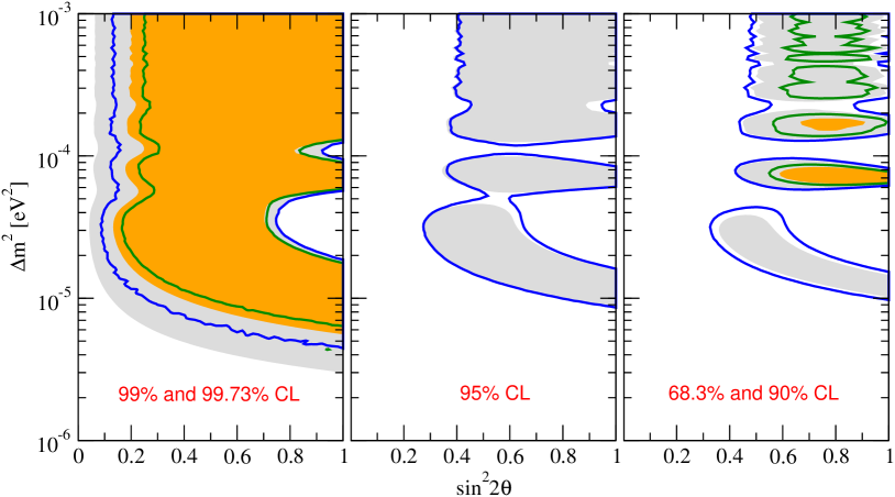
Figure 3: Comparison of confidence regions with correct coverage (lines) with the regions obtained from the $\chi^{2}$-cut approximation (shaded regions) for the least-squares method.

The results of these analyses are shown in Figs. 2 and 3 for the likelihood and the least-squares methods, respectively. The regions with correct coverage are compared to the ones obtained by the $\chi^{2}$-cut approximation. In both cases reasonable agreement of the exact and approximate confidence regions is found, although quantitative differences are visible. For the likelihood method the regions at 99.73% and 99% CL are in excellent agreement, whereas for lower confidence levels the $\chi^{2}$-cut approximation gives regions somewhat smaller than the exact ones. Especially the region $10^{-5}$ eV${}^{2}\lesssim\Delta m^{2}\lesssim 4\times 10^{-5}$ eV² does not appear at 90% CL for the $\chi^{2}$-cut approximation. In the case of the least-squares method the 95% CL regions are in excellent agreement. For higher confidence levels the $\chi^{2}$-cut approximation gives regions somewhat larger than the exact ones, whereas for lower confidence levels the allowed regions are a bit underestimated. E.g., the region $\Delta m^{2}\gtrsim 2\times 10^{-4}$ eV² does not appear at 68.3% CL for the $\chi^{2}$-cut approximation. In general the $\chi^{2}$-cut approximation works quite well in the vicinity of the best fit point around $\Delta m^{2}\approx 7\times 10^{-5}$ eV².

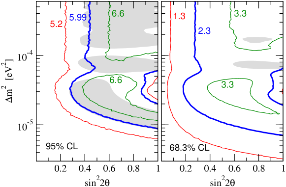
Figure 4: Contours of constant $X^{2}_{\beta}$ as defined in Eq. (12) for the least-squares method for $\beta=0.95$ (left panel) and $\beta=0.683$ (right panel). The thick lines correspond to the values which would result from a $\chi^{2}$-distribution with 2 degrees of freedom. The shaded regions are the approximate allowed regions from the $\chi^{2}$-cut method.

A better understanding of these results can be obtained by considering how $X^{2}_{\beta}$ defined in Eq. (12) varies as a function of the oscillation parameters. Note that this quantity does not depend on the actually observed data; it characterises the properties of the statistical method applied to the specific experimental setup. For definiteness I consider the least-squares method, for which contours of constant $X^{2}_{\beta}$ are shown in Fig. 4 for $68.3\%$ and $95\%$ CL. In the left panel of that figure one can see that the contour for $X^{2}_{0.95}=5.99$, which corresponds to the $\chi^{2}$-distribution for 95% CL, happens to be rather close to the 95% CL region from the $\chi^{2}$-cut approximation. This explains the good agreement observed in the middle panel of Fig. 3. Furthermore, one finds from Fig. 4 that $X^{2}_{\beta}$ decreases for small values of $\sin^{2}2\theta$ and $\Delta m^{2}$. The reason for this behaviour can be understood as follows: If $\sin^{2}2\theta$ becomes $\lesssim 0.2$ and/or $\Delta m^{2}\lesssim 10^{-5}$ eV² the effect of oscillations gets very small, and the signal in KamLAND corresponds roughly to the no-oscillation case. Analysing data generated from parameters in that region leads to best fit points also in the no-oscillation region, with a rather similar $X^{2}$. Hence, the distribution of $\Delta X^{2}$ is more peaked at low values, which implies relatively small values of $X^{2}_{\beta}$. This explains the tendency of more constraining exact confidence regions for small values of $\sin^{2}2\theta$ and $\Delta m^{2}$. The physical reason for this behaviour is that even with the present KamLAND data sample no-disappearance can be very well distinguished from oscillations with $\sin^{2}2\theta\gtrsim 0.2$ and $\Delta m^{2}\gtrsim 10^{-5}$ eV². Moreover, in the region of small $\sin^{2}2\theta$ or $\Delta m^{2}$ the full 2-parameter dependence of the survival probability is lost, and the effective number of degrees of freedom is reduced, leading to smaller values of $X^{2}_{\beta}$. The reason why for the likelihood method the agreement is better for higher CL than for the least-squares method can be partially attributed to the fact that for the latter the approximate regions extend to smaller values of $\sin^{2}2\theta$, which implies smaller values of $X^{2}_{\beta}$ and larger disagreement with the $\chi^{2}$-approximation.

In contrast, for $\sin^{2}2\theta\gtrsim 0.4$ and $\Delta m^{2}\gtrsim 10^{-5}$ eV² the simulation yields relatively higher values of $X^{2}_{\beta}$. In that region oscillations are important. However, because of the rather small data sample the signature of given parameters can not be identified with sufficiently high significance. This implies that statistical fluctuations can lead easily to best fit points in a different local minimum. In other words, when data are generated by given parameters in that region, fluctuations can mimic a signal which is better fitted by quite different parameters. Hence, the best fit points are stronger affected by fluctuations, resulting into a broader distribution of $\Delta X^{2}$ and larger values of $X^{2}_{\beta}$. From Fig. 4 one observes that the approximate confidence regions at 68.3% CL are well inside the high $X^{2}_{\beta}$ regime. This explains the weaker constraints from exact allowed regions for low confidence levels in Fig. 3. Note, however, that in the region around $\Delta m^{2}\sim 7\times 10^{-5}$ eV², where KamLAND is most sensitive to oscillations, the $X^{2}_{\beta}$ values decrease again. This shows that in that region KamLAND can well identify the parameters, leading already to statistical properties close to the expected $\chi^{2}$-distribution. Therefore, around the best fit point exact and approximate confidence regions are in good agreement.

The main conclusion to be drawn from Figs. 2 and 3 is that already using the current 54 events from KamLAND the approximate $\chi^{2}$-cut method gives a rather reliable determination of allowed regions. The small quantitative differences to exact confidence regions can be understood by considering the impact of statistical fluctuations on the fit. One may expect that once more data will have been collected the differences will further decrease, because statistical fluctuations will be less important. Furthermore, if the true oscillation parameters happen to be close to the present best fit region around $\Delta m^{2}\sim 7\times 10^{-5}$ eV² and large $\sin^{2}2\theta$ a rather clear oscillation signal can be observed in KamLAND. In that case the impact of other local minima will become small and one may expect that $\Delta X^{2}$ will follow a distribution rather close to the $\chi^{2}$-distribution.

4 Have we already observed oscillations in KamLAND?

Because of the limited statistics of the current KamLAND data sample the data is consistent with an energy independent suppression of the reactor neutrino flux kamlandPRL . This is evident, since allowed regions appear for large $\Delta m^{2}$, corresponding to energy averaged oscillations. However, even this first data set indicates some spectral distortion which is consistent with neutrino oscillations. In this section the statistical significance for an oscillatory signal is quantified by using a so-called decoherence parameter. The survival probability for the electron anti-neutrinos is modified (in a rather arbitrary way) by multiplying the quantum mechanical interference term which leads to the oscillatory behaviour by a factor $(1-\zeta)$:

$$P=1-\frac{1}{2}\,\sin^{2}2\theta\left[1-(1-\zeta)\cos\frac{\Delta m^{2}L}{2E_{\nu}}\right]\,.$$ (13)

Restricting $\zeta$ to the interval $[0,1]$ one can describe in a model independent way a loss of quantum mechanical coherence due to some unspecified mechanism. $\zeta=0$ corresponds to standard quantum mechanics, whereas $\zeta=1$ describes complete decoherence, i.e., an energy and baseline independent suppression of the flux.

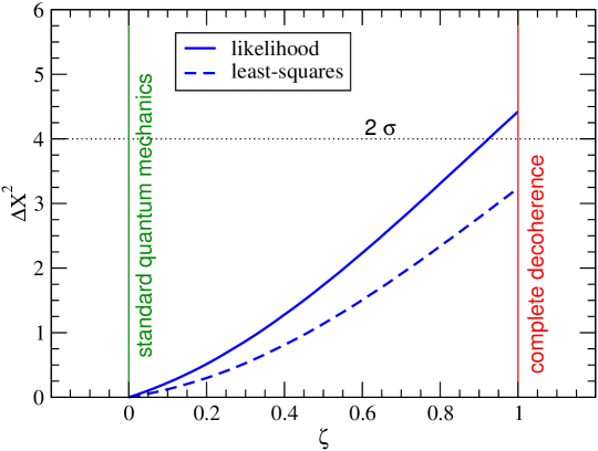
Figure 5: $\Delta X^{2}$ as a function of the decoherence parameter $\zeta$ for the likelihood and the least-squares method.

Now the data is analysed as a function of the three parameters $\Delta m^{2},\sin^{2}2\theta$ and $\zeta$. The $\Delta X^{2}$ marginalised with respect to $\Delta m^{2}$ and $\sin^{2}2\theta$ is shown in Fig. 5 for the likelihood and the least-squares method. A clear indication in favour of oscillations is observed. Complete decoherence is disfavoured with $\Delta X^{2}=4.4$ using the likelihood method and $\Delta X^{2}=3.2$ by the least-squares method. This confirms that the likelihood method is a more powerful tool to extract spectral information from the data, in agreement with the results of Sec. 2. Assuming that $\Delta X^{2}(\zeta)$ is distributed as a $\chi^{2}$ with 1 degree of freedom I conclude that the current KamLAND data provides a $\sim 2\sigma$ indication in favour of neutrino oscillations, implying quantum mechanical interference over distances of the order of 200 km.

Depending on the true values of the oscillation parameters one may expect that the statistical significance for oscillations in KamLAND will strongly improve by future data. A simple rescaling of the current data by a factor 5 leads to an exclusion of complete decoherence at $3.7\sigma$ if the true value of $\Delta m^{2}$ turns out to be $7\times 10^{-5}$ eV². On the other hand if $\Delta m^{2}=1.5\times 10^{-4}$ eV² decoherence can be excluded only at $2.6\sigma$, since for large $\Delta m^{2}$ the baselines in KamLAND are too long to be sensitive to the oscillations.

5 Conclusions

In this letter two different analysis methods for the first data from the KamLAND reactor neutrino experiment have been compared. I found that an event-by-event based likelihood method provides a more powerful tool to extract information on two-neutrino oscillation parameters than a least-squares method based on energy binned data. The likelihood method takes into account the precise energy information contained in each single event and avoids the information loss due to binning. Furthermore, exact frequentist confidence regions in the parameter space have been calculated by means of Monte Carlo simulation according to the Feldman-Cousins method FC . This method properly accounts for the non-linearity of the oscillation parameters $\sin^{2}2\theta$ and $\Delta m^{2}$, and statistical fluctuations in the data, which can be quite large due to the rather small number of events in the current data sample. I have found a reasonable agreement of the exact confidence regions with the ones obtained from the $\chi^{2}$-cut approximation, especially in the vicinity of the best point at $\Delta m^{2}\approx 7\times 10^{-5}$ eV². However, depending on the analysis method (likelihood or least-squares) quantitative differences are visible, especially for lower confidence levels and far from the best fit point. Finally, although the current data is consistent with an energy independent flux suppression, a $\sim 2\sigma$ indication in favour of oscillations can be stated using the likelihood method, which is especially sensitive to the spectral shape information. Put in other words, this implies a $\sim 2\sigma$ evidence for quantum mechanical interference over distances of the order of 200 km.

In summary, the results obtained in this work confirm that even for the limited statistics of the current KamLAND data sample the $\chi^{2}$-cut approximation to calculate confidence regions for the oscillation parameters gives rather reliable results. One expects that in future the agreement between approximate and exact confidence regions will improve due to increase in statistics. Moreover, the differences between likelihood and least-squares methods will become smaller.

Acknowledgements. I thank M. Maltoni and J.W.F. Valle for collaboration on the KamLAND analysis. Furthermore, I would like to thank M. Lindner, P. Huber and T. Lasserre for very useful discussions. This work is supported by the “Sonderforschungsbereich 375-95 für Astro-Teilchenphysik” der Deutschen Forschungsgemeinschaft.

References

- [1] K. Eguchi et al. [KamLAND Coll.], Phys. Rev. Lett. 90 (2003) 021802.
- [2] Q. R. Ahmad et al. [SNO Coll.], Phys. Rev. Lett. 87, 071301 (2001); ibid. 89 011301 (2002); S. Fukuda et al. [Super-Kamiokande Coll.], Phys. Lett. B 539, 179 (2002); B. T. Cleveland et al., Astrophys. J. 496, 505 (1998); J. N. Abdurashitov et al., J. Exp. Theor. Phys. 95, 181 (2002); W. Hampel et al. [GALLEX Coll.], Phys. Lett. B 447, 127 (1999); E. Bellotti [GNO Coll.], Nucl. Phys. B (Proc. Suppl.) 91, 44 (2001).
- [3] M. Maltoni, T. Schwetz and J. W. F. Valle, Phys. Rev. D 67 (2003) 093003 [arXiv:hep-ph/0212129].
- [4] G. L. Fogli et al., Phys. Rev. D 67 (2003) 073002 [arXiv:hep-ph/0212127].
- [5] J. N. Bahcall, M. C. Gonzalez-Garcia and C. Pena-Garay, JHEP 0302 (2003) 009 [arXiv:hep-ph/0212147].
- [6] A. Bandyopadhyay et al., Phys. Lett. B 559 (2003) 121 [arXiv:hep-ph/0212146].
- [7] P. C. de Holanda and A. Y. Smirnov, JCAP 0302 (2003) 001 [arXiv:hep-ph/0212270].
- [8] P. Creminelli, G. Signorelli and A. Strumia, arXiv:hep-ph/0102234 v4.
- [9] P. Aliani, V. Antonelli, M. Picariello and E. Torrente-Lujan, arXiv:hep-ph/0212212.
- [10] V. Barger and D. Marfatia, Phys. Lett. B 555 (2003) 144 [arXiv:hep-ph/0212126].
- [11] H. Nunokawa, W. J. Teves and R. Zukanovich Funchal, Phys. Lett. B 562 (2003) 28 [arXiv:hep-ph/0212202].
- [12] A. B. Balantekin and H. Yuksel, J. Phys. G 29 (2003) 665 [arXiv:hep-ph/0301072].
- [13] S. Pakvasa and J. W. F. Valle, arXiv:hep-ph/0301061.
- [14] G.J. Feldman and R.D. Cousins, Phys. Rev. D 57 (1998) 3873 [arXiv:physics/9711021].
- [15] G. Fiorentini, T. Lasserre, M. Lissia, B. Ricci and S. Schonert, Phys. Lett. B 558 (2003) 15 [arXiv:hep-ph/0301042].
- [16] A. Ianni, arXiv:hep-ph/0302230.
- [17] H. Cramér, Mathematical Methods of Statistics, Princeton Univ. Press 1946; A.G. Frodesen, O. Skjeggestad and H. Tofte, Probability and Statistics in Particle Physics, Universitatsforlaget, Bergen 1979.
- [18] K. Hagiwara et al., [Particle data goup] Phys. Rev. D66, 010001-1 (2002).
- [19] P. Vogel and J. F. Beacom, Phys. Rev. D 60, 053003 (1999) [arXiv:hep-ph/9903554].
- [20] P. Vogel and J. Engel, Phys. Rev. D 39, 3378 (1989).
- [21] J. Busenitz et al., 1999, Proposal for US Participation in KamLAND; The KamLAND proposal, Stanford-HEP-98-03.
- [22] J. R. Ellis, J. S. Hagelin, D. V. Nanopoulos and M. Srednicki, Nucl. Phys. B 241 (1984) 381.
- [23] E. Lisi, A. Marrone and D. Montanino, Phys. Rev. Lett. 85 (2000) 1166 [arXiv:hep-ph/0002053]; G. L. Fogli, E. Lisi, A. Marrone and D. Montanino, Phys. Rev. D 67 (2003) 093006 [arXiv:hep-ph/0303064].
- [24] R. A. Bertlmann and W. Grimus, Phys. Lett. B 392 (1997) 426 [arXiv:hep-ph/9610301]; R. A. Bertlmann, W. Grimus and B. C. Hiesmayr, Phys. Rev. D 60 (1999) 114032 [arXiv:hep-ph/9902427].