Abstract

We study nuclear shadowing for transverse and longitudinal photons. The coherence length, which controls the onset of nuclear shadowing at small Bjorken-$x$, $x_{Bj}$, is longer for longitudinal than for transverse photons. The light-cone Green function technique properly treats the finite coherence length in all multiple scattering terms. This is especially important in the region $x_{Bj}>0.01$, where most of the data exist. NMC data on shadowing in deep inelastic scattering are well reproduced in this approach. We also incorporate nonperturbative effects, in order to extrapolate this approach to small photon virtualities $Q^{2}$, where perturbative QCD cannot be applied. This way, we achieve a description of shadowing that is based only on quark and gluon degrees of freedom, even at low $Q^{2}$.

Invited talk given at NAPP03 conference, Dubrovnik, Croatia, May 26 – 31, 2003.

1 Introduction

The use of nuclei instead of protons in high energy scattering experiments, such as deep inelastic scattering (DIS), provides unique possibilities to study the space-time development of strongly interacting systems. In experiments with proton targets the products of the scattering process can only be observed in a detector which is separated from the reaction point by a macroscopic distance. In contrast to this, the nuclear medium can serve as a detector located directly at the place where the microscopic interaction happens. As a consequence, with nuclei one can study coherence effects in QCD which are not accessible in DIS off protons nor in proton-proton scattering.

Figure 1: At low $x_{Bj}$ and in the target rest frame, the virtual photon $\gamma^{*}$ converts into a $q\bar{q}$-pair long before the target.

At high energies, nuclear scattering is governed by coherence effects which are most easily understood in the target rest frame. In the rest frame, DIS looks like pair creation from a virtual photon, see Fig. 1. Long before the target, the virtual photon splits into a $q\bar{q}$-pair. The lifetime $l_{c}$ of the fluctuation, which is also called coherence length, can be estimated with help of the uncertainty relation to be of order $\sim 1/m_{N}x_{Bj}$, where $x_{Bj}$ is Bjorken-x and $m_{N}\approx 1$ GeV is the nucleon mass. The coherence length can become much greater than the nuclear radius at low $x_{Bj}$. Multiple scattering within the lifetime of the $q\bar{q}$ fluctuation leads to the pronounced coherence effects observed in experiment.

The most prominent example for a coherent interaction of more than one nucleon is the phenomenon of nuclear shadowing, i.e. the suppression of the nuclear structure function $F_{2}^{A}$ with respect to the proton structure function $F_{2}^{p}$, $F_{2}^{A}(x_{Bj},Q^{2})/(AF_{2}^{p}(x_{Bj},Q^{2}))<1$, at low $x_{Bj}\mathrel{\hbox to0.0pt{\lower 4.0pt\hbox{\hskip 1.0pt$\sim$}\hss}\raise 1.0pt\hbox{$<$}}0.1$. Shadowing in low $x_{Bj}$ DIS and at high photon virtualities is experimentally well studied by NMC [1].

What is the mechanism behind this suppression? If the coherence length is very long, as indicated in Fig. 1, the $q\bar{q}$-dipole undergoes multiple scatterings inside the nucleus. The physics of shadowing in DIS is most easily understood in a representation, in which the pair has a definite transverse size $\rho$. As a result of color transparency [2, 3], small pairs interact with a small cross section, while large pairs interact with a large cross section. The term ”shadowing” can be taken literally in the target rest frame. Large pairs are absorbed by the nucleons at the surface which cast a shadow on the inner nucleons. The small pairs are not shadowed. They have equal chances to interact with any of the nucleons in the nucleus. From these simple arguments, one can already understand the two necessary conditions for shadowing. First, the hadronic fluctuation of the virtual photon has to interact with a large cross section and second, the coherence length has to be long enough to allow for multiple scattering.

2 Shadowing and diffraction in DIS

Like shadowing in hadron-nucleus collisions, shadowing in DIS is also intimately related to diffraction [4]. The close connection between shadowing and diffraction becomes most transparent in the formula derived by Karmanov and Kondratyuk [5]. In the double scattering approximation, the shadowing correction can be related to the diffraction dissociation spectrum, integrated over the mass,

$${\sigma^{\gamma^{*}A}}\approx A\sigma^{\gamma^{*}p}-{4\pi}\,\int dM^{2}_{X}\,\left.\frac{d\sigma(\gamma^{*}N\to XN)}{dM^{2}_{X}\,dt}\right|_{t\to 0}\times\int d^{2}bF_{A}^{2}(l_{c},b).$$ (1)

Here

$$F_{A}^{2}(l_{c},b)=\left|\int_{-\infty}^{\infty}dz\rho_{A}(b,z){\rm e}^{{\rm i}z/l_{c}}\right|^{2}$$ (2)

is the formfactor of the nucleus, which depends on the coherence length

$$l_{c}=\frac{2\nu}{Q^{2}+M_{X}^{2}},$$ (3)

$\nu$ is the energy of the $\gamma^{*}$ in the target rest frame and $M_{X}$ is the mass of the diffractively excited state. The coherence length can be estimated from the uncertainty relation and is the lifetime of the diffractively excited state. If $l_{c}\to 0$, the shadowing correction in Eq. (1) vanishes and one is left with the single scattering term $A\sigma^{\gamma^{*}p}$.

2.1 The dipole approach

Note that Eq. (1) is valid only in double scattering approximation. For heavy nuclei, however, higher order scattering terms will become important. These can be calculated, if one knows the eigenstates of the interaction. Fortunately, the eigenstates of the $T$ matrix (restricted to diffractive processes) were identified a long time ago in QCD [2, 6] as partonic configurations with fixed transverse separations in impact parameter space. For DIS, the lowest eigenstate is the $q\bar{q}$ Fock component of the photon. The total $\gamma^{*}$-proton cross section is easily calculated, if one knows the cross section $\sigma_{q\bar{q}}(\rho)$ for scattering a $q\bar{q}$-dipole of transverse size $\rho$ off a proton,

$$\sigma^{\gamma^{*}p}=\sum_{T,L}\int d\alpha d^{2}\rho\left|\Psi^{T,L}_{q\bar{q}}(\alpha,\rho)\right|^{2}\sigma_{q\bar{q}}(\rho).$$ (4)

Here, $\alpha$ is the longitudinal momentum fraction carried by the quark in Fig. 1. The light-cone wavefunctions $\Psi^{T,L}_{q\bar{q}}(\alpha,\rho)$ describe the splitting of a transverse ($T$) and longitudinal ($L$) photon into a $q\bar{q}$-pair. For small $\rho$, the light-cone wavefunctions can be calculated in perturbation theory (see e.g. [7] for explicit expressions), but at large $\rho$ non-perturbative effects become important. In Ref. [8], these effects have been modeled by introducing a harmonic oscillator potential between the quark and the antiquark, which leads to a modification of the light-cone wavefunctions. The strength of this potential has been determined from data for photoabsorption on protons. This justifies the application of the dipole formulation at low $Q^{2}$ and makes this approach an alternative to the vector dominance model (see e.g. Ref. [9]). At large $Q^{2}$, of course, the modified light-cone wavefunctions reduce to the perturbative ones.

The dipole cross section is governed by nonperturbative effects and cannot be calculated from first principles. We use the phenomenological parameterization that is fitted to HERA data on the proton structure function. Note that higher Fock-states of the photon, containing gluons, lead to an energy dependence of $\sigma_{q\bar{q}}$, which we do not write out explicitly.

The diffractive cross section can also be expressed in terms of $\sigma_{q\bar{q}}$. Since the cross section for diffraction is proportional to the square of the $T$-matrix element, $|\langle\gamma^{*}|T|X\rangle|^{2}$, the dipole cross section also enters squared,

$$\int dM^{2}_{X}\,\left.\frac{d\sigma(\gamma^{*}N\to XN)}{dM^{2}_{X}\,dt}\right|_{t\to 0}=\frac{\langle\sigma^{2}_{q\bar{q}}(\rho)\rangle}{16\pi},$$ (5)

where the brackets $\langle\dots\rangle$ indicate averaging over the light-cone wavefunctions like in Eq. (4). We point out that in order to reproduce the correct behavior of the diffractive cross section at large $M_{X}$, one has to include at least the $q\bar{q}G$ Fock-state of the $\gamma^{*}$. This correction is, however, of minor importance in the region where shadowing data are available.

2.2 The Green function technique

If one attempts to calculate shadowing from Eq. (1) with help of Eq. (5), one faces the problem that the nuclear form factor, Eq. (2), depends on the mass $M_{X}$ of the diffractively produced state, which is undefined in impact parameter representation. Only in the limit $l_{c}\gg R_{A}$, where $R_{A}$ is the nuclear radius, it is possible to resum the entire multiple scattering series in an eikonal-formula

$$\sigma^{\gamma^{*}A}=\left<2\int d^{2}b\left(1-\exp\left(-\frac{\sigma_{q\bar{q}}(\rho)}{2}T(b)\right)\right)\right>.$$ (6)

The nuclear thickness function $T(b)=\int_{-\infty}^{\infty}dz\,\rho_{A}(b,z)$ is the integral of nuclear density over longitudinal coordinate $z$ and depends on the impact parameter $b$. The condition $l_{c}\gg R_{A}$ makes sure that the $\rho$ does not vary during propagation through the nucleus (Lorentz time dilation) and one can apply the eikonal approximation.

The condition $l_{c}\gg R_{A}$ is however not fulfilled in experiment. For the case $l_{c}\sim R_{A}$, one has to take the variation of $\rho$ during propagation of the $q\bar{q}$ fluctuation through the nucleus into account, see Fig. 2. A widely used recipe is to replace $M_{X}^{2}\to Q^{2}$, so that $l_{c}\to 1/(2m_{N}x_{Bj})$ and one can apply the double scattering approximation. This recipe was, however, disfavored by our investigation [10]. Moreover, there is no simple recipe to include a finite $l_{c}$ into higher order scattering terms.

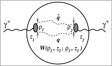
Figure 2: Propagation of a $q\bar{q}$-pair through a nucleus. Shown is the case of a finite coherence length, where the transverse motion is described by the Green function $W\left(\vec{\rho}_{2},z_{2}|\vec{\rho}_{1},z_{1}\right)$.

In Ref. [10] (see also Ref. [11]) a Green function technique was developed that provides the correct quantum-mechanical treatment of a finite coherence length in all multiple scattering terms. Like in Eq. (1) the total cross section is represented in the form

$$\sigma^{\gamma^{*}A}=A\sigma^{\gamma^{*}p}-\Delta\sigma,$$ (7)

where $\Delta\sigma$ is the shadowing correction,

$$\Delta\sigma = \frac{1}{2}{\rm Re}\sum_{T,L}\int d^{2}b\int\limits_{-\infty}^{\infty}dz_{1}\rho_{A}(b,z_{1})\int\limits_{z_{1}}^{\infty}dz_{2}\rho_{A}(b,z_{2})$$

$$\times \int_{0}^{1}d\alpha\int d^{2}\rho_{2}\left[\Psi_{q\bar{q}}^{T,L}(\vec{\rho}_{2},\alpha)\right]^{*}\sigma_{q\bar{q}}(\rho_{2})A(\vec{\rho}_{2},z_{1},z_{2},\alpha),$$

with

$$A(\vec{\rho}_{2},z_{1},z_{2},\alpha)=\int\,d^{2}\rho_{1}\,W(\vec{\rho}_{2},z_{2}|\vec{\rho}_{1},z_{1})\,{\rm e}^{-{\rm i}q_{L}^{min}(z_{2}-z_{1})}\,\sigma_{q\bar{q}}(\rho_{1})\,\Psi^{T,L}_{q\bar{q}}(\vec{\rho}_{1},\alpha).$$ (8)

Here,

$$q_{L}^{min}=\frac{1}{l_{c}^{max}}=\frac{Q^{2}\alpha(1-\alpha)+m_{f}^{2}}{2\nu\alpha(1-\alpha)}$$ (9)

is the minimal longitudinal momentum transfer when the photon splits into the $q\bar{q}$ dipole ($m_{f}$ is the quark mass).

The shadowing term in Eq. (7) is illustrated in Fig. 2. At the point $z_{1}$ the photon diffractively produces the $q\bar{q}$ pair ($\gamma^{*}N\to q\bar{q}N$) with a transverse separation $\vec{\rho}_{1}$. The pair propagates through the nucleus along arbitrarily curved trajectories, which are summed over, and arrives at the point $z_{2}$ with a separation $\vec{\rho}_{2}$. The initial and the final separations are controlled by the light-cone wavefunctions $\Psi^{T,L}_{q\bar{q}}(\vec{\rho},\alpha)$. While passing the nucleus the $q\bar{q}$ pair interacts with bound nucleons via the cross section $\sigma_{q\bar{q}}(\rho)$ which depends on the local separation $\vec{\rho}$. The Green function $W(\vec{\rho}_{2},z_{2}|\vec{\rho}_{1},z_{1})$ describes the propagation of the pair from $z_{1}$ to $z_{2}$, see Eq. (8), including all multiple rescatterings and a finite coherence length. Note the diffraction dissociation ($DD$) amplitude,

$$f_{DD}(\gamma^{*}\to q\bar{q})={\rm i}\Psi^{T,L}_{q\bar{q}}(\vec{\rho}_{1},\alpha)\sigma_{q\bar{q}}(\rho_{1}),$$ (10)

in Eq. (8). At the position $z_{2}$, the result of the propagation is again projected onto the diffraction dissociation amplitude. The Green function includes that part of the phase shift between the initial and the final photons which is due to transverse motion of the quarks, while the longitudinal motion is included in Eq. (8) through the exponential.

Figure 3: The $x_{Bj}$ dependence of shadowing in DIS for the structure function of tin relative to carbon. The data are from NMC [1]. The full curves are calculated in the Green-function approach, including the nonperturbative interaction between the $q$ and the $\bar{q}$. The dashed curve does not include this interaction. The figure is from Ref. [13].

The Green function $W(\vec{\rho}_{2},z_{2};\vec{\rho}_{1},z_{1})$ in Eq. (8) satisfies the two dimensional Schrödinger equation,

$${{\rm i}\,\frac{{\partial}W(\vec{\rho}_{2},z_{2}|\vec{\rho}_{1},z_{1})}{{\partial}z_{2}}=}-\frac{\Delta(\rho_{2})}{2\nu\alpha(1-\alpha)}\,W(\vec{\rho}_{2},z_{2}|\vec{\rho}_{1},z_{1})-{{\rm i}\over 2}\,\sigma(\rho_{2})\,\rho_{A}(b,z_{2})\,W(\vec{\rho}_{2},z_{2}|\vec{\rho}_{1},z_{1})$$ (11)

with the boundary condition $W(\vec{\rho}_{2},z_{1}|\vec{\rho}_{1},z_{1})=\delta^{(2)}(\vec{\rho}_{2}-\vec{\rho}_{1})$. The Laplacian $\Delta(\rho_{2})$ acts on the coordinate $\vec{\rho}_{2}$. The kinetic term $\Delta/[2\nu\alpha(1-\alpha)]$ in this Schrödinger equation takes care of the varying effective mass of the $q\bar{q}$ pair and provides the proper phase shift. The role of time is played by the longitudinal coordinate $z_{2}$. The imaginary part of the optical potential describes the rescattering. This equation has recently been solved numerically by Nemchik [12].

The Green function method contains the Karmanov-Kondratyuk formula Eq. (1) and the eikonal approximation Eq. (6) as limiting cases. In order to obtain the eikonal approximation, one has to take the limit $\nu\to\infty$. In this case, the kinetic energy term in Eq. (11) can be neglected and with $q_{L}^{min}\to 0$ one arrives after a short calculation at Eq. (6). One can also recover the Karmanov-Kondratyuk formula, when one neglects the imaginary potential in Eq. (11). Then $W$ becomes the Green function of a free motion.

Calculations in the Green function approach are compared to NMC data in Fig. 3. Note that the leading twist contribution to shadowing is due to large dipole sizes, where nonperturbative effects, such as an interaction between the $q$ and the $\bar{q}$, might become important (see above). Therefore, the solid curve is calculated with the modified light-cone wavefunctions of Ref. [8]. The dashed curve is calculated with the conventional, perturbative light-cone wavefunctions, but including a constituent quark mass. Both curves are in reasonable agreement with the data. We stress that the Green function technique also takes into account some higher twist corrections to shadowing. This is essential for a successful description of the NMC data. In fact, it has been demonstrated in Ref. [14] that the leading twist approximation only poorly reproduces NMC data for shadowing in calcium.

Note that for the data shown in Fig. 3, the coherence length is of order of the nuclear radius or smaller. Indeed, shadowing vanishes around $x_{Bj}\approx 0.1$, because the coherence length becomes smaller than the mean internucleon spacing. Therefore, the eikonal approximation, Eq. (6), cannot be applied for the kinematics of NMC and a correct treatment of the coherence length becomes crucial. We emphasize that the calculation in Fig. 3 does not contain any free parameters. Following the spirit of Glauber theory, all free parameters are adjusted to DIS off protons.

2.3 Higher Fock states and the leading twist gluon shadowing

The shadowing for quarks discussed in the previous subsection is dominated by the transverse photon polarization. Longitudinal photons, on the other hand, can serve to measure the gluon density because they effectively couple to color-octet-octet dipoles. This can be understood in the following way: the light-cone wave function for the transition $\gamma^{*}_{L}\to q\bar{q}$ does not allow for large, aligned jet configurations as is the case for transversely polarized photons. Thus, all $q\bar{q}$ dipoles from longitudinal photons have size $1/Q^{2}$ and the double-scattering term vanishes $\propto 1/Q^{4}$. The leading-twist contribution for the shadowing of longitudinal photons arises from rescattering of the $|q\bar{q}G\rangle$ Fock state of the photon. Here again, the distance between the $q$ and the $\bar{q}$ is of order $1/Q^{2}$, but the gluon can propagate relatively far from the $q\bar{q}$-pair. In addition, after radiation of the gluon, the pair is in an octet state. Therefore, the entire $|q\bar{q}G\rangle$-system appears as a $GG$-dipole, and the shadowing correction to the longitudinal cross section can be identified with gluon shadowing.

A critical issue for determining the magnitude of gluon shadowing is the distance the gluon can propagate from the $q\bar{q}$-pair in impact parameter space, i.e. knowing how large the $GG$ dipole can become. This value has been extracted from single diffraction data in hadronic collisions in Ref. [8] because these data allow the diffractive gluon radiation (the triple-Pomeron contribution in Regge phenomenology) to be unambiguously singled out. The diffraction cross section ($\propto\rho^{4}$) is even more sensitive to the dipole size than the total cross section ($\propto\rho^{2}$) and is therefore a sensitive probe of the mean transverse separation. It was found in Ref. [8] that the mean dipole size must be of the order of $r_{0}=0.3\,\,\mbox{fm}$, considerably smaller than a light hadron. A rather small gluon cloud of this size surrounding the valence quarks is the only way that is known to resolve the long-standing problem of the small size of the triple-Pomeron coupling. The smallness of the $GG$ dipole is incorporated into the LC approach by a nonperturbative interaction between the gluons.

Figure 4: The $x$- and $Q^{2}$-dependence of gluon shadowing for carbon, copper and gold. The $x$-dependence is shown for $Q^{2}=20$ GeV², while the figure on the right is calculated for $x=10^{-4}$.

We calculate gluon shadowing as function of $x$ at fixed $Q^{2}$ and as a function of $Q^{2}$ at fixed $x$, integrated over the impact parameter $b$. The results are shown in Fig. 4. In the left-hand plot, one observes that gluon shadowing vanishes for $x>0.01$. This happens because the lifetime of the $|q\bar{q}G\rangle$-fluctuation becomes smaller than the mean internucleon distance of $\sim 2$ fm as $x$ exceeds $0.01$. Indeed, in Ref. [15] an average coherence length of slightly less than $2$ fm was found for the $|q\bar{q}G\rangle$-state at $x=0.01$ and large $Q^{2}\gg 1/r_{0}^{2}$. Note that gluon shadowing sets in at a smaller value of $x$ than quark shadowing because the mass of a $|q\bar{q}G\rangle$-state is larger than the mass of a $|q\bar{q}\rangle$-state. We also point out that gluon shadowing is weaker than quark shadowing in the $x$-range plotted, because the small size of the $GG$-dipole overcompensates the Casimir factor in the $GG$-proton cross section, $\sigma_{GG}=(9/4)\sigma_{q\bar{q}}$. Note however that at this time, almost nothing is known about gluon shadowing from experiment, and theoretical approaches differ vastly (see e.g. Ref. [16] for a comparison of different models). The plot on the right-hand side of Fig. 4 shows the $Q^{2}$-dependence of gluon shadowing and clearly demonstrates that gluon shadowing is a leading-twist effect, with $R_{G}$ only very slowly (logarithmically) approaching unity as $Q^{2}\to\infty$.

2.4 The mean coherence length

The importance of the coherence length $l_{c}$ was already mentioned above: this quantity controls the onset of quark and gluon shadowing at small $x_{Bj}$ and therefore governs shadowing in the kinematical region that is of interest for most experiments. The Green function technique is the only known way to include the quantum mechanically correct coherence length into all multiple scattering terms. However, since $l_{c}$ is not well defined in impact parameter space, it appears only implicitly in the Green function approach. It is therefore useful to introduce the concept of a mean coherence length, as it was done in Ref. [15].

A photon of virtuality $Q^{2}$ and energy $\nu$ can develop a hadronic fluctuation for a lifetime,

$$l_{c}=\frac{2\,\nu}{Q^{2}+M_{q\bar{q}}^{2}}=\frac{P}{x_{Bj}\,m_{N}}\ ,$$ (12)

where $M_{q\bar{q}}$ is the effective mass of the fluctuation, and the factor $P^{-1}=(1+M_{q\bar{q}}^{2}/Q^{2})$. The usual approximation is to assume that $M_{q\bar{q}}^{2}\approx Q^{2}$ since $Q^{2}$ is the only large dimensional scale available. In this case $P=1/2$.

The effective mass of a non-interacting $q\bar{q}$-pair is well defined, $M_{q\bar{q}}^{2}=(m_{f}^{2}+p_{T}^{2})/\alpha(1-\alpha)$, where $p_{T}$ and $\alpha$ are the transverse momentum and fraction of the light-cone momentum of the photon carried by the quark, respectively. Therefore, $P$ has a simple form,

$$P(k_{T},\alpha)=\frac{Q^{2}\,\alpha\,(1-\alpha)}{p_{T}^{2}+\varepsilon^{2}}\ ,$$ (13)

where $\varepsilon^{2}=\alpha(1-\alpha)Q^{2}+m_{f}^{2}$.

To find the mean lifetime of those fluctuations that contribute to shadowing, one should define the averaging procedure as

$$\langle P\rangle=\frac{\Bigl{\langle}f(\gamma^{*}\to q\bar{q})\Bigl{|}P(p_{T},\alpha)\Bigr{|}f(\gamma^{*}\to q\bar{q})\Bigr{\rangle}}{\Bigl{\langle}f(\gamma^{*}\to q\bar{q})\Bigl{|}f(\gamma^{*}\to q\bar{q})\Bigr{\rangle}}\ ,$$ (14)

where $f(\gamma^{*}\to q\bar{q})$ is the amplitude of diffractive dissociation of the virtual photon on a nucleon, Eq. (10). That way, $P$ is weighted with the interaction cross section squared $\sigma^{2}_{q\bar{q}}(\rho)$ in the averaging procedure. Then, the mean value of the factor $P(\alpha,p_{T})$ reads for transverse and longitudinal photons,

$$\left\langle P^{T,L}\right\rangle=\frac{\int_{0}^{1}d\alpha\int\!d^{2}\rho_{1}d^{2}\rho_{2}\left[\Psi_{q\bar{q}}^{T,L}\left(\vec{\rho}_{2},\alpha\right)\right]^{*}\!\!\sigma_{q\bar{q}}\left(\rho_{2}\right)\widetilde{P}\left(\vec{\rho}_{2}-\vec{\rho}_{1},\alpha\right)\Psi_{q\bar{q}}^{T,L}\left(\vec{\rho}_{1},\alpha\right)\sigma_{q\bar{q}}\left(\rho_{1}\right)}{\int_{0}^{1}d\alpha\int d^{2}\rho\left|\Psi_{q\bar{q}}^{T,L}\left(\vec{\rho}_{,}\alpha\right)\sigma_{q\bar{q}}\left(\rho\right)\right|^{2}}$$ (15)

with

$$\widetilde{P}\left(\vec{\rho}_{2}-\vec{\rho}_{1},\alpha\right)=\int\frac{d^{2}p_{T}}{\left(2\pi\right)^{2}}\,{\exp\left(-{\rm i}\,\vec{p}_{T}\cdot\left(\vec{\rho}_{2}-\vec{\rho}_{1}\right)\right)}{P\left(\alpha,\rho\right)}.$$ (16)

Figure 5: The mean coherence length as function of $Q^{2}$. The curves are for $q\bar{q}$ fluctuations of transverse and longitudinal photons, and for $q\bar{q}G$ fluctuation, from the top to bottom, respectively. Dotted curves correspond to calculations with perturbative wavefunctions and an approximate dipole cross section $\propto\rho^{2}$. Dashed curves are the same, except the realistic parameterization of $\sigma_{q\bar{q}}(\rho)$ is employed (see Ref. [15] for details). The solid curves are calculated with the nonperturbative wavefunctions of Ref. [8]

Numerical results are shown in Fig. 5. Note that the nonperturbative interaction also modifies the invariant mass of the $q\bar{q}$ pair from Eq. (13). This was taken into account in Ref. [15]. One observes that the mean coherence length for longitudinal photons is approximately twice as long as for transverse photons. However, shadowing for the $q\bar{q}$ Fock component of a longitudinally polarized photon is higher twist (see above). The coherence length for the $q\bar{q}G$ Fock state of a longitudinal photon, which gives rise to leading twist gluon shadowing, is much shorter, resulting in a delayed onset of shadowing for gluons.

3 Summary

DIS at low $x_{Bj}$ is most naturally described in the color dipole formulation, because partonic configurations with fixed transverse separations in impact parameter space are eigenstates of the interaction. This salient feature allows one to calculate multiple scattering effects, such as nuclear shadowing, in a very easy way: at very high energies, one can simply eikonalize the dipole cross section. At realistic energies, however, corrections due to the finite lifetime $l_{c}$ of the $q\bar{q}$-pair become important. In Ref. [10], we succeeded in generalizing the Gauber-Gribov theory of nuclear shadowing by incorporating a finite $l_{c}$ into all multiple scattering terms, using a Green function technique. Since nuclear shadowing is dominated by large dipole sizes, a nonperturbative interaction in form of an harmonic oscillator potential between the quarks was introduced in Ref. [8]. This makes the dipole approach applicable at low $Q^{2}$. Note however that it is not necessary for this model to reproduce the vector meson masses or the coherence length of the vector dominance model [15].

The main nonperturbative input to all formulae, the dipole cross section, cannot be calculated from first principles. Instead we use a phenomenological parameterization for this quantity, which is determined from low $x_{Bj}$ DIS. In the spirit of Glauber theory, nuclear effects are then calculated without introducing any new parameters. This way a good description of NMC data on shadowing in DIS is achieved. We did not attempt to include antishadowing, since this effect probably is beyond the standard shadowing dynamics.

The parameterization of the dipole cross section effectively also includes higher Fock states (containing gluons) through its energy dependence. These higher Fock states are however excluded from nuclear effects, if one eikonalizes only the $q\bar{q}$ cross section. The most striking consequence is that gluon shadowing (i.e. shadowing for longitudinal photons) appears to be higher twist. This problem is overcome by calculating the rescattering of the $|q\bar{q}G\rangle$-Fock state of the virtual photon, which gives rise to the leading twist gluon shadowing. A detailed calculation is published in Refs. [8, 17]. We emphasize that gluon shadowing sets in at smaller $x_{Bj}$ than shadowing for quarks, because the larger mass of the $|q\bar{q}G\rangle$-Fock state leads to a shorter coherence length. This result is supported by a calculation of the mean coherence length [15]. Shadowing disappears, when the coherence length becomes shorter than the mean internucleon separation ($\sim 2\,\mbox{fm}$).

The main advantage of the dipole formulation and our motivation for pursuing this approach is the insight it provides into the dynamical origin of nuclear effects, which are calculated without free parameters. Note that a variety of other processes can be described in the dipole language, e.g. Drell-Yan (DY) dilepton production [18], gluon radiation [19] heavy quark [20] and quarkonium production [21]. A parameter free calculation of nuclear shadowing for DY for example is needed, if one aims at extracting the energy loss of a fast quark propagating through nuclear from DY data [22]. Furthermore, this approach can also be applied to calculate the Cronin effect at RHIC [23].

Finally, we point out that even though the mechanism of a hard reaction looks quite differently in the dipole formulation from what one is used to in the parton model, the equivalence between the dipole approach and the conventional parton model has been demonstrated (for single scattering) numerically [18] and analytically [24] for several processes.

Acknowledgments: I am grateful to the organizers of NAPP03 conference for inviting me to this stimulating meeting. This work was supported by the U.S. Department of Energy at Los Alamos National Laboratory under Contract No. W-7405-ENG-38.

References

- [1] M. Arneodo et al. [New Muon Collaboration], Nucl. Phys. B 481, 23 (1996).
- [2] A. B. Zamolodchikov, B. Z. Kopeliovich and L. I. Lapidus, JETP Lett. 33, 595 (1981) [Pisma Zh. Eksp. Teor. Fiz. 33, 612 (1981)];
- [3] G. Bertsch, S. J. Brodsky, A. S. Goldhaber and J. F. Gunion, Phys. Rev. Lett. 47, 297 (1981); S. J. Brodsky and A. H. Mueller, Phys. Lett. 206B, 685 (1988).
- [4] V. N. Gribov, Sov. Phys. JETP 29, 483 (1969) [Zh. Eksp. Teor. Fiz. 56, 892 (1969)].
- [5] V. Karmanov and L. Kondratyuk, JETP Lett. 18, 266 (1973).
- [6] H. I. Miettinen and J. Pumplin, Phys. Rev. D 18, 1696 (1978).
- [7] N. N. Nikolaev and B. G. Zakharov, Z. Phys. C 49, 607 (1991).
- [8] B. Z. Kopeliovich, A. Schäfer and A. V. Tarasov, Phys. Rev. D 62, 054022 (2000).
- [9] W. Melnitchouk and A. W. Thomas, Phys. Lett. B 317, 437 (1993).
- [10] B. Z. Kopeliovich, J. Raufeisen and A. V. Tarasov, Phys. Lett. B 440, 151 (1998); J. Raufeisen, A. V. Tarasov and O. O. Voskresenskaya, Eur. Phys. J. A 5, 173 (1999).
- [11] U. A. Wiedemann, Nucl. Phys. B 582, 409 (2000); B. G. Zakharov, Phys. Atom. Nucl. 61, 838 (1998) [Yad. Fiz. 61, 924 (1998)].
- [12] J. Nemchik, arXiv:hep-ph/0301043.
- [13] J. Raufeisen, Ph.D. thesis, Heidelberg, 2000, hep-ph/0009358.
- [14] L. Frankfurt, V. Guzey and M. Strikman, arXiv:hep-ph/0303022.
- [15] B. Z. Kopeliovich, J. Raufeisen and A. V. Tarasov, Phys. Rev. C 62, 035204 (2000)
- [16] N. Armesto, A. Capella, A. B. Kaidalov, J. Lopez-Albacete and C. A. Salgado, arXiv:hep-ph/0304119.
- [17] B. Z. Kopeliovich, J. Raufeisen, A. V. Tarasov and M. B. Johnson, Phys. Rev. C 67, 014903 (2003).
- [18] J. Raufeisen, J. C. Peng and G. C. Nayak, Phys. Rev. D 66, 034024 (2002).
- [19] B. Z. Kopeliovich, A. Schäfer and A. V. Tarasov, Phys. Rev. C 59, 1609 (1999), extended version in hep-ph/9808378.
- [20] N. N. Nikolaev, G. Piller and B. G. Zakharov, J. Exp. Theor. Phys. 81 (1995) 851 [Zh. Eksp. Teor. Fiz. 108 (1995) 1554]; Z. Phys. A 354, 99 (1996); C. B. Mariotto, M. B. Gay Ducati and M. V. Machado, Phys. Rev. D 66, 114013 (2002).
- [21] B. Z. Kopeliovich and J. Raufeisen, arXiv:hep-ph/0305094 (and references therein).
- [22] M. B. Johnson, et al. [FNAL E772 Collab.], Phys. Rev. Lett. 86, 4483 (2001); M. B. Johnson, et al., Phys. Rev. C 65, 025203 (2002)
- [23] B. Z. Kopeliovich, J. Nemchik, A. Schäfer and A. V. Tarasov, Phys. Rev. Lett. 88, 232303 (2002); B. Z. Kopeliovich, arXiv:nucl-th/0306044.
- [24] J. Raufeisen and J. C. Peng, Phys. Rev. D 67, 054008 (2003); M. A. Betemps, M. B. Ducati, M. V. Machado and J. Raufeisen, Phys. Rev. D 67, 114008 (2003).