CP violation in $B\to\Phi K_{S}$ in a model III 2HDM.

Chao-Shang Huang ^a and Shou-hua Zhu ^b

^a Institute of Theoretical Physics, Academia Sinica, Beijing 100080, China
^b Ottawa-Carleton Institute for Physics, Department of Physics, Carleton University, Ottawa, Canada K1S 5B6

The mixing induced time dependent CP asymmetry, direct CP asymmetry, and branching ratio in $B\to\Phi K_{S}$ in a model III 2HDM are calculated, in particular, neutral Higgs boson contributions are included. It is shown that satisfying all the relevant experimental constraints, for time dependent CP asymmetry $S_{\phi K}$ the model III can agree with the present data, $S_{\phi k}=-0.39\pm 0.41$, within the $1\sigma$ error, and the direct CP asymmetry which is zero in SM can be about $-8\%\sim-20\%$ in the reasonable regions of parameters.

1 Introduction

The recently reported measurements of time dependent CP asymmetries in $B\to\Phi K_{S}$ decays by BaBar [3]

$$\sin(2\beta(\Phi K_{S}))_{BaBar}=-0.19^{+0.52}_{-0.50}\pm 0.09$$ (1)

and Belle [4]

$$\sin(2\beta(\Phi K_{S}))_{Belle}=-0.73\pm 0.64\pm 0.18$$ (2)

result in the error weighted average

$$\sin(2\beta(\Phi K_{S}))_{ave}=-0.39\pm 0.41\;$$ (3)

with errors added in quadrature. The value in (2) corresponds to the coefficient of the sine term in the time dependent CP asymmetry [6], see Section IV. Belle also quotes a value for the direct CP asymmetry $A_{CP}=-C_{\Phi K}$, i.e.,  the cosine term, $C_{\Phi K}=-0.19\pm 0.30$ [4, 5]. Although there are at present large theoretical uncertainties in calculating strong phases, we still examine direct CP asymmetry in the paper in order to obtain qualitatively feeling for effects of new physics on CP violation.

In the SM the above asymmetry is related to that in $B\to J/\Psi K_{S}$ [7]-[10] by

$$\sin(2\beta(\Phi K))=\sin(2\beta(J/\Psi K)\!)\!+\!O(\lambda^{2}\!)$$ (4)

where $\lambda\simeq 0.2$ appears in Wolfenstein’s parameterization of the CKM matrix and $\sin(2\beta(J/\Psi K_{S,L}))_{world-ave}=+0.734\pm 0.054$. Therefore, (3) violates the SM at the 2.7 $\sigma$ deviation. The impact of these experimental results on the validity of CKM and SM is currently statistics limited. Future prospects at the $B$-factories are that the statistical error $\sigma_{\Phi K_{S}}(stat)$ can be expected to improve roughly by a factor of three with an increase of integrated luminosity from $0.1ab^{-1}$ to $1ab^{-1}$ [11] and it will take some time before we know the deviation with sufficient precision to draw final conclusions.

However, the possibility of a would-be measurement of $\sin(2\beta(\Phi K_{S}))=-0.39$ or a similar value which departs drastically from the SM expectation of (4) has attracted much interest to search for new physics, in particular, supersymmetry, two Higgs doublet model (2HDM), and model-independent way [12, 13]. In the paper we consider the decay $B\to\Phi K_{S}$ in a model III 2HDM. It is well-known that in the model III 2HDM the couplings involving Higgs bosons and fermions can have complex phases, which can induce CP violation effects, even in the simplest case in which all tree-level FCNC couplings are negligible. The effect of the color dipole operator on the phase from the decay amplitudes, $\Delta\Phi\equiv arg(\frac{\bar{A}}{A})$, in $b\rightarrow s\bar{s}s$ in the model III 2HDM has been studied in the second paper of ref. [12] by Hiller and the result is $\Delta\Phi\leq 0.2$ which is far from explaining the deviation. We would like to see if it is possible to explain the deviation in the model III 2HDM under all known experimental constraints by extending to include the neutral Higgs boson (NHB) contributions and calculate hadronic matrix elements to the $\alpha_{s}$ order. Some relevant Wilson coefficients at the leading order (LO) in the model III 2HDM have been given [14]. Because the hadronic matrix elements of relevant operators have been calculated to the $\alpha_{s}$ order [15], we can obtain the amplitude of the process to the $\alpha_{s}$ order if we know the relevant Wilson coefficients at the next to leading order (NLO). In the paper we calculate them at NLO in the model III 2HDM. Furthermore, as pointed in ref. [13] the NHB penguin induced operators contribute sizably to both the branching ratio (Br) and time dependent CP asymmetry $S_{\phi k}$ in supersymmetrical models. In the paper we calculate the Wilson coefficients of NHB penguin induced operators in the model III 2HDM. Our results show that in the model III 2HDM, the CP asymmetry $S_{\phi K}$ can agree with the present data, $S_{\phi k}=-0.39\pm 0.41$, within the $1\sigma$ error. Even if the $S_{\phi k}$ is measured to a level of $-0.4\pm 0.1$ in the future, the model III can still agree with the data at the $2\sigma$ level. And the direct CP asymmetry can reach about $-20\%$.

The paper is organized as follows. In section II we describe the model III 2HDM briefly. In section III we give the effective Hamiltonian responsible for $B\rightarrow\phi K_{s}$ in the model. In particular, we give the Wilson coefficients at NLO for the operators which exist in SM and at LO for the new operators which are induced by NHB penguins respectively. We present the decay amplitude and the CP asymmetry $S_{\phi K}$ in $B\rightarrow\phi K_{s}$ in Section IV. The Section V is devoted to numerical results. In Section VI we draw our conclusions and present some discussions.

2 Model III two-Higgs-doublet model (2HDM)

In model III 2HDM, both the doublets can couple to the up-type and down-type quarks, the details of the model can be found in Ref. [16]. The Yukawa Lagrangian relevant to our discussion in this paper is

$${\cal L}_{Y} = -\frac{g}{2M_{W}}(H^{0}\cos\alpha-h^{0}\sin\alpha)\biggr{(}\overline{U}M_{U}U+\overline{D}M_{D}D\biggr{)}$$ (5)

$$- \frac{H^{0}\sin\alpha+h^{0}\cos\alpha}{\sqrt{2}}\Biggr{[}\overline{U}\biggr{(}{\hat{\xi}}^{U}\hbox{$1\over 2$}(1+\gamma^{5})+{\hat{\xi}}^{U\dagger}\hbox{$1\over 2$}(1-\gamma^{5})\biggr{)}U$$

$$+\overline{D}\biggr{(}{\hat{\xi}}^{D}\hbox{$1\over 2$}(1+\gamma^{5})+{\hat{\xi}}^{D\dagger}\hbox{$1\over 2$}(1-\gamma^{5})\biggr{)}D\Biggr{]}$$

$$+ \frac{iA^{0}}{\sqrt{2}}\Biggr{[}\overline{U}\biggr{(}{\hat{\xi}}^{U}\hbox{$1\over 2$}(1+\gamma^{5})-{\hat{\xi}}^{U\dagger}\hbox{$1\over 2$}(1-\gamma^{5})\biggr{)}U-\overline{D}\biggr{(}{\hat{\xi}}^{D}\hbox{$1\over 2$}(1+\gamma^{5})-{\hat{\xi}}^{D\dagger}\hbox{$1\over 2$}(1-\gamma^{5})\biggr{)}D\Biggr{]}$$

$$-H^{+}\overline{U}\biggr{[}V_{\rm CKM}{\hat{\xi}}^{D}\hbox{$1\over 2$}(1+\gamma^{5})-{\hat{\xi}}^{U\dagger}V_{\rm CKM}\hbox{$1\over 2$}(1-\gamma^{5})\biggr{]}D$$

$$-H^{-}\overline{D}\biggr{[}{\hat{\xi}}^{D\dagger}V^{\dagger}_{\rm CKM}\hbox{$1\over 2$}(1-\gamma^{5})-V^{\dagger}_{\rm CKM}{\hat{\xi}}^{U}\hbox{$1\over 2$}(1+\gamma^{5})\biggr{]}U\;\;,$$

where $U$ represents the mass eigenstates of $u,c,t$ quarks and $D$ represents the mass eigenstates of $d,s,b$ quarks, $V_{\rm CKM}$ is the Cabibbo-Kobayashi-Maskawa matrix and the FCNC couplings are contained in the matrices $\hat{\xi}^{U,D}$. The Cheng-Sher ansatz for $\hat{\xi}^{U,D}$ is [16]

$$\hat{\xi}^{U,D}_{ij}=\lambda_{ij}\frac{g\sqrt{m_{i}m_{j}}}{\sqrt{2}M_{W}}$$ (6)

by which the quark-mass hierarchy ensures that the FCNC within the first two generations are naturally suppressed by the small quark masses, while a larger freedom is allowed for the FCNC involving the third generations. In the ansatz the residual degree of arbitrariness of the FC couplings is expressed through the $\lambda_{ij}$ parameters which are of order one and need to be constrained by the available experiments. In the paper we choose $\xi^{U,D}$ to be diagonal and set the u and d quark masses to be zero for the sake of simplicity so that besides Higgs boson masses only $\lambda_{ii}$, i=s, c, b, t, are the new parameters and will enter into the Wilson coefficients relevant to the process.

3 Effective Hamiltonian

The effective Hamiltonian for charmless B decays with $\Delta B=1$ is given by [13, 20]

$${\cal H}_{\rm eff} = \frac{G_{F}}{\sqrt{2}}\sum_{p=u,c}\!V_{pb}V^{*}_{ps}\bigg{(}C_{1}\,Q_{1}^{p}+C_{2}\,Q_{2}^{p}+\!\sum_{i=3,\dots,16}\![C_{i}\,Q_{i}+C_{i}^{\prime}\,Q_{i}^{\prime}]$$ (7)

$$+C_{7\gamma}\,Q_{7\gamma}+C_{8g}\,Q_{8g}+C_{7\gamma}^{\prime}\,Q_{7\gamma}^{\prime}+C_{8g}^{\prime}\,Q_{8g}^{\prime}\,\bigg{)}+\mbox{h.c.}\,$$

Here $Q_{i}$ are quark and gluon operators and are given by

$$Q_{1}^{p}=(\bar{s}_{\alpha}p_{\beta})_{V-A}(\bar{p}_{\beta}b_{\alpha})_{V-A},\;\;Q_{2}^{p}=(\bar{s}_{\alpha}p_{\alpha})_{V-A}(\bar{p}_{\beta}b_{\beta})_{V-A},$$

$$Q_{3(5)}=(\bar{s}_{\alpha}b_{\alpha})_{V-A}\sum_{q}(\bar{q}_{\beta}q_{\beta})_{V-(+)A},\;\;Q_{4(6)}=(\bar{s}_{\alpha}b_{\beta})_{V-A}\sum_{q}(\bar{q}_{\beta}q_{\alpha})_{V-(+)A},$$

$$Q_{7(9)}={3\over 2}(\bar{s}_{\alpha}b_{\alpha})_{V-A}\sum_{q}e_{q}(\bar{q}_{\beta}q_{\beta})_{V+(-)A},\;\;Q_{8(10)}={3\over 2}(\bar{s}_{\alpha}b_{\beta})_{V-A}\sum_{q}e_{q}(\bar{q}_{\beta}q_{\alpha})_{V+(-)A},$$

$$Q_{11(13)}=(\bar{s}\,b)_{S+P}\sum_{q}\,{m_{q}\lambda_{qq}^{*}(\lambda_{qq})\over m_{b}}(\bar{q}\,q)_{S-(+)P}\,,$$

$$Q_{12(14)}=(\bar{s}_{i}\,b_{j})_{S+P}\sum_{q}\,{m_{q}\lambda_{qq}^{*}(\lambda_{qq})\over m_{b}}(\bar{q}_{j}\,q_{i})_{S-(+)P}\,,$$

$$Q_{15}=\bar{s}\,\sigma^{\mu\nu}(1+\gamma_{5})\,b\sum_{q}\,{m_{q}\lambda_{qq}\over m_{b}}\bar{q}\,\sigma_{\mu\nu}(1+\gamma_{5})\,q\,,$$

$$Q_{16}=\bar{s}_{i}\,\sigma^{\mu\nu}(1+\gamma_{5})\,b_{j}\sum_{q}\,{m_{q}\lambda_{qq}\over m_{b}}\bar{q}_{j}\,\sigma_{\mu\nu}(1+\gamma_{5})\,q_{i}\,$$

$$Q_{7\gamma}={e\over 8\pi^{2}}m_{b}\bar{s}_{\alpha}\sigma^{\mu\nu}F_{\mu\nu}(1+\gamma_{5})b_{\beta},$$

$$Q_{8g}={g_{s}\over 8\pi^{2}}m_{b}\bar{s}_{\alpha}\sigma^{\mu\nu}G_{\mu\nu}^{a}{\lambda_{a}^{\alpha\beta}\over 2}(1+\gamma_{5})b_{\beta},$$ (8)

where $(V\pm A)(V\pm A)=\gamma^{\mu}(1\pm\gamma_{5})\gamma_{\mu}(1\pm\gamma_{5})$, $(\bar{q}_{1}q_{2})_{S\pm P}=\bar{q}_{1}(1\pm\gamma_{5})q_{2}$, $q=u,d,s,c,b$, $e_{q}$ is the electric charge number of $q$ quark, $\lambda_{a}$ is the color SU(3) Gell-Mann matrix, $\alpha$ and $\beta$ are color indices, and $F_{\mu\nu}$ [$G_{\mu\nu}$] are the photon [gluon] field strengths. The operators $Q_{i}^{\prime}$s are obtained from the unprimed operators $Q_{i}$s by exchanging $L\leftrightarrow R$. In eq.(7) operators $Q_{i}$, i11,…,16, are induced by neutral Higgs boson mediations [13].

The Wilson Coefficients $C_{i}$, i=1,…,10, have been calculated at LO [20, 14]. We calculate them at NLO in the NDR scheme and results are as follows.

$$C_{1}(M_{\rm W}) = \frac{11}{2}\;\frac{\alpha_{s}(M_{\rm W})}{4\pi}\,,$$ (9)

$$C_{2}(M_{\rm W}) = 1-\frac{11}{6}\;\frac{\alpha_{s}(M_{\rm W})}{4\pi}-\frac{35}{18}\;\frac{\alpha}{4\pi}\,,$$ (10)

$$C_{3}(M_{\rm W}) = -\frac{\alpha_{s}(M_{\rm W})}{24\pi}\left\{\widetilde{E}_{0}(x_{t})+E^{III}_{0}(y)\right\}+\frac{\alpha}{6\pi}\frac{1}{\sin^{2}\theta_{W}}\left[2B_{0}(x_{t})+C_{0}(x_{t})\right]\,,$$ (11)

$$C_{4}(M_{\rm W}) = \frac{\alpha_{s}(M_{\rm W})}{8\pi}\left\{\widetilde{E}_{0}(x_{t})+E^{III}_{0}(y)\right\}\,,$$ (12)

$$C_{5}(M_{\rm W}) = -\frac{\alpha_{s}(M_{\rm W})}{24\pi}\left\{\widetilde{E}_{0}(x_{t})+E^{III}_{0}(y)\right\}\,,$$ (13)

$$C_{6}(M_{\rm W}) = \frac{\alpha_{s}(M_{\rm W})}{8\pi}\left\{\widetilde{E}_{0}(x_{t})+E^{III}_{0}(y)\right\}\,,$$ (14)

$$C_{7}(M_{\rm W}) = \frac{\alpha}{6\pi}\left[4C_{0}(x_{t})+\widetilde{D}_{0}(x_{t})\right]\,,$$ (15)

$$C_{8}(M_{\rm W}) = 0\,,$$ (16)

$$C_{9}(M_{\rm W}) = \frac{\alpha}{6\pi}\left[4C_{0}(x_{t})+\widetilde{D}_{0}(x_{t})+\frac{1}{\sin^{2}\theta_{W}}(10B_{0}(x_{t})-4C_{0}(x_{t}))\right]\,,$$ (17)

$$C_{10}(M_{\rm W}) = 0\,,$$ (18)

$$C_{7\gamma}(M_{W}) = -\frac{A(x_{t})}{2}-\frac{A(y)}{6}|\lambda_{tt}|^{2}+B(y)\lambda_{tt}\lambda_{bb}e^{i\theta}\;,$$ (19)

$$C_{8G}(M_{W}) = -\frac{D(x_{t})}{2}-\frac{D(y)}{6}|\lambda_{tt}|^{2}+E(y)\lambda_{tt}\lambda_{bb}e^{i\theta}\;\;,$$ (20)

where $x_{t}=m_{t}^{2}/M_{W}^{2}$, and $y=m_{t}^{2}/M_{H^{\pm}}^{2}$. Here the Wilson coefficients $C_{7\gamma}$ and $C_{8g}$ at LO which are given in ref. [14] have also been written. The Wilson coefficients $C_{7\gamma}$ and $C_{8g}$ at NLO in SM have been given but they at NLO in model III 2HDM have not been calculated yet. Because we calculate the decay amplitude only to the $\alpha_{s}$ order it is enough to know them at LO. Here

$$A(x) = x\biggr{[}\frac{8x^{2}+5x-7}{12(x-1)^{3}}-\frac{(3x^{2}-2x)\ln x}{2(x-1)^{4}}\biggr{]}$$ (21)

$$B(y) = y\biggr{[}\frac{5y-3}{12(y-1)^{2}}-\frac{(3y-2)\ln y}{6(y-1)^{3}}\biggr{]}$$ (22)

$$D(x) = x\biggr{[}\frac{x^{2}-5x-2}{4(x-1)^{3}}+\frac{3x\ln x}{2(x-1)^{4}}\biggr{]}$$ (23)

$$E(y) = y\biggr{[}\frac{y-3}{4(y-1)^{2}}+\frac{\ln y}{2(y-1)^{3}}\biggr{]}\;\;$$ (24)

$$B_{0}(x_{t}) = \frac{1}{4}\left[\frac{x_{t}}{1-x_{t}}+\frac{x_{t}\ln x_{t}}{(x_{t}-1)^{2}}\right]\,,$$ (25)

$$C_{0}(x_{t}) = \frac{x_{t}}{8}\left[\frac{x_{t}-6}{x_{t}-1}+\frac{3x_{t}+2}{(x_{t}-1)^{2}}\ln x_{t}\right]\,,$$ (26)

$$D_{0}(x_{t}) = -\frac{4}{9}\ln x_{t}+\frac{-19x_{t}^{3}+25x_{t}^{2}}{36(x_{t}-1)^{3}}+\frac{x_{t}^{2}(5x_{t}^{2}-2x_{t}-6)}{18(x_{t}-1)^{4}}\ln x_{t}\,,$$ (27)

$$\widetilde{D}_{0}(x_{t}) = D_{0}(x_{t})-\frac{4}{9}\,.$$ (28)

and

$$E_{0}(x_{t}) = -\frac{2}{3}\ln x_{t}+\frac{x_{t}(18-11x_{t}-x_{t}^{2})}{12(1-x_{t})^{3}}+\frac{x_{t}^{2}(15-16x_{t}+4x_{t}^{2})}{6(1-x_{t})^{4}}\ln x_{t}\,,$$ (29)

$$\widetilde{E}_{0}(x_{t}) = E_{0}(x_{t})-\frac{2}{3}$$ (30)

$$E^{III}_{0}(y) = |\lambda_{tt}|^{2}\left\{\frac{16y-29y^{2}+7y^{3}}{36(1-y)^{3}}+\frac{2y-3y^{2}}{6(1-y)^{4}}\ln y\right\}.$$ (31)

The Wilson coefficients $C_{i}$, i=11,…,16, at the leading order can be obtained from $C_{Q1}$ and $C_{Q2}$ in Ref. [19]. The non-vanishing coefficients at $m_{W}$ are

$$C_{11}(M_{W}) = \frac{\alpha}{4\pi}\frac{m_{b}}{m_{\tau}\lambda_{\tau\tau}^{*}}\left(C_{Q1}-C_{Q2}\right)$$

$$C_{13}(M_{W}) = \frac{\alpha}{4\pi}\frac{m_{b}}{m_{\tau}\lambda_{\tau\tau}}\left(C_{Q1}+C_{Q2}\right).$$ (32)

We shall omitted the contributions of the primed operators in numerical calculations for they are suppressed by $m_{s}\over m_{b}$ in model III 2HDM.

For the process we are interested in this paper, the Wilson coefficients should run to the scale of $O(m_{b})$. $C_{1}-C_{10}$ are expanded to $O(\alpha_{s})$ and NLO RGEs should be used. However for the $C_{8g}$ and $C_{7\gamma}$, LO results should be sufficient. The details of the running of these Wilson coefficients can be found in Ref. [20]. The one loop anomalous dimension matrices of the NHB induced operators can be divided into two distangled groups [23]

O11−160O12-62superscript𝛾𝑅𝐿fragments fragmentsO11fragments160fragmentsO12-62\displaystyle\gamma^{(RL)}=\begin{tabular}[]{c|cccc}&$O_{11}$&$O_{12}$\\ \hline\cr$O_{11}$&$-16$&0\\ $O_{12}$&-6&$2$\end{tabular}

O11O12O11O12 (36)

and

$$\gamma^{(RR)}=\begin{tabular}[]{c|cccc}&$O_{13}$&$O_{14}$&$O_{15}$&$O_{16}$\\ \hline\cr$O_{13}$&$-16$&0&1/3&-1\\ $O_{14}$&-6&$2$&-1/2&-7/6\\ $O_{15}$&16&-48&$16/3$&0\\ $O_{16}$&-24&-56&6&$-38/3$\end{tabular}$$ (42)

For $Q_{i}^{\prime}$ operators we have

$$\gamma^{(LR)}=\gamma^{(RL)}~{}~{}~{}~{}~{}and~{}~{}~{}~{}~{}\gamma^{(LL)}=\gamma^{(RR)}\,.$$ (43)

Because at present no NLO Wilson coefficients $C_{i}^{(\prime)}$, i=11,…,16, are available we use the LO running of them in the paper.

4 The decay amplitude and CP asymmetry in $B_{d}^{0}\rightarrow\phi K_{S}$

We use the BBNS approach [18] to calculate the hadronic matrix elements of operators. In the approach the hadronic matrix element of a operator in the heavy quark limit can be written as

$$<\phi K|Q|B>=<\phi K|Q|B>_{f}[1+\sum r_{n}\alpha_{s}^{n}],$$ (44)

where $<\phi K|Q|B>_{f}$ indicates the naive factorization result. The second term in the square bracket indicates higher order $\alpha_{s}$ corrections to the matrix elements [18]. We calculate hadronic matrix elements to the $\alpha_{s}$ order in the paper. In order to see explicitly the effects of new operators in the model III 2HDM we divide the decay amplitude into two parts. One has the same form as that in SM, the other is new. That is, we can write the decay amplitude, to the $\alpha_{s}$ order, for $B\to\phi K$ in the heavy quark limit as [15, 21, 13]

$$A(B\to\phi K)={G_{F}\over\sqrt{2}}A<\phi|\bar{s}\gamma_{\mu}s|0><K|\bar{s}\gamma^{\mu}b|B>,$$

$$A=A^{o}+A^{n},$$ (45)

$$A^{o}=V_{ub}V^{*}_{us}[a_{3}^{u}+a_{4}^{u}+a_{5}^{u}-{1\over 2}(a_{7}^{u}+a_{9}^{u}+a_{10}^{u})+a_{10a}^{u}]$$

$$\;\;\;\;\;\;\;+V_{cb}V^{*}_{cs}[a_{3}^{c}+a_{4}^{c}+a_{5}^{c}-{1\over 2}(a_{7}^{c}+a_{9}^{c}+a_{10}^{c})+a_{10a}^{c})],$$ (46)

$$A^{n}=-V_{tb}V^{*}_{ts}\bigg{(}a_{4}^{neu}+{m_{s}\over m_{b}}[-{1\over 2}\lambda_{ss}^{*}(a_{12}+a_{12}^{\prime})+\lambda_{ss}\,{4m_{s}\over m_{b}}\,(a_{16}+a_{16}^{\prime})]\bigg{)}\,.$$ (47)

For the hadronic matrix elements of the vector current, we can write $<\phi|\bar{s}\gamma_{\mu}b|0>=m_{\phi}f_{\phi}\epsilon^{\phi}_{\mu}$ and $<K|\bar{s}\gamma^{\mu}b|B>=F_{1}^{B\to K}(q^{2})(p_{B}^{\mu}+p_{K}^{\mu})+(F^{B\to K}_{0}(q^{2})-F^{B\to K}_{1}(q^{2}))(m_{B}^{2}-m_{K}^{2})q^{\mu}/q^{2}$. Here, the coefficients $a_{i}^{u,c}$ in eq.(46) are given by

$$a_{3}^{u}=a^{c}_{3}=c_{3}+{c_{4}\over N}+{\alpha_{s}\over 4\pi}{C_{F}\over N}c_{4}F_{\phi},$$

$$a_{4}^{p}=c_{4}+{c_{3}\over N}+{\alpha_{s}\over 4\pi}{C_{F}\over N}\left[c_{3}(F_{\phi}+\hat{G}_{\phi}(s_{s})+\hat{G}_{\phi}(s_{b}))+c_{2}\hat{G}_{\phi}(s_{p})\right.$$

$$\;\;\;\;+\left.(c_{4}+c_{6})\sum_{f=u}^{b}\tilde{G}_{\phi}(s_{f})+c_{8g}G_{\phi,8g}\right],$$

$$a_{5}^{u}=a_{5}^{c}=c_{5}+{c_{6}\over N}+{\alpha_{s}\over 4\pi}{C_{F}\over N}c_{6}(-F_{\phi}-12),$$

$$a_{7}^{u}=a^{c}_{7}=c_{7}+{c_{8}\over N}+{\alpha_{s}\over 4\pi}{C_{F}\over N}c_{8}(-F_{\phi}-12),$$

$$a_{9}^{u}=a_{9}^{c}=c_{9}+{c_{10}\over N}+{\alpha_{s}\over 4\pi}{C_{F}\over N}c_{10}F_{\phi},$$

$$a_{10}^{u}=a_{10}^{c}=c_{10}+{c_{9}\over N}+{\alpha_{s}\over 4\pi}{C_{F}\over N}c_{9}F_{\phi},$$

$$a_{10a}^{p}={\alpha_{s}\over 4\pi}{C_{F}\over N}\left[(c_{8}+c_{10}){3\over 2}\sum_{f=u}^{b}e_{f}\hat{G}_{\phi}(s_{f})+c_{9}{3\over 2}(e_{s}\hat{G}_{\phi}(s_{s})+e_{b}\hat{G}_{\phi}(s_{b}))\right],$$ (48)

where $p$ takes the values $u$ and $c$, $N=3$, $C_{F}=(N^{2}-1)/2N$, and $s_{f}=m^{2}_{f}/m_{b}^{2}$,

$$\hat{G}_{\phi}(s)={2\over 3}+{4\over 3}\ln{m_{b}\over\mu}-G_{\phi}(s),$$

$$G_{\phi}(s)-4\int^{1}_{0}dx\Phi_{\phi}(x)\int^{1}_{0}duu(1-u)\ln[s-u(1-u)(1-x)],$$

$$\tilde{G}_{\phi}(s)=\hat{G}_{\phi}(s)-{2\over 3},$$

$$G_{\phi,8g}=-2G^{0}_{\phi},~{}~{}~{}~{}G^{0}_{\phi}=\int_{0}^{1}\frac{dx}{\bar{x}}\,\Phi_{\phi}(x)\,$$

$$F_{\phi}=-12\ln{\mu\over m_{b}}-18+f^{I}_{\phi}+f^{II}_{\phi},$$

$$f^{I}_{\phi}=\int^{1}_{0}dxg(x)\phi_{\phi}(x),\;\;g(x)=3{1-2x\over 1-x}\ln x-3i\pi,$$

$$f^{II}_{\phi}={4\pi^{2}\over N}{f_{K}f_{B}\over F_{1}^{B\to K}(0)m_{B}^{2}}\int^{1}_{0}dz{\phi_{B}(z)\over z}\int^{1}_{0}dx{\phi_{K}(x)\over x}\int^{1}_{0}dy{\phi_{\phi}(y)\over y},$$ (49)

where $\phi_{i}(x)$ are meson wave functions,

$$\phi_{B}(x)=N_{B}x^{2}(1-x)^{2}Exp[-{m_{B}^{2}x^{2}\over 2\omega_{B}^{2}}],$$

$$\phi_{K,\phi}(x)=6x(1-x),$$ (50)

with normalization factor $N_{B}$ satisfying $\int^{1}_{0}dx\phi_{B}(x)=1$. Fitting various B decay data, $\omega_{B}$ is determined to be 0.4 GeV [22]. In eq.(4) the asymptotic limit of the leading-twist distribution amplitudes for $\phi$ and K has been assumed.

The coefficients $a_{i}$ in eq. (47) are

$$\vspace{0.1cm}a_{4}^{neu} = {C_{F}\alpha_{s}\over 4\pi}\,{P_{\phi,2}^{neu}\over N_{c}}\,,$$

$$a_{12} = C_{12}+{C_{11}\over N_{c}}\left[1+{C_{F}\alpha_{s}\over 4\pi}\left(-V^{\prime}-f^{II}_{\phi}\right)\right]\,,$$

$$a_{16} = C_{16}+\displaystyle{\frac{C_{15}}{N_{c}}}\,,$$ (51)

where

$$V^{\prime} = -12\ln{\mu\over m_{b}}-6+\int^{1}_{0}dxg(\bar{x})\phi_{\phi}(x),\;\;$$ (52)

and

$$P_{\phi,2}^{neu} = -{1\over 2}(C_{11}+C_{11}^{\prime})$$ (53)

$$\ \ \times\left[{m_{s}\lambda_{ss}^{*}\over m_{b}}\left({4\over 3}\ln{m_{b}\over\mu}-G_{\phi}(0)\right)+\lambda_{bb}^{*}\left({4\over 3}\ln{m_{b}\over\mu}-G_{\phi}(1)\right)\right]$$

$$+(C_{13}+C_{13}^{\prime})\lambda_{bb}\left[-2\ln{m_{b}\over\mu}\,G^{0}_{\phi}-GF_{\phi}(1)\right]$$

$$-4(C_{15}+C_{15}^{\prime})\lambda_{bb}\left[\left(-{1\over 2}-2\ln{m_{b}\over\mu}\right)G^{0}_{\phi}-GF_{\phi}(1)\right]$$

$$-8(C_{16}+C_{16}^{\prime})\bigg{[}\lambda_{bb}\bigg{(}-2\ln{m_{b}\over\mu}\,G^{0}_{\phi}-GF_{\phi}(1)\bigg{)}$$

$$+\lambda_{cc}\,\left({m_{c}\over m_{b}}\right)^{2}\,\left(-2\ln{m_{b}\over\mu}\,G^{0}_{\phi}-GF_{\phi}(s_{c})\right)\bigg{]}$$

In eq. (53)

$$GF_{\phi}(s) = \int^{1}_{0}dx{\Phi_{\phi}(x)\over\bar{x}}\,GF(s-i\,\epsilon,\bar{x})\,,$$

$$GF(s,x) = \int^{1}_{0}dt\ln\big{[}s-x\,t{\bar{t}}\big{]}\,,$$ (54)

with $\bar{x}=1-x$. In calculations we have set $m_{u,d}=0$ and neglected the terms which are proportional to $m_{s}^{2}/m_{b}^{2}$ in eq. (53). We have included only the leading twist contributions in eq. (4). In eq.(47) $a_{i}^{\prime}$ is obtained from $a_{i}$ by substituting the Wilson coefficients $C_{j}^{\prime}$s for $C_{j}$s. In numerical calculations $a_{i}^{\prime}$ is set to be zero because we have neglected $C_{j}^{\prime}$s. We see from eq. (53) that the new contributions to the decay amplitude can be large if the coupling $\lambda_{bb}$ is large due to the large contributions to the hadronic elements of the NHB induced operators at the $\alpha_{s}$ order arising from penguin contractions with b quark in the loop.

The decay rate can be obtained [21]

$$\Gamma(B\to\phi K)={G_{F}^{2}\over 32\pi}|A|^{2}f_{\phi}^{2}F_{1}^{B\to K}(m^{2}_{\phi})^{2}m^{3}_{B}P^{3/2}_{K\phi},$$ (55)

where $P_{ij}=(1-m^{2}_{i}/m_{B}^{2}-m^{2}_{j}/m^{2}_{B})^{2}-4m^{2}_{i}m_{j}^{2}/m_{B}^{4}$.

The time-dependent $CP$-asymmetry $S_{\phi K}$ is given by

$$a_{\phi K}(t)=-C_{\phi K}\cos(\Delta M_{B_{d}^{0}}t)+S_{\phi K}\sin(\Delta M_{B_{d}^{0}}t),$$ (56)

where

$$C_{\phi K}=\frac{1-|\lambda_{\phi k}|^{2}}{1+|\lambda_{\phi k}|^{2}}\,,\ \ \ \ \ \ \ \ \ \ S_{\phi K}=\frac{2\,\mathrm{Im}\lambda_{\phi k}}{1+|\lambda_{\phi k}|^{2}}\;.$$ (57)

Here $\lambda_{\phi k}$ is defined as

$$\lambda_{\phi k} = \left(\frac{q}{p}\right)_{B}\frac{\mathcal{A}(\overline{B}\rightarrow\phi K_{S})}{\mathcal{A}(B\rightarrow\phi K_{S})}.$$ (58)

The ratio $(q/p)_{B}$ is nearly a pure phase. In SM $\lambda_{\phi k}=e^{i2\beta}+\!O(\lambda^{2}\!)$. As pointed out in Introduction, the model III can give a phase to the decay which we call $\phi^{\mathrm{III}}$. Then we have

$$\lambda=e^{i(2\beta+\phi^{\mathrm{III}})}\frac{|\bar{\mathcal{A}}|}{|\mathcal{A}|}\ \ \ \Rightarrow S_{\phi K}=\sin(2\beta+\phi^{\mathrm{III}})$$ (59)

if the ratio $\frac{|\bar{\mathcal{A}}|}{|\mathcal{A}|}=1$. In general the ratio in the model III is not equal to one and consequently it has an effect on the value of $S_{\phi K}$, as can be seen from eq. (57). Thus the presence of the phases in the Yukawa couplings of the charged and neutral Higgs bosons can alter the value of $S_{\phi K}$ from the standard model prediction of $S_{\phi K}=\sin 2\beta_{J/\psi K}\sim 0.7$.

5 Numerical analysis

5.1 Parameters input

In our numerical calculations we will use the following values for the relevant parameters: $m_{b}=4.8$ GeV, $m_{c}=1.5$ GeV, $m_{t}=175$ GeV, $\Lambda^{(5)}=225$ MeV, $2\times 10^{-4}<Br(B\rightarrow X_{s}\gamma)<4.5\times 10^{-4}$, $d_{n}<10^{-25}\hbox{e$\cdot$cm}$, $f_{\phi}=0.233$ GeV, $f_{K}=0.158$ GeV, $f_{B}=0.18$ GeV, $F^{B\rightarrow K}_{1}(m_{\phi})=0.3$. The parameters for CKM are $s_{12}=0.2229$, $s_{13}=0.0036$, $s_{23}=0.0412$ and $\delta_{13}=1.02$.

5.2 Constraints from $B\rightarrow X_{s}\gamma$ and neutron electric dipole moment (NEDM)

It is shown in Ref. [14] that the most strictly constraints come from $B\rightarrow X_{s}\gamma$ and neutron electric dipole moment (NEDM). For completeness, we write the formulas as following [24]:

$$\frac{Br(B\to X_{s}\gamma)}{Br(B\to X_{c}e\bar{\nu}_{e})}\frac{|V^{*}_{ts}V_{tb}|^{2}}{|V_{cb}|^{2}}\,\frac{6\alpha_{\rm em}}{\pi f(m_{c}/m_{b})}|C_{7\gamma}(m_{b})|^{2}\;,$$ (60)

where $f(z)=1-8z^{2}+8z^{6}-z^{8}-24z^{4}\ln z$ and $Br(b\to ce^{-}\bar{\nu})=10.45\%$.

The NEDM can be expressed as

$$d^{g}_{n}=10^{-25}\hbox{e$\cdot$cm}\ \hbox{Im}(\lambda_{tt}\lambda_{bb})\left({\alpha(m_{n})\over\alpha(\mu)}\right)^{1\over 2}\left({\xi_{g}\over 0.1}\right)H\left({m_{t}^{2}\over M^{2}_{H^{\pm}}}\right)\ ,$$ (61)

with

$$H(y)={3\over 2}{y\over(1-y)^{2}}\left(y-3-{2\log y\over 1-y}\right)\ .$$ (62)

5.3 Numerical results for $B\rightarrow K_{s}\phi$

We have scanned the parameter space in model III, in the following we will show the results for several specific parameters.

Figs. 1-4 are devoted to the case in which neutral Higgs boson masses are set to be $m_{h^{0}}=115$ GeV, $m_{A^{0}}=120$ GeV, $m_{H^{0}}=160$ GeV, which are the same with Ref. [19], and consequently $C_{11}(m_{W})\gg C_{13}(m_{W})$. Figures 1 and 2 show the $S_{\phi K}$ and $\Delta S$, defined as the $S_{\phi K}$ difference with and without NHB contributions, as a function of $\theta\equiv\theta_{bb}+\theta_{tt}$ with $m_{H^{\pm}}=$ 200 GeV. Note that there is another allowed region of $\theta$, about $-1.2\sim-0.7$, in which $S_{\phi K}$ is about 1. Therefore, we don’t present the results in the figures. From the figures we can see that in model III, the charged and neutral Higgs boson contributions can decrease the value of $S_{\phi K}$ down to -0.2, in the allowed parameter space. It should be emphasized that the NHB contributions are sizable. In fig. 3 and 4, we show the direct CP violation variable $C_{\phi K}$ and $\Delta C_{\phi K}$, defined as $C_{\phi K}$ difference with and without NHB contributions, as a function of $\theta$. It is obvious that $C_{\phi K}$ can be 8-20 %, i.e., it can be in agreement with the data within $1\sigma$ deviation, while it is zero in the SM. At the same time, the NHB contributions can only change $C_{\phi K}$ by less than 3%.

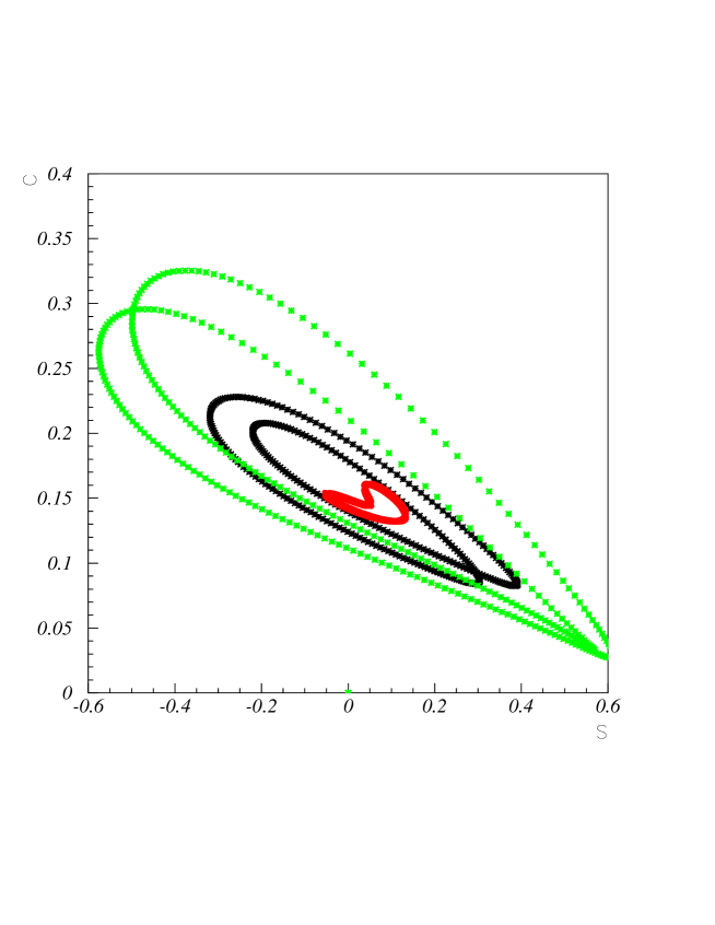
Figure 10: Correlation between $C_{\phi K}$ and $S_{\phi K}$, other parameters are the same with Fig. 9. The outmost two curves correspond to $\mu=m_{b}/2$, the curve in kernel is for $\mu=m_{b}$ and the other two curves are for $\mu=2m_{b}$.

Figs. 5-8 [and also in figs 9-11] are plotted for the case in which the masses of NHBs have large splitting, $m_{A^{0}}=m_{H^{0}}=1$ TeV $\gg m_{h^{0}}=115$ GeV, and consequently $C_{11}(m_{W})$ is the same order of magnitude, compared to $C_{13}(m_{W})$. Now the NHB contributions are as important as those of the charged Higgs boson and $S_{\phi K}$ can reach about $-0.6$, as expected.

In order to demonstrate the NHB contributions, in figures 9-11, we show $S_{\phi K}$ as functions of the phases of $\lambda_{bb}$ and $\lambda_{ss}$, $\theta_{bb}$ and $\theta_{ss}$, and the correlation between $S_{\phi K}$ and $C_{\phi K}$, respectively. It is clear that $S_{\phi K}$ is sensitive to the phases. At the same time, in the range [$-\pi,\pi$] of $\theta_{bb}$ and $\theta_{ss}$ $C_{\phi K}$ changes only several percents. There is a strong correlation between $S_{\phi K}$ and $C_{\phi K}$ and $C_{\phi K}$ is always positive regardless of the sign of $S_{\phi K}$, which is opposite to that of the central value of measurements. Therefore, if the minus $C_{\phi K}$ is confirmed in coming experiments the model III 2HDM could be excluded.

6 Conclusions and Discussions

In summary we have calculated the Wilson coefficients at NLO for the operators in the SM [except for $Q_{7\gamma}$ and $Q_{8g}$], and at LO for the new operators which are induced by NHB penguins in the model III 2HDM. Using the Wilson coefficients obtained, we have calculated the mixing induced time-dependent CP asymmetry $S_{\phi k}$, branching ratio and direct CP asymmetry $C_{\phi K}$ for the decay $B\rightarrow\phi K_{s}$. It is shown that in the reasonable region of parameters where the constraints from $B-\bar{B}$ mixing , $\Gamma(b\to s\gamma)$, $\Gamma(b\to c\tau\bar{\nu}_{\tau})$, $\rho_{0}$, $R_{b}$, $B\to\mu^{+}\mu^{-}$, and electric dipole moments (EDMs) of the electron and neutron are satisfied, the branching ratio of the decay can reach $10\times 10^{-6}$, $C_{\phi K}$ can reach $18\%$ and $S_{\phi k}$ can be negative in quite a large region of parameters and as low as -0.6 in some regions of parameters.

Let us separately discuss the two cases: 1) only the charged Higgs contributions and 2) only the NHB contributions, in addition to the SM ones. Without NHB contributions, i.e., in the first case, the charged Higgs contributions can only decrease $S_{\phi k}$ to around 0. That is, the model III can agree with the present data, $S_{\phi k}=-0.39\pm 0.41$, within $1\sigma$ error.

For the second case, our results show that the effects of NHB induced operators can be sizable even significant, depending on the characteristic scale $\mu$ of the process. Due to the large contributions to the hadronic elements of the operators at the $\alpha_{s}$ order arising from penguin contractions with b quark in the loop, both the Br and $S_{\phi K}$ are sizable or significantly different from those in SM.

Putting all the contributions together, we conclude that the model III can agree with the present data, $S_{\phi k}=-0.39\pm 0.41$, within the $1\sigma$ error. Even if the $S_{\phi k}$ is measured to a level of $-0.4\pm 0.1$ in the future, the model III can still agree with the data at the $2\sigma$ level in quite a large regions of parameters and at the $1\sigma$ level in some regions of parameters. As for $C_{\phi K}$, our result is that it is positive, which is opposite to that of the measured central value. Considering the large uncertainties both theoretically and experimentally at present, we should not take it seriously.

Our results show that both the Br and $S_{\phi k}$ (as well as $C_{\phi K}$) of $B\to\phi K_{S}$ are sensitive to the characteristic scale $\mu$ of the process, as can be seen from eq. (53) and the SM amplitude. The significant scale dependence comes mainly from the $O(\alpha_{s})$ corrections of hadronic matrix elements of the operators $Q_{i}$, i=11,…,16 and also from leading order Wilson coefficients $C_{i}$, i=8g,11,…,16. However, despite there is the scale dependence, the conclusion that the model III can agree with the present data, $S_{\phi k}=-0.39\pm 0.41$, within the $1\sigma$ error can still be drawn definitely.

Note Added

We noticed the reference [26] while completing this work. In the ref. [26] the mixing induced CP asymmetry $S_{\phi K}$ in the model III 2HDM is investigated. Comparing with the paper, our results on the Wilson coefficients of the operators which exist in SM at NLO are in agreement. We differ significantly from the paper in the neutral Higgs boson contributions included. Furthermore, we calculate hadronic matrix elements of operators to the $\alpha_{s}$ order by BBNS’s approach while the paper uses the naive factorization, i.e., at the tree level. Therefore, our numerical results and consequently conclusions are significantly different from those in the paper. Even without including the NHB contributions our results are also different from theirs due to the different precisions of calculating hadronic matrix elements, to which $S_{\phi k}$ is sensitive.

When the publication processing the paper, we were aware of Ref. [27] in which the LO anomalous dimensions for the mixing of $Q_{11,12}$ onto $Q_{3,...,6}$ and $Q_{9}$ are given and those for the mixing of $Q_{13,...,16}$ onto $Q_{7\gamma,8g}$ given in Ref. [28] are confirmed. In this paper these mixings are not taken into account. If including them the numerical results would change but the qualitative features of the results would be the same. We shall include them in a forthcoming paper on“CP asymmetries in $B\to\eta^{\prime}K_{S}$ and $\phi K_{S}$ in a model III 2HDM”.

Figure 1: $S_{\phi K}$ as a function of $\theta\equiv\theta_{bb}+\theta_{tt}$ with $\mu=2m_{b}$ (solid), $m_{b}$ (dashed) and $m_{b}/2$ (dotted), where $m_{H^{\pm}}=$ 200 GeV, $|\lambda_{tt}|=0.03$, $|\lambda_{bb}|=100$, $\lambda_{ss}=\lambda_{cc}=100e^{-i\pi/2}$. The parameter $\xi_{g}$ in neutron EDM expression is 0.03 [14, 25].

Figure 2: $\Delta S$ [defined as difference between $S_{\phi K}$ with and without NHB contributions] as a function of $\theta$ with $\mu=2m_{b}$ (solid), $m_{b}$ (dashed) and $m_{b}/2$ (dotted). Other parameters are the same with Fig. 1.

Figure 3: $C_{\phi K}$ as a function of $\theta$. Other parameters and conventions are the same with Fig. 1.

Figure 4: $\Delta C$ [defined as difference between $C_{\phi K}$ with and without NHB contributions] as a function of $\theta$. Other parameters and conventions are the same with Fig. 3.

Figure 5: $S_{\phi K}$ as a function of $\theta$ with $\mu=2m_{b}$ (solid), $m_{b}$ (dashed) and $m_{b}/2$ (dotted), where $m_{H^{\pm}}=$ 200 GeV, $|\lambda_{tt}|=0.03$, $|\lambda_{bb}|=100$, $\lambda_{ss}=\lambda_{cc}=100e^{-i\pi/2}$. Note that the masses of NHB [in Figs. 5-11] are different with those in Figs. 1-4.

Figure 6: $\Delta S$ as a function of $\theta$ with $\mu=2m_{b}$ (solid), $m_{b}$ (dashed) and $m_{b}/2$ (dotted). Other parameters are the same with Fig. 5.

Figure 7: $C_{\phi K}$ as a function of $\theta$. Other parameters and conventions are the same with Fig. 5.

Figure 8: $\Delta C$ as a function of $\theta$. Other parameters and conventions are the same with Fig. 7.

Figure 9: $S_{\phi K}$ as a function of $\theta_{bb}$ with $\mu=2m_{b}$ (solid), $m_{b}$ (dashed) and $m_{b}/2$ (dotted), where $m_{H^{\pm}}=$ 200 GeV, $|\lambda_{tt}|=0.03$, $|\lambda_{bb}|=100$, $\theta=1.15$ and $\lambda_{cc}=\lambda_{ss}=100e^{i\pi/4}$.

Figure 11: $S_{\phi K}$ as a function of $\theta_{ss}$ with $\mu=2m_{b}$ (solid), $m_{b}$ (dashed) and $m_{b}/2$ (dotted), where $m_{H^{\pm}}=$ 200 GeV, $|\lambda_{tt}|=0.03$, $|\lambda_{ss}|=100$, $\theta=1.15$,$\lambda_{bb}=100e^{-i\pi/4}$ and $\lambda_{cc}=100e^{i\pi/4}$.

References

• [1] Belle Collaboration, hep-ex/0308035.
• [2] See talk given by T. Browder at LP2003,
http://conferences.fnal.gov/lp2003/program/S5/browder_s05_ungarbled.pdf.
• [3] B. Aubert et al.(BABAR Collaboration), hep-ex/0207070.
• [4] T.Β Augshev, talk given at ICHEP 2002 (Belle Collaboration), BELLE-CONF-0232; K. Abe et al., BELLE-CONF-0201 hep-ex/0207098; hep-ex/0212062.
• [5] G. Hamel De Monchenault, hep-ex/0305055.
• [6] K.Β Anikeev et al., arXiv:hep-ph/0201071.
• [7] Y.Β Grossman and M.Β P.Β Worah, Phys.Β Lett.Β B 395, 241 (1997) [arXiv:hep-ph/9612269].
• [8] R.Β Fleischer, Int.Β J.Β Mod.Β Phys.Β A 12, 2459 (1997) [arXiv:hep-ph/9612446].
• [9] D.Β London and A.Β Soni, Phys.Β Lett.Β B 407, 61 (1997) [arXiv:hep-ph/9704277].
• [10] Y.Β Grossman, G.Β Isidori and M.Β P.Β Worah, Phys.Β Rev.Β D 58, 057504 (1998) [arXiv:hep-ph/9708305].
• [11] G.Eigen et al., in Proc. of Snowmass 2001, hep-ph/0112312.
• [12] M.B. Causse, hep-ph/0207070; G. Hiller, hep-ph/0207356; A. Datta, hep-ph/0208016; M. Ciuchini, L. Silvestrini, hep-ph/0208087; S. Khalil and E. Kou, hep-ph/0212023; G.L. Kane et al., hep-ph/0212092; R. Harnik, D.T. Larson and H. Murayama, hep-ph/0212180; S. Khalil and E. Kou, hep-ph/0303214; K. Agashe and C.D. Carone, hep-ph/0304229; D. Chakraverty et al., hep-ph/0306076; hep-ph/0307024; A. Kundu and T. Mitra, Phys. Rev. D67, 116005, (2003); C.Β W.Β Chiang and J.Β L.Β Rosner, Phys.Β Rev.Β D 68, 014007 (2003) [arXiv:hep-ph/0302094].
• [13] J.-F. Cheng, C.-S. Huang and X.-H. Wu, hep-ph/0306086.
• [14] D. Bowser-Chao, K. Cheung, and W.-Y. Keung, Phys. Rev. D59 (1999) 115006 [arXiv:hep-ph/9811235]; Z.Β j.Β Xiao, C.Β S.Β Li and K.Β T.Β Chao, Phys.Β Rev.Β D 62, 094008 (2000), ibid 63, 074005 (2001), ibid 65 114021 (2002); Phys.Β Lett.Β B 473, 148 (2000)
• [15] M. Beneke, G. Buchalla, M. Neubert and C.T. Sachrajda, Nucl. Phys. B606(2001) 245.
• [16] T.P. Cheng and M. Sher, Phys. Rev. D35, 3484 (1987); M. Sher and Y. Yuan, D44, 1461 (1991);
W.S. Hou, Phys. Lett. B296 179 (1992);
A. Antaramian, L. Hall, and A. Rasin, Phys. Rev. Lett. 69, 1871 (1992);
L. Hall and S. Weinberg, Phys. Rev. D48, 979 (1993);
M.J. Savage, Phys. Lett. B266, 135 (1991); L. Wolfenstein and Y.L. Wu, Phys. Rev. Lett. 73 (1994) 2809; D. Atwood, L. Reina, and A. Soni, Phys. Rev. D55, 3156 (1997).
• [17] G.Β Cvetic, C.Β S.Β Kim and S.Β S.Β Hwang, Phys.Β Rev.Β D 58, 116003 (1998) [arXiv:hep-ph/9806282].
• [18] M. Beneke, G. Buchalla, M. Neubert and C.T. Sachrajda, Phys. Rev. Lett. 83(1999) 1914; Nucl. Phys. B591(2000) 313.
• [19] Y.-B. Dai, C.-S. Huang, J.-T. Li, and W.-J. Li, Phys. Rev. D67, 096007 (2003).
• [20] G.Β Buchalla, A.Β J.Β Buras and M.Β E.Β Lautenbacher, Rev.Β Mod.Β Phys.Β  68, 1125 (1996) [arXiv:hep-ph/9512380].
• [21] X.Β G.Β He, J.Β P.Β Ma and C.Β Y.Β Wu, Phys.Β Rev.Β D 63, 094004 (2001) [arXiv:hep-ph/0008159].
• [22] Y.Β Y.Β Keum, H.Β n.Β Li and A.Β I.Β Sanda, Phys.Β Lett.Β B 504, 6 (2001) [arXiv:hep-ph/0004004].
• [23] J.A. Bagger, K.T. Matchev and R.J. Zhang, Phys. Lett. B412(1997) 77; M. Ciuchini et al., Nucl. Phys. B523(1998) 501; C.-S. Huang and Q.-S. Yan, hep-ph/9906493; A.J. Buras, M. Misiak and J. Urban, Nucl.Phys. B586 (2000) 397.
• [24] A.Β L.Β Kagan and M.Β Neubert, Phys.Β Rev.Β D 58, 094012 (1998) [arXiv:hep-ph/9803368].
• [25] I.I. Bigi and N.G. Uraltsev, Nucl. Phys. B353, 321 (1991).
• [26] A.K. Giri and R. Mohanta, hep-ph/0306041.
• [27] G. Hiller and F. Krueger, hep-ph/0310219.
• [28] F. Borzumati et al., Phys. Rev. D62, 075005 (2000).
Refer to caption