Quantum dynamics and thermalization for out-of-equilibrium -theory 111Part of the PhD thesis of S. Juchem
Abstract
The quantum time evolution of -field theory for a spatially homogeneous system in 2+1 space-time dimensions is investigated numerically for out-of-equilibrium initial conditions on the basis of the Kadanoff-Baym equations including the tadpole and sunset self-energies. Whereas the tadpole self-energy yields a dynamical mass, the sunset self-energy is responsible for dissipation and an equilibration of the system. In particular we address the dynamics of the spectral (‘off-shell’) distributions of the excited quantum modes and the different phases in the approach to equilibrium described by Kubo-Martin-Schwinger relations for thermal equilibrium states. The investigation explicitly demonstrates that the only translation invariant solutions representing the stationary fixed points of the coupled equation of motions are those of full thermal equilibrium. They agree with those extracted from the time integration of the Kadanoff-Baym equations for . Furthermore, a detailed comparison of the full quantum dynamics to more approximate and simple schemes like that of a standard kinetic (on-shell) Boltzmann equation is performed. Our analysis shows that the consistent inclusion of the dynamical spectral function has a significant impact on relaxation phenomena. The different time scales, that are involved in the dynamical quantum evolution towards a complete thermalized state, are discussed in detail. We find that far off-shell processes are responsible for chemical equilibration, which is missed in the Boltzmann limit. Finally, we address briefly the case of (bare) massless fields. For sufficiently large couplings we observe the onset of Bose condensation, where our scheme within symmetric -theory breaks down.
pacs:
05.60.+w; 05.70.Ln; 11.10.Wx; 24.10.Cn; 24.10.-i; 25.75.+qI Introduction
Nonequilibrium many-body theory or quantum field theory has become a major topic of research for describing transport processes in nuclear physics, in cosmological particle physics as well as condensed matter physics. The multidisciplinary aspect arises due to a common interest to understand the various relaxation phenomena of quantum dissipative systems. Recent progress in cosmological observations has also intensified the research on quantum fields out-of-equilibrium. Important questions in high-energy nuclear or particle physics at the highest energy densities are: i) how do nonequilibrium systems in extreme environments evolve, ii) how do they eventually thermalize, iii) how phase transitions do occur in real-time with possibly nonequilibrium remnants, and iv) how do such systems evolve for unprecedented short and nonadiabatic timescales?
The very early history of the universe provides scenarios, where nonequilibrium effects might have played an important role, like in the (post-) inflationary epoque (see e.g. inflation ; boya6 ; Linde ), for the understanding of baryogenesis (see e.g. inflation ) and also for the general phenomena of cosmological decoherence (see e.g. GMH93 ). In modern nuclear physics the understanding of the dynamics of heavy-ion collisions at various bombarding energies has always been a major motivation for research on nonequilibrium quantum many-body physics and relativistic quantum field theories, since the initial state of a collision resembles an extreme nonequilibrium situation while the final state might even exhibit a certain degree of thermalization. Indeed, at the presently highest energy heavy-ion collider experiments at RHIC, where one expects to create experimentally a transient deconfined state of matter denoted as quark-gluon plasma (QGP) Mul85 , there are experimental indications – like the build up of collective flow – for an early thermalization accompanied with the build up of a very large pressure. Furthermore, the phenomenon of disoriented chiral condensates (DCC) during the chiral phase transition has lead to a considerable progress for our understanding of nonequilibrium phase transitions at short timescales over the last decade (see e.g. Raja ; Boy95 ; BG97 ). All these examples demonstrate that one needs an ab initio understanding of the dynamics of out-of-equilibrium quantum field theory.
Especially the powerful method of the ‘Schwinger-Keldysh’ Sc61 ; BM63 ; Ke64 ; Cr68 or ‘closed-time-path’ (CTP) (nonequilibrium) real-time Green functions has been shown to provide an appropriate basis for the formulation of the special and complex problems in the various areas of nonequilibrium quantum many-body physics. Within this framework one can then derive and find valid approximations – depending, of course, on the problem under consideration – by preserving overall consistency relations. Originally, the resulting causal Dyson-Schwinger equation of motion for the one-particle Green function (or two-point function), i.e. the Kadanoff-Baym (KB) equations KB , have served as the underlying scheme for deriving various transport phenomena and generalized transport equations. These equations might be considered as an ensemble average over the initial density matrix characterizing the preparation of the initial state of the system, which can be far out of equilibrium. For review articles on the Kadanoff-Baym equations in the various areas of nonequilibrium quantum physics we refer the reader to Refs. DuBois ; dan84a ; Ch85 ; RS86 ; calhu ; Haug . We note in passing, that also the ‘influence functional formalism’ has been shown to be directly related to the KB equations GL98a . Such a relation allows to address inherent stochastic aspects of the latter and also to provide a rather intuitive interpretation of the various self-energy parts that enter the KB equations. The presence of (quantum) noise and dissipation – related by a fluctuation-dissipation theorem – guarantees that the modes or particles of an open system become thermally populated on average in the long-time limit if coupled to an environmental heat bath GL98a .
Furthermore, kinetic transport theory is a convenient tool to study many-body nonequilibrium systems, nonrelativistic or relativistic. Kinetic equations, which do play the central role in more or less all practical simulations, can be derived by means of appropriate KB equations within suitable approximations. Hence, a major impetus in the past has been to derive semi-classical Boltzmann-like transport equations within the standard quasi-particle approximation Ca77 ; Ca78 ; Ca90 . Additionally, off-shell extensions by means of a gradient expansion in the space-time inhomogeneities – as already introduced by Kadanoff and Baym KB – have been formulated: for a relativistic electron-photon plasma BB72 , for transport of electrons in a metal with external electrical field LSV86 , for transport of nucleons at intermediate heavy-ion reactions botmal , for transport of particles in -theory danmrow ; calhu , for transport of electrons in semiconductors SL94 ; Haug , for transport of partons or fields in high-energy heavy-ion reactions Ma95 ; Ge96 ; BD98 ; BI99 , or for a trapped Bose system described by effective Hartree-Fock-Bogolyubov kinetic equations Gri99 . We recall that on the formal level of the KB-equations the various forms assumed for the self-energy have to fulfill consistency relations in order to preserve symmetries of the fundamental Lagrangian knoll1 ; knoll2 ; KB . This allows also for a unified treatment of stable and unstable (resonance) particles. We will shortly come back to this last development.
In nonequilibrium quantum field theory typically the nonperturbative description of (second-order) phase transitions has been in the foreground of interest by means of mean-field (Hartree) descriptions Co94 ; Boy95 ; boya3 ; boya2 ; boya6 ; boya7 , with applications for the evolution of disoriented chiral condensates or the decay of the (oscillating) inflaton in the early reheating era. ‘Effective’ mean-field dissipation (and decoherence) – solving the so-called ‘backreaction’ problem – was incorporated by particle production through order parameters explicitly varying in time. However, it had been then realized that such a dissipation mechanism, i.e. transferring collective energy from the time-dependent order parameter to particle degrees of freedom, can not lead to true dissipation and thermalization. Such a conclusion has already been known for quite some time within the effective description of heavy-ion collisions at low energy. Full time-dependent Hartree or Hartree-Fock descriptions negele were insufficient to describe the reactions with increasing collision energy; additional Boltzmann-like collision terms had to be incorporated in order to provide a more adequate description of the collision processes.
The incorporation of true collisions then has been formulated also for the various quantum field theories boya1 ; boya4 ; boya5 ; CH02 . Here, a systematic 1/N expansion of the ‘2PI effective action’ is conventionally invoked calhu ; Co94 ; CH02 serving as a nonperturbative expansion parameter. Of course, only for large N this might be a controlled expansion. In any case, the understanding and the influence of dissipation with the chance for true thermalization – by incorporating collisions – has become a major focus of recent investigations. The resulting equations of motion always do resemble the KB equations; in their general form (beyond the mean-field or Hartree(-Fock) approximation) they do break time invariance and thus lead to irreversibility. This macroscopic irreversibility arises from the truncations of the full theory to obtain the self-energy operators in a specific limit. As an example we mention the truncation of the (exact) Martin-Schwinger hierarchy in the derivation of the collisional operator in Ref. botmal or the truncation of the (exact) BBGKY hierarchy in terms of n-point functions botmal ; SKK03 ; andy ; Wang ; Peter ; Peter2 ; Peter3 ; Haus98 .
In principle, the nonequilibrium quantum dynamics is nonperturbative in nature. Unphysical singularities only appear in a limited truncation scheme, e.g. ill-defined pinch singularities AS94 , which do arise at higher order in a perturbative expansion in out-of-equilibrium quantum field theory, are regularized by a consistent nonperturbative description (of Schwinger-Dyson type) of the nonequilibrium evolution, since the resummed propagators obtain a finite width GL99 . Such a regularization is also observed by other resummation schemes like the dynamical renormalization group technique developed recently boya5 .
Although the analogy of KB-type equations to a Boltzmann-like process is quite obvious, this analogy is far from being trivial. The full quantum formulation contains much more information than a semi-classical (generally) on-shell Boltzmann equation. The dynamics of the spectral (i.e. ‘off-shell’) information is fully incorporated in the quantum dynamics while it is missing in the Bolzmann limit. A full answer to the question of quantum equilibration can thus only be obtained by a detailed numerical solution of the quantum description itself. This is the basic aim of our present study.
Before pointing out the scope of the present paper, we briefly address previous works that have investigated numerically approximate or full solutions of KB-type equations. A seminal work has been carried out by Danielewicz dan84b , who investigated for the first time the full KB equations for a spatially homogeneous system with a deformed Fermi sphere in momentum space for the initial distribution of occupied momentum states in order to model the initial condition of a heavy-ion collision in the nonrelativistic domain. In comparison to a standard on-shell semi-classical Boltzmann equation the full quantum Boltzmann equation showed quantitative differences, i.e. a larger collective relaxation time for complete equilibration of the momentum distribution . This ‘slowing down’ of the quantum dynamics was attributed to quantum interference and off-shell effects. Similar quantum modifications in the equilibration and momentum relaxation have been found in Ca77 and for a relativistic situation in Ref. CGreiner . Particular emphasis was put in this study CGreiner ; CGreinera on non-local aspects (in time) of the collision process and thus the potential significance of memory effects on the nuclear dynamics. In the following, full and more detailed solutions of nonrelativistic KB equations have been performed by Köhler koe1 ; koe2 with special emphasis on the build up of initial many-body correlations on short time scales. Moreover, the role of memory effects has been clearly shown experimentally by femtosecond laser spectroscopy in semiconductors Haug95 in the relaxation of excitons. Solutions of quantum transport equations for semiconductors Haug ; WJ99 – to explore relaxation phenomena on short time and distance scales – have become also a very active field of research.
In the last years the numerical treatment of general quantum dynamics out-of-equilibrium, as described within 2PI effective action approaches at higher order, have become more frequent berges1 ; berges2 ; berges3 ; CDM02 ; berges4 . The subsequent equations of motion are very similar to the KB equations, although more involved expressions for a non-local vertex function – as obtained by the 2PI scheme – are taken care of. The numerical solutions are also obtained for homogeneous systems, only. The studies in Refs. berges1 ; berges2 ; berges3 ; CDM02 have investigated the situation in 1+1 dimensions for -theory, the last work CDM02 also for non-symmetric configurations exploring the nonequilibrium dynamics of a phase transition. In general, all studies do demonstrate that the system eventually shows equilibration in the momentum occupation. The situation in 1+1 dimensions, however, is a rather unrealistic case as on-shell 2-to-2 elastic collisions are strictly forward and thus can not contribute at all to equilibration in momentum space. The time scales found in Refs. berges1 ; berges2 ; berges3 for thermalization are thus a delicate higher order off-shell effect. Very recently, a study in 3+1 dimensions berges4 , treating spherical symmetric distributions of momentum excitations for a coupled fermion-boson Yukawa-type system, has shown equilibration and thermalization in the fermionic as well as bosonic momentum occupation at the same temperature. Still, again, a detailed and quantitative interpretation of the time scales found was not given.
As already stressed, in the present study we will focus in particular on the full quantum dynamics of the spectral (i.e. ‘off-shell’) information contained in the nonequilibrium single-particle spectral function. A first discussion of this issue has previously been given in berges2 by Berges and Aarts. Here we want to show, by using the spectral representation, how complete thermalization of all single-particle quantum fluctuations will be approached. In addition, the quantum dynamics of the spectral function is also a lively discussed issue in the microscopic modeling of hadronic resonances with a broad mass distribution. This is of particular relevance for simulations of heavy-ion reactions HHab ; EBM99 ; knoll3 ; caju1 ; caju2 ; caju3 ; Leupold ; CB99 , where e.g. the -resonance or the -meson already show a large decay width in vacuum. Especially the vector meson is a promising hadronic particle for showing possible in-medium modifications in hot and compressed nuclear matter (see e.g. RW00 ; CB99 ), since the leptonic decay products are of only weakly interacting electromagnetic nature. Indeed, the CERES experiment CERES at the SPS at CERN has found a significant enhancement of lepton pairs for invariant masses below the pole of the -meson, giving evidence for such modifications. Hence, a consistent formulation for the transport of extremely short-lived particles beyond the standard quasi-particle approximation is needed. On the one side, there exist purely formal developments starting from a first-order gradient expansion of the underlying KB equations HHab ; knoll3 ; Leupold , while on the other side already first practical realizations for various questions have emerged EBM99 ; caju1 ; caju2 ; caju3 ; cas03 . The general idea is to obtain a description for the propagation of the off-shell mass squared . A fully ab initio investigation, however, without any further approximations, does not exist so far.
Our work is organized as follows: In Section II we will present the relevant equations for the nonequilibrium dynamics in case of the -theory, i.e. briefly derive the Kadanoff-Baym equations of interest. Section III is devoted to first numerical studies on equilibration phenomena and separation of time scales employing different initial configurations. The actual numerical algorithm used is described in Appendix A as well as the renormalization by counterterms in Appendix B in order to achieve ultraviolet convergent results. The individual phases of the quantum evolution are analyzed in more detail in Section IV, i.e. the initial build up of correlations, the time evolution of the spectral functions and the approach to chemical equilibrium. Furthermore, it is shown that the solutions of the Kadanoff-Baym equations for yield the proper off-shell thermal state, i.e. the Green functions fulfill the Kubo-Martin-Schwinger (KMS) relation in the long time limit. Section V concentrates on approximate dynamical schemes, in particular the well-known Boltzmann limit. The solutions of the latter limit as well as from a simple relaxation approximation will be confronted with the numerical results from the Kadanoff-Baym equations. We close this work in Section VI with a summary of our findings and a brief presentation of the results for massless Bose fields. Appendix C discusses the most general choices for the initial conditions of the Kadanoff-Baym equations. Furthermore, in Appendix D we will present an efficient method for the calculation of the self-consistent resummed spectral function in thermal equilibrium for the present field theory, while Appendix E addresses the stationary solution of the Boltzmann limit.
II Nonequilibrium dynamics for -theory
The scalar -theory is an example for a fully relativistic
field theory of interacting scalar particles that allows to test
theoretical approximations
Peter ; Peter2 ; Peter3 ; berges1 ; berges2 ; berges3
without coming to the problems of gauge-invariant truncation schemes
Haus98 .
Its Lagrangian density is given by
| (1) |
where denotes the ‘bare’ mass and is the coupling constant determining the interaction strength of the scalar fields.
II.1 The Kadanoff-Baym equations
As mentioned in the Introduction, a natural starting point for
nonequilibrium theory is provided by the closed-time-path (CTP)
method. Here all quantities are given on a special real-time
contour with the time argument running from to
on the chronological branch and returning from to
on the antichronological branch . In cases of
systems prepared at time this value is (instead of
) the start and end point of the real-time contour. In
particular the path-ordered Green functions are defined as
where the operator orders the field operators according to the position of their arguments on the real-time path as accomplished by the path step-functions . The expectation value in (II.1) is taken with respect to some given density matrix , which is constant in time, while the operators in the Heisenberg picture contain the whole information of the time dependence of the nonequilibrium system.
Self-consistent equations of motion for these Green functions can
be obtained with help of the two-particle irreducible (2PI)
effective action . It is given by the Legendre
transform of the generating functional of the connected Green
functions as
| (3) |
in case of vanishing vacuum expectation value
knoll1 . In (3)
depends only on free Green functions and is treated as
a constant with respect to variation, while the symbols
represent convolution integrals over the closed-time-path with the
contour specified above.
The functional is the sum of all closed 2PI
diagrams built up by full propagators ; it determines the
self-energies by functional variation as
| (4) |
From the effective action (3) the equations of motion
for the Green function are obtained by the stationarity condition
| (5) |
giving the Dyson-Schwinger equation for the full path-ordered
Green function as
| (6) |
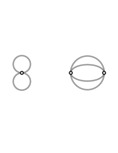
In our present calculation we take into account contributions up
to the three-loop order for the -functional
(cf. Fig. 1), which reads explicitly
| (7) |
where denotes the spatial dimension of the problem ( in the case considered below).
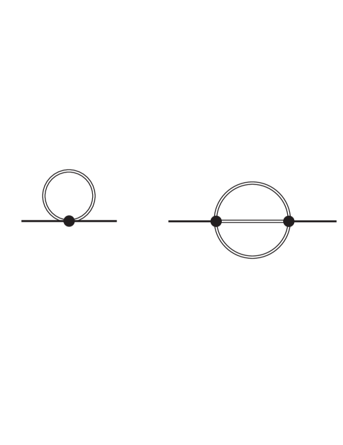
This approximation corresponds to a weak coupling expansion such that we consider contributions up to the second superficial order in the coupling constant (cf. Fig. 2). For the superficial coupling constant order we count the explicit coupling factors associated with the visible vertices. The hidden dependence on the coupling strength – which is implicitly incorporated in the self-consistent Green functions that build up the -functional and the self-energies – is ignored on that level. For our present purpose this approximation is sufficient since we include the leading mean-field effects as well as the leading order scattering processes that pave the way to thermalization.
For the actual calculation it is advantageous to change to a
single-time representation for the Green functions and
self-energies defined on the closed-time-path. In line with
the position of the coordinates on the contour there exist
four different two-point functions
| (8) | |||||
Here represent the (anti-)time-ordering operators in case of both arguments lying on the (anti-)chronological branch of the real-time contour. These four functions are not independent of each other. In particular the non-continuous functions and are built up by the Wightman functions and and the usual -functions in the time coordinates. Since for the real boson theory (1) the relation holds (8), the knowledge of the Green functions for all characterizes the system completely. Nevertheless, we will give the equations for and explicitly since this is the familiar representation for general field theories danmrow .
By using the stationarity condition for the action
(5) and resolving the time structure of the path
ordered quantities in the Dyson-Schwinger equation (6)
we obtain the Kadanoff-Baym equations for the
time evolution of the Wightman functions danmrow ; berges1 :
Here the path-ordered self-energy has been divided into a local
contribution and a non-local one, which can be
expressed – analogously to the Green functions (II.1) –
by a sum over path -functions.
The self-energy entering the Dyson-Schwinger equation
(6) thus is written as
| (10) |
Within the three-loop approximation for the 2PI effective action
(i.e. the -functional (7))
we get two different self-energies:
In leading order of the coupling constant only the local tadpole diagram
(l.h.s. of Fig. 2) contributes and leads to the
generation of an effective mass for the field quanta. This
self-energy (in coordinate space) is given by
| (11) |
In next order in the coupling constant (i.e. )
the non-local sunset self-energy (r.h.s. of Fig. 2)
enters the time evolution as
| (12) |
Thus the Kadanoff-Baym equation (II.1) in our case includes the influence of a mean-field on the particle propagation – generated by the tadpole diagram – as well as scattering processes as inherent in the sunset diagram.
The Kadanoff-Baym equation (II.1) describes the full quantum nonequilibrium time evolution on the two-point level for a system prepared at an initial time , i.e. when higher order correlations are discarded. The causal structure of this initial value problem is obvious since the time integrations are performed over the past up to the actual time (or , respectively) and do not extend to the future.
Furthermore, also linear combinations of the Green functions in
single time representation are of interest.
The retarded Green function and the advanced Green function
are given as
| (13) | |||||
| (14) | |||||
These Green functions contain exclusively spectral, but no statistical
information of the system.
Their time evolution is given by
| (15) | |||||
| (16) |
where the retarded and advanced self-energies , are defined via , similar to the Green functions (13) and (14). Thus the retarded (advanced) Green functions are determined by retarded (advanced) quantities, only.
II.2 Homogeneous systems in space
In the following we will restrict to homogeneous systems in space.
To obtain a numerical solution the Kadanoff-Baym equation
(II.1) is transformed to momentum space:
where we have summarized both memory integrals into the function . The equation of motion in the second time direction is given analogously.
In two-time and momentum space ()
representation the self-energies in (II.2) read
| (18) | |||||
For the numerical solution of the Kadanoff-Baym equations (II.2) we have developed a flexible and accurate algorithm, which is described in more detail in Appendix A. Furthermore, a straightforward integration of the Kadanoff-Baym equations (II.2) in time does not lead to meaningful results since in 2+1 space-time dimensions both self-energies (18,II.2) are ultraviolet divergent. We note, that due to the finite mass adopted in (1) no problems arise from the infrared momentum regime. The ultraviolet regime, however, has to be renormalized by introducing proper counterterms. The details of the renormalization scheme are given in Appendix B as well as a numerical proof for the convergence in the ultraviolet regime.
III First numerical studies on equilibration
In the following Sections we will use the renormalized mass = 1, which implies that times are given in units of the inverse mass or is dimensionless. Accordingly, the coupling in (1) is given in units of the mass such that is dimensionless, too.
As already observed in the 1+1 dimensional case berges3 the mean-field term, generated by the tadpole diagram, does not lead to an equilibration of arbitrary initial momentum distributions since it only modifies the propagation of the particles by the generation of an effective mass. Our calculations lead to the same findings and thus we skip an explicit presentation of the actual results. Accordingly, thermalization in 2+1 dimensions requires the inclusion of the collisional self-energies as generated by the sunset diagram. All calculations to be shown in the following consequently involve both self-energies.
III.1 Initial conditions
In order to investigate equilibration phenomena on the basis of
the Kadanoff-Baym equations for our 2+1 dimensional problem, we
first have to specify the initial conditions for the time
integration.
This is a problem of its own and discussed in more detail in
Appendix C.
For our present study we consider four different initial
distributions that are all characterized by the same energy
density (see Section IV.1 for an explicit representation).
Consequently, for large times () all
initial value problems should lead to the same equilibrium final
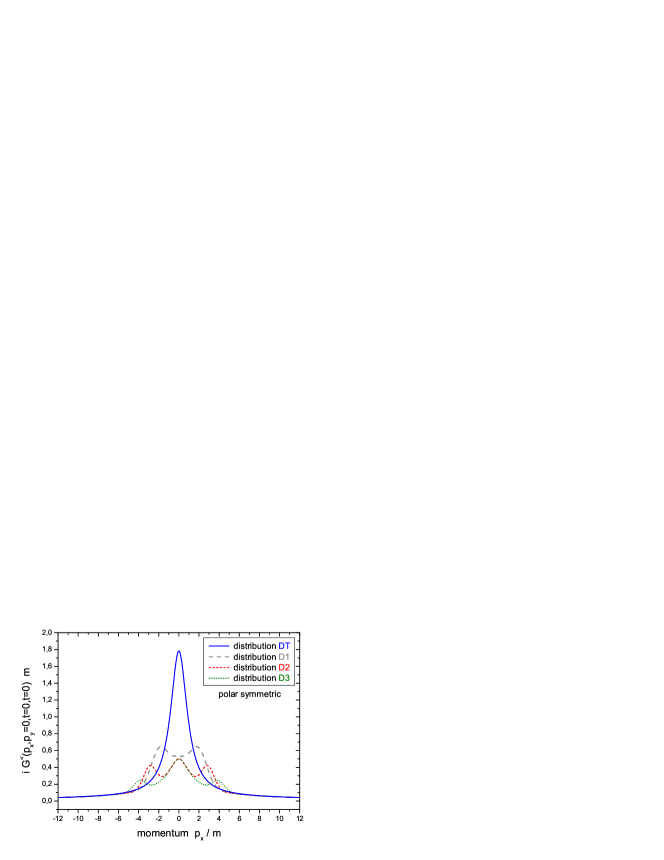
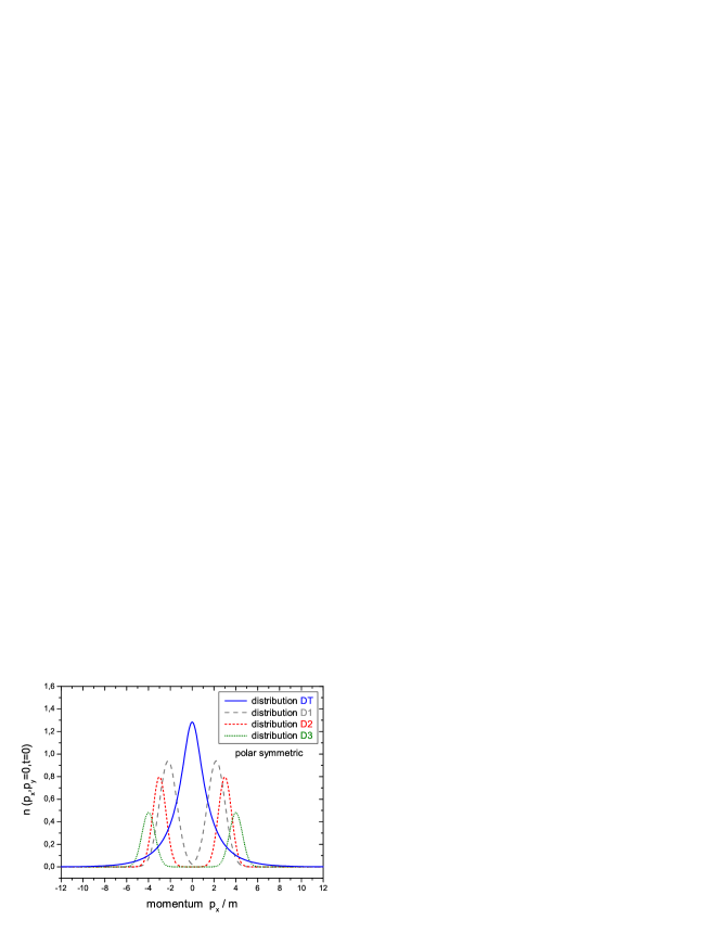
state. The initial equal-time Green functions
adopted are displayed in
Fig. 3 (upper part) as a function of the momentum
(for ).
We concentrate here on polar symmetric configurations due to the large
numerical expense for this first investigation222In Section
V we will present also calculations for non-symmetric systems..
Since the equal-time Green functions
are
purely imaginary, we show only the real part of in
Fig. 3.
Furthermore, the corresponding initial distribution functions in
the occupation density , related to
via
| (20) |
are shown in Fig. 3 in the lower part. For an explicit representation of the other Green functions , and (cf. Appendix A) at initial time we refer to the discussion of the general initial conditions in Appendix C. While the initial distributions D1, D2, D3 have the shape of (polar symmetric) ‘tsunami’ waves boya7 with maxima at different momenta in , the initial distribution DT corresponds to a free Bose gas at a given initial temperature that is fixed by the initial energy density. According to (20) the difference between the Green functions and the distribution functions is basically given by the vacuum contribution, which has its maximum at small momenta. Thus even for the distributions D1, D2, D3 the corresponding Green functions are non-vanishing for 0.
Since we consider a finite volume we work in a basis of momentum modes characterized by the number of nodes in each direction. The number of momentum modes is typically in the order of 40; we checked that all our results are stable with respect to an increasing number of basis states and do not comment on this issue any more, since this is a strictly necessary condition for our analysis. For times we consider the systems to be noninteracting and switch on the interaction () for to explore the quantum dynamics of the interacting system for .
We directly step on with the actual numerical results.
III.2 Equilibration in momentum space
The time evolution of various (selected) momentum modes of the equal-time Green function for the different initial states D1, D2, D3 and DT is shown in Fig. 4, where the dimensionless time is displayed on a logarithmic scale.
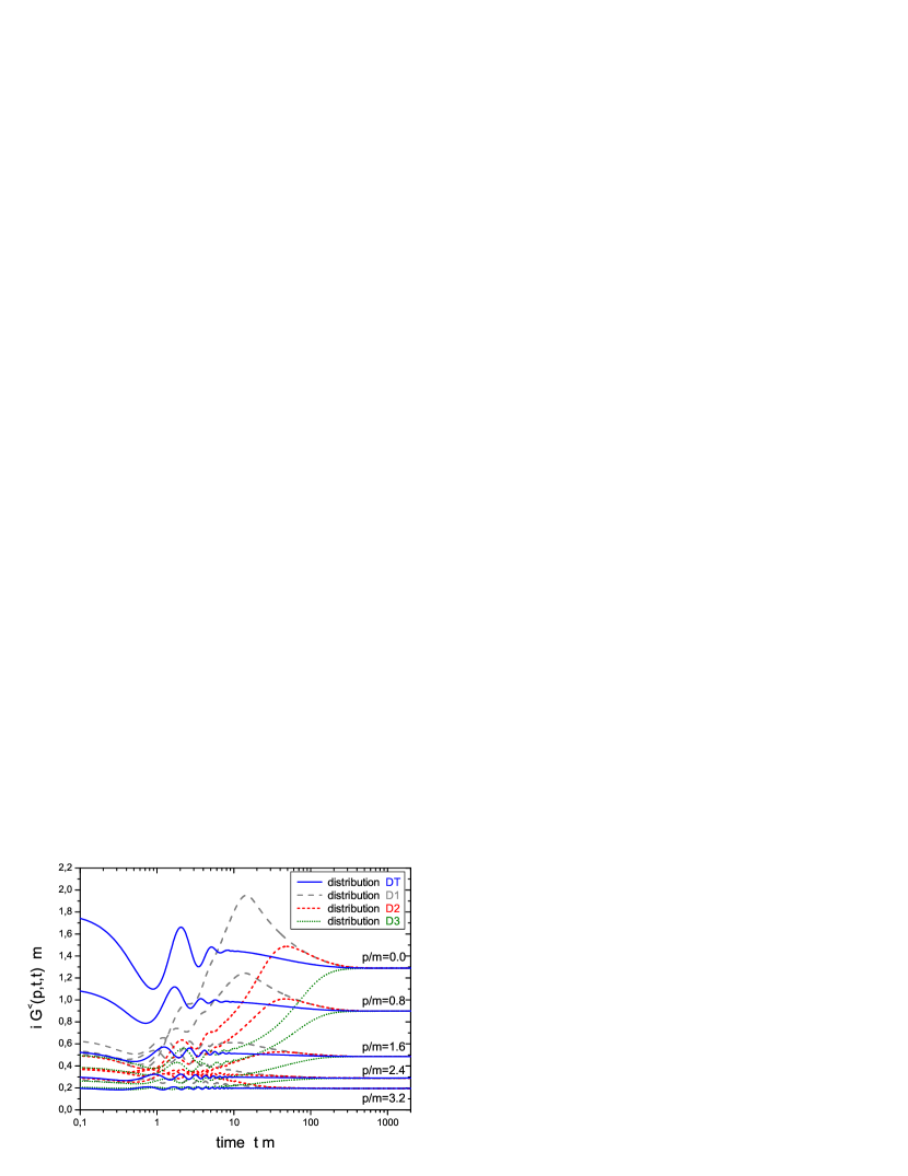
We observe that starting from very different initial conditions – as introduced in Fig. 3 – the single momentum modes converge to the same respective numbers for large times as characteristic for a system in equilibrium. As noted above, the initial energy density is the same for all distributions and energy conservation is fulfilled strictly in the time integration of the Kadanoff-Baym equations. The different momentum modes in Fig. 4 typically show a three-phase structure. For small times () one finds damped oscillations that can be identified with a typical switching on effect at , where the system is excited by a sudden increase of the coupling constant to . Here dephasing and relaxation of the initial conditions happen on a time scale of the inverse damping rate (cf. Appendix C) . We note in passing that one might also start with an effective initial mass including the self-consistent tadpole contribution berges3 , however, our numerical solutions showed no significant difference for the equilibration process such that we discard an explicit representation. The damping of the initial oscillations depends on the coupling strength and is more pronounced for strongly coupled systems.
For ‘intermediate’ time scales () one observes a strong change of all momentum modes in the direction of the final stationary state. We address this phase to ‘kinetic’ equilibration and point out, that – depending on the initial conditions and the coupling strength – the momentum modes can temporarily even exceed their respective equilibrium value. This can be seen explicitly for the lowest momentum modes ( or ) of the distribution D1 (long dashed lines) in Fig. 4, which possesses initially maxima at small momentum. Especially the momentum mode of the equal-time Green function , which starts at around 0.52, is rising to a value of 1.95 before decreasing again to its equilibrium value of 1.29. Thus the time evolution towards the final equilibrium value is – after an initial phase with damped oscillations – not necessarily monotonic. For different initial conditions this behaviour may be weakened significantly as seen for example in case of the initial distribution D2 (short dashed lines) in Fig. 4. Coincidently, both calculations D1 and D2 show approximately the same equal-time Green function values for times . Note, that for the initial distribution D3 (dotted lines) the non-monotonic behaviour is not seen any more.
In general, we observe that only initial distributions (of the well type) show this feature during their time evolution, if the maximum is located at sufficiently small momenta. Initial configurations like the distribution DT (solid lines) – where the system initially is given by a free gas of particles at a temperature – do not show this property. We also remark that this behaviour of ‘overshooting’ – as in the particular case of D1 – is not observed in a simulation with a kinetic Boltzmann equation (see Appendix E). Hence this highly nonlinear effect must be attributed to quantal off-shell and memory effects not included in the standard Boltzmann limit. Although the DT distribution is not the equilibrium state of the interacting theory, the actual numbers are much closer to the equilibrium state of the interacting system than the initial distributions D1, D2 and D3. Therefore, the evolution for DT proceeds less violently. We point out, that in contrast to the calculations performed for -theory in 1+1 space-time dimensions berges3 we find no power law behaviour for intermediate time scales.
The third phase, i.e. the late time evolution () is characterized by a smooth approach of the single momentum modes to their respective equilibrium values. As we will see in Section IV.4 this phase is adequately characterized by chemical equilibration processes.
The three phases addressed in context with Fig. 4 will be investigated and analyzed in more detail in the following Section.
IV The different phases of quantum equilibration
IV.1 Build up of initial correlations
The time evolution of the interacting system within the standard
Kadanoff-Baym equations is characterized by the build up of early
correlations. This can be seen from Fig. 5 where
all contributions to the energy density knoll1
are displayed separately as a function of time with the initial value
at subtracted.
The kinetic energy density
is represented by all parts of
that are independent of the coupling constant
(). All terms proportional to are
summarized by the tadpole energy density
including the actual tadpole term as well as the corresponding
tadpole mass counterterm (cf. Appendix B).
The contributions from
the sunset diagram – again given by the
correlation integral as well as by the sunset mass counterterm
(cf. Appendix B) – are represented by the sunset energy density
.
| (21) | |||||
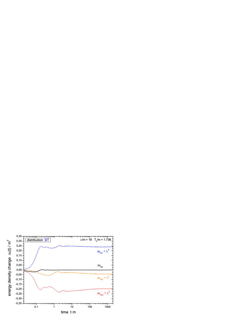
The calculation in Fig. 5 has been performed for the initial distribution DT (which represents a free gas of Bose particles at temperature ) with a coupling constant of . This state is stationary in the well-known Boltzmann limit (cf. Section V), but it is not for the Kadanoff-Baym equation. In the full quantum calculations the system evolves from an uncorrelated initial state and the correlation energy density decreases rapidly with time. The decrease of the correlation energy which is – with exception of the sunset mass counterterm contribution – initially zero is approximately compensated by an increase of the kinetic energy density . Since the kinetic energy increases in the initial phase, the final temperature is slightly higher than the initial ‘temperature’ . The remaining difference is compensated by the tadpole energy density such that the total energy density is conserved.
While the sunset energy density and the kinetic energy density always show a time evolution comparable to Fig. 5, the change of the tadpole energy density depends on the initial configuration and may be positive as well. Since the self-energies are obtained within a -derivable scheme the fundamental conservation laws, as e.g. energy conservation, are respected to all orders in the coupling constant. When neglecting the sunset contributions and starting with a non-static initial state of identical energy density one observes the same compensating behaviour between the kinetic and the tadpole terms.
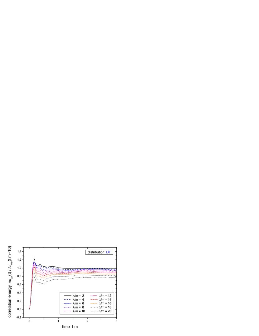
From Fig. 5 one finds that the system correlates in a very short time () in comparison to the time for complete equilibration. The time to build up the correlations is rather independent of the interaction strength as seen from Fig. 6, where calculations with the same initial state DT are compared for several coupling constants in steps of 2. For all couplings the change of the correlation energy density here has been normalized to the asymptotic correlation strength (). Fig. 6 shows that the correlation time (which we define by the position of the first maximum) is approximately the same for all coupling constants. Within our definition the correlation time is for all couplings . This result is in line with the KB studies of nonrelativistic nuclear matter problems, where the same independence from the coupling strength has been observed for the correlation time koe2 . A similar result has, furthermore, been obtained within the correlation dynamical approach of Ref. andy . Thus quantum systems apparently correlate on time scales that are very short compared to ‘kinetic’ or ‘chemical’ equlibration time scales.
The question now arises how such short time scales come about.
We recall, that equations of motion containing memory integrals,
like the Kadanoff-Baym equations, are the inevitable result of a reduction
of multi-particle dynamics to the one-body level which induces
phase correlations into the history of the system FS90 ; RM96 .
This is similar to the situation encountered in the derivation of
the standard Boltzmann equation, which only holds if one can separate
between two time scales, (relaxation time scale),
distinguishing between rapidly changing (‘irrelevant’) observables and
smoothly behaving (‘relevant’) observables.
Indeed, it had been shown for a nucleonic system CGreinera
that such a finite memory in the collision process may have a profound
influence on thermalization for medium-energy nuclear reactions.
In any case, a finite correlation time is generated
by first a constructive and then destructive interference
of the various scattering channels building up for times going more
and more in the past.
For a fermionic system typical memory kernels for the collision integral
are given in Refs. CGreiner ; CGreinera ; koe1 ).
The structure of such memory kernels is governed by the off-shell
behaviour and the phase-space average of the two-particle
scattering amplitude, i.e.
| (22) |
Of present concern is now the formation of the correlation
energy and not the memory kernels of the collisional integrals,
although they are closely related.
The explicit correlation part of contains the
momentum integral over the function , which itself
is given by a memory integral over time as stated in (A)
in Appendix A.
From the explicit expression one notices that
and for small times builds up
coherently by the various ‘scattering’ contributions.
For a fermionic system describing cold nuclear matter, similar
expressions for the collisional energy density have been found and
analyzed in detail by Köhler and Morawetz koe2 .
It has been found, that the time to build up correlation energy by
collisions from an initially uncorrelated system is given by
, where denotes the Fermi
energy.
The memory integrals of – or those entering the quantal transport
equations – can also contain classical contributions.
For a dilute and equilibrated Maxwell-Boltzmann gas of nonrelativsitic
particles at finite temperature and assuming a static, Gaussian
interaction potential , the various kernels
can be worked out analytically dan84a ; RM96 ; koe2 .
The correlation time is then given by
| (23) |
The first part reflects the intuitive expectation, i.e. the time a classical particle passes through the range of a potential; the second part reflects the average temporal extent associated with the time-energy uncertainty relation induced by the characteristic (off-shell) energy scale in a typical collision. For our present situation, i.e. a relativistic bosonic theory interacting via a 4-point coupling, the temperature defines the only scale. Hence, , which is a pure quantal effect. This estimate is in agreement with our numerical findings.
IV.2 Time evolution of the spectral function
Within the Kadanoff-Baym calculations the full quantum information
of the two-point functions is retained. Consequently, one has
access to the spectral properties of the nonequilibrium system
during its time evolution.
A similar study has been carried out for 1+1 dimensions in Ref. berges2 .
The spectral function for the present settings is given by
| (24) |
From our dynamical calculations the spectral function in
Wigner space for each system time is
obtained via Fourier transformation with respect to the relative
time coordinate :
| (25) |
We note, that a damping of the function in
relative time corresponds to a finite width
of the spectral function in Wigner space. This width in turn can
be interpreted as the inverse life time of the interacting scalar
particle. We recall, that the spectral function –
for all times and for all momenta –
obeys the normalization
| (26) |
which is nothing but a reformulation of the equal-time commutation relation.
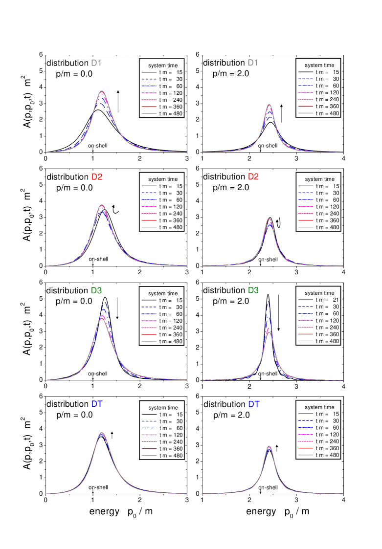
In Fig. 7 we display the time evolution of the spectral function for the initial distributions D1, D2, D3 and DT for two different momentum modes and . Since the spectral functions are antisymmetric in energy for the momentum symmetric configurations considered, i.e. , we only show the positive energy part. For our initial value problem in two-times and momentum space the Fourier transformation (25) is restricted for system times to an interval . Thus in the very early phase the spectral function assumes a finite width already due to the limited support of the Fourier transform in the time interval and a Wigner representation is not very meaningful. We, therefore, present the spectral functions for various system times starting from up to .
For the free thermal initialization DT the evolution of the spectral function is very smooth and comparable to the smooth evolution of the equal-time Green function as discussed in Section III. In this case the spectral function is already close to the equilibrium shape at small times being initially only slightly broader than for late times. The maximum of the spectral function (for all momenta) is higher than the (bare) on-shell value and nearly keeps its position during the whole time evolution. This results from a positive tadpole mass shift, which is only partly compensated by a downward shift originating from the sunset diagram.
The time evolution for the initial distributions D1, D2 and D3 has a richer structure. For the distribution D1 the spectral function is broad for small system times (see the line for ) and becomes a little sharper in the course of the time evolution (as presented for the momentum mode as well as for ). In line with the decrease in width the height of the spectral function is increasing (as demanded by the normalization property (26)). This is indicated by the small arrow close to the peak position. Furthermore, the maximum of the spectral function (which is approximately the on-shell energy) is shifted slightly upwards for the zero mode and downwards for the mode with higher momentum. Although the real part of the (retarded) sunset self-energy leads (in general) to a lowering of the effective mass, the on-shell energy of the momentum modes is still higher than the one for the initial mass (indicated by the ‘on-shell’ arrow) due to the positive mass shift from the tadpole contribution.
For the initial distribution D3 we find the opposite behaviour. Here the spectral function is quite narrow for early times and increases its width during the time evolution. Correspondingly, the height of the spectral function decreases with time. This behaviour is observed for the zero momentum mode as well as for the finite momentum mode . Especially in the latter case the width for early times is so small that the spectral function shows oscillations originating from the finite range of the Fourier transformation from relative time to energy. Although we have already increased the system time for the first curve to (for the oscillations are much stronger) the spectral function is not fully resolved, i.e. it is not sufficiently damped in relative time in the interval available for the Fourier transform. For later times the oscillations vanish and the spectral function tends to the common equilibrium shape.
The time evolution of the spectral function for the initial distribution D2 is in between the last two cases. Here the spectral function develops (at intermediate times) a slightly higher width than in the beginning before it is approaching the narrower static shape again. The corresponding evolution of the maximum is again indicated by the (bent) arrow. Finally, all spectral functions show the (same) equilibrium form represented by the solid gray line.
As already observed in Section III for the equal-time Green functions, we emphazise, that there is no unique time evolution for the nonequilibrium systems. In fact, the evolution of the system during the equilibration process depends on the initial conditions. Our findings are slightly different from the conclusions drawn in berges2 stating that the Wigner transformed spectral function is slowly varying, which might be due to the lower dimension. Still the time dependence of the spectral function is moderate enough, such that one might also work with some time-averaged or even the equilibrium spectral function. In order to investigate this issue in more quantitative detail, we concentrate on the maxima and widths of the spectral functions in the following.
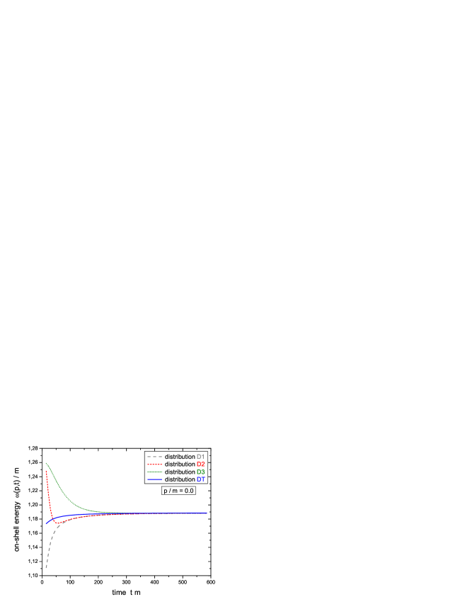
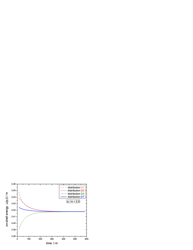
Since the solution of the Kadanoff-Baym equation provides the full spectral information for all system times the evolution of the on-shell energies can be studied as well as the spectral widths. In Fig. 8 we display the time dependence of the on-shell energies – defined by the maximum of the spectral function – of the momentum modes (l.h.s.) and (r.h.s.) for the four initial distributions D1, D2, D3 and DT. We see that the on-shell energy for the zero momentum mode increases with time for the initial distribution D1 and to a certain extent for the free thermal distribution DT (as can be also extracted from Fig. 7). The on-shell energy of distribution D3 shows a monotonic decrease during the evolution while it passes through a minimum for distribution D2 before joining the line for the initialization D1. For momentum a rather opposite behaviour is observed. Here the on-shell energy for distribution D1 (and less pronounced for the distribution DT) are reduced in time whereas it is increased in the case of D3. The result for the initialization D2 is monotonous for this mode and matches the one for D1 already for moderate times. Thus we find, that the time evolution of the on-shell energies does not only depend on the initial conditions, but might also be different for various momentum modes. It turns out – for the initial distributions investigated – that the above described characteristics change around and are retained for larger momenta (not presented here).
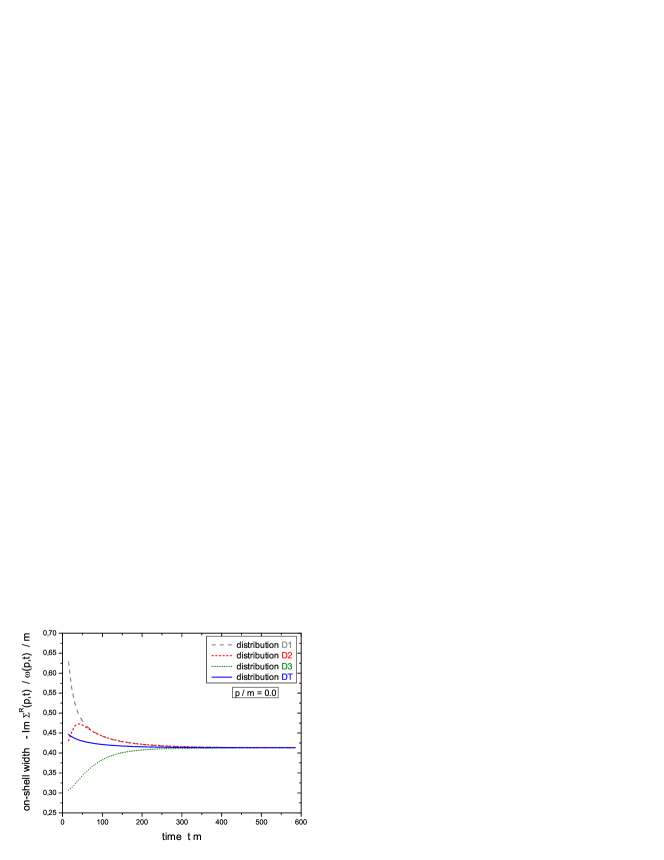
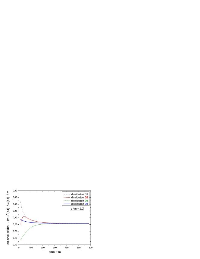
Furthermore, we show in Fig. 9 the time
evolution of the on-shell width for the usual momentum modes and
different initial distributions. The on-shell width
is given by the imaginary part of the retarded sunset self-energy
at the on-shell energy of each respective momentum mode as
| (27) |
As already discussed in connection with Fig. 7 we observe for both momentum modes a strong decrease of the on-shell width for the initial distribution D1 (long dashed lines) associated with a narrowing of the spectral function. In contrast, the on-shell widths of distribution D3 (dotted lines) increase with time such that the corresponding spectral functions broaden towards the common stationary shape. For the initialization D2 (short dashed lines) we observe a non-monotonic evolution of the on-shell widths connected with a broadening of the spectral function at intermediate times. Similar to the case of the on-shell energies we find, that the results for the on-shell widths of the distributions D1 and D2 coincide well above a certain system time. As expected from the lower plots of Fig. 7, the on-shell width for the free thermal distribution DT (solid lines) exhibits only a weak time dependence with a slight decrease in the initial phase of the time evolution.
In summarizing this subsection we point out, that there is no universal time evolution of the spectral functions for the initial distributions considered. Peak positions and widths depend on the initial configuration and evolve differently in time. However, we find only effects in the order of 10% for the on-shell energies in the initial phase of the system evolution and initial variations of 50% for the widths of the dominant momentum modes. Thus, depending on the physics problem of interest, one might eventually discard an explicit time dependence of the spectral functions and adopt the equilibrium shape.
IV.3 The equilibrium state
In Section III we have seen that arbitrary initial momentum configurations of the same energy density approach a stationary limit for , which is the same for all initial distributions. In this Subsection we will investigate, whether this stationary state is the proper thermal state for interacting Bose particles.
This question has already been addressed in Ref. CH02 for an -invariant scalar field theory with unbroken symmetry. There it was shown that in the next-to-leading order (NLO) approximation the only translational invariant solutions are thermal ones. The importance of using the NLO approximation lies in the fact that – in contrast to the leading order (LO) calculation – scattering processes are included in the propagation which provide thermalization. Furthermore, the correlations induced by scattering lead to a non-trivial spectral function, whereas in LO approximation one obtains the -function quasi-particle shape. Additionally, in the NLO calculation particle number non-conserving processes are allowed that lead to a change of the chemical potential , which approaches zero in the equilibrium state in agreement with the expectations for a neutral scalar theory without conserved quantum numbers.
As shown before, in our present calculations within the three-loop approximation of the 2PI effective action we describe kinetic equilibration via the sunset self-energies and also obtain a finite width for the particle spectral function. It is not obvious, however, if the stationary state obtained for corresponds to the proper equilibrium state.
In order to clarify the nature of the asymptotic stationary state
of our calculations we first change into Wigner space.
The Green function and the spectral function in
energy are obtained by Fourier transformation with respect
to the relative time at every system time
(cf. (25))
| (28) |
| (29) |
We recall, that the spectral function (29) can also
be obtained directly from the Green functions in Wigner space by
(24)
| (30) |
Now we introduce the energy and momentum dependent distribution
function at any system time by
| (31) | |||||
In equilibrium (at temperature ) the Green functions obey
the Kubo-Martin-Schwinger relation (KMS) KMS ; lands
for all momenta
| (32) |
If there exists a conserved quantum number in the theory we have, furthermore, a contribution of the corresponding chemical potential in the exponential function, which leads to a shift of arguments: . In the present case, however, there is no conserved quantum number and thus the equilibrium state has to give .
From the KMS condition of the Green functions (32) we obtain
the equilibrium form of the distribution function
(31) at temperature as
| (33) |
which is the well-known Bose distribution. As is obvious from (33) the equilibrium distribution can only be a function of energy and not of the momentum variable explicitly.
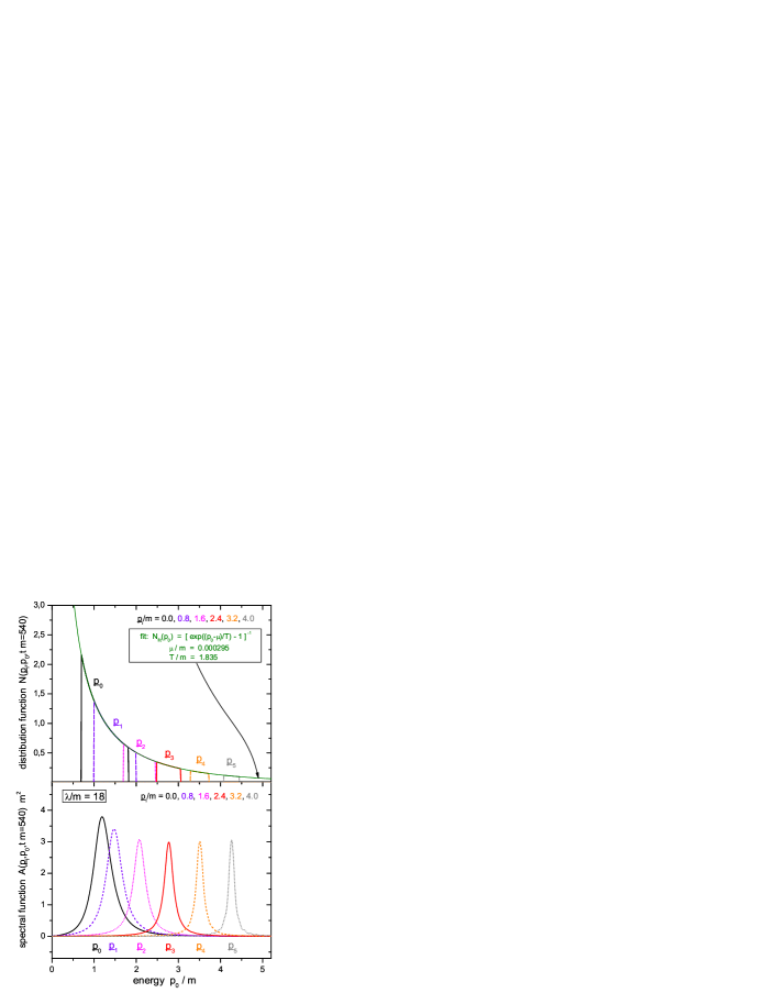
In Fig. 10 (lower part) we present the spectral function for the initial distribution D2 at late times for various momentum modes 0.0, 0.8, 1.6, 2.4, 3.2, 4.0 as a function of the energy . We note, that for all other initial distributions – with equal energy density – the spectral function looks very similar at this time since the systems proceed to the same stationary state (cf. Section IV.3). We recognize that the spectral function is quite broad, especially for the low momentum modes, while for the higher momentum modes its width is slightly lower.
The distribution function as extracted from (31) is displayed in Fig. 10 (upper part) for the same momentum modes as a function of the energy . We find that for all momentum modes can be fitted by a single Bose function with temperature . Thus the distribution function emerging from the Kadanoff-Baym time evolution for approaches a Bose function in the energy that is independent of the momentum as demanded by the equilibrium form (33).
Fig. 10 (upper part) demonstrates, furthermore, that the KMS-condition is fulfilled not only for on-shell energies, but for all . We, therefore, have obtained the full off-shell equilibrium state by integrating the Kadanoff-Baym equations in time. The comparison is achieved by selecting a certain energy band around the maximum of each momentum mode considering all energies with . In addition, the limiting stationary state is the correct equilibrium state for all energies , i.e. also away from the quasi-particle energies.
We note in closing this Subsection, that the chemical potential – used as a second fit parameter – is already close to zero for these late times as expected for the correct equilibrium state of the neutral -theory which is characterized by a vanishing chemical potential in equilibrium. This, at first sight, seems rather trivial but we will show in the next Subsection that it is a consequence of our exact treatment. In contrast, the Boltzmann equation (cf. Section V and Appendix E) in general leads to a stationary state for with a finite chemical potential. We will attribute this failure of the Boltzmann approach to the absence of particle number non-conserving processes in the quasi-particle limit (see below).
IV.4 Chemical equilibration and approach to KMS
As we have seen in the previous Subsection the chemical potential for the stationary state of the propagation at large times is close to zero in agreement with the properties of the neutral -theory. In this Subsection we will address the question of chemical equilibration in the late time evolution of the systems calculated before. In particular we are interested to examine, how the chemical potential vanishes with time for configurations initialized with finite chemical potentials at .
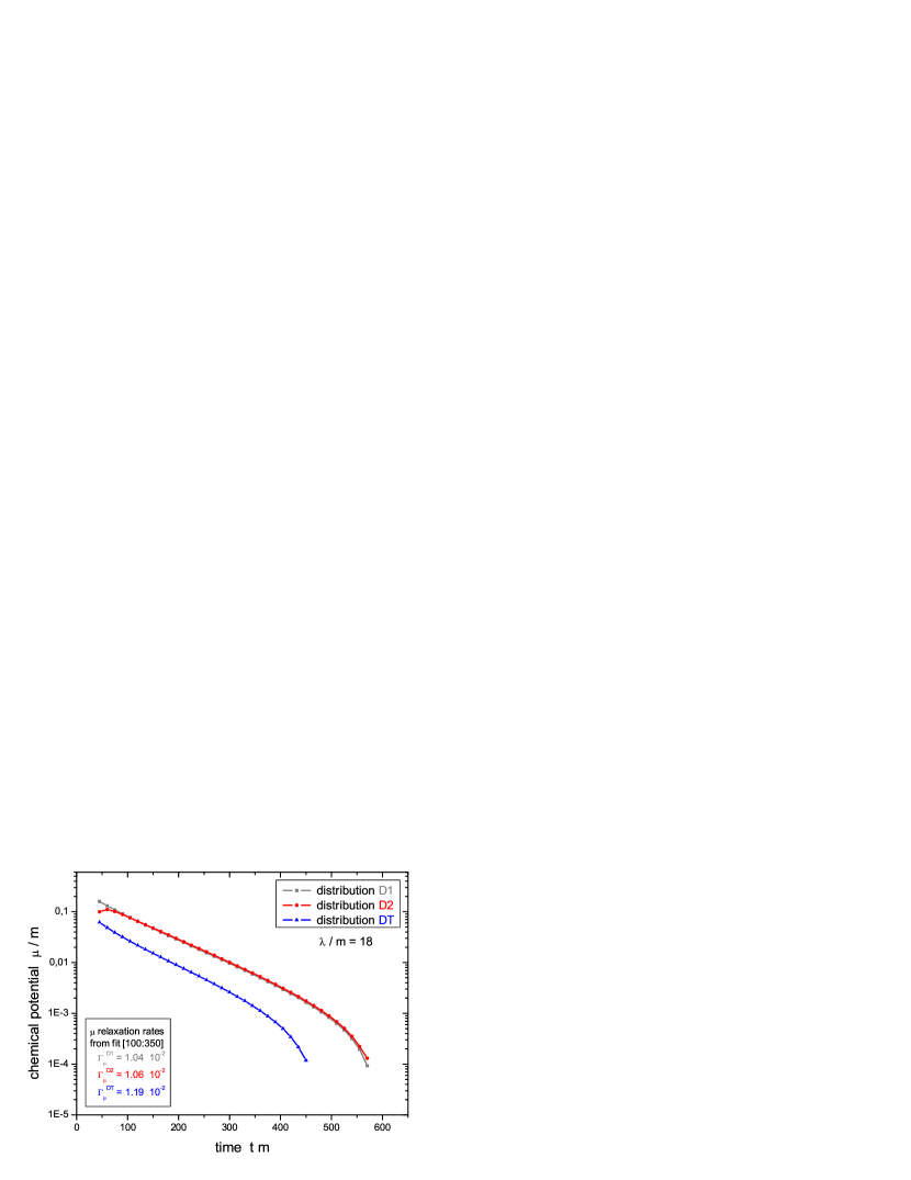
To this aim we calculate the distribution function for various system times and extract the time-dependent chemical potential by fitting a Bose function with parameters and . The time evolution of the chemical potential (as extracted from the zero momentum mode) is displayed in Fig. 11 for various initial configurations and found to decrease almost exponentially with to zero. For small times the curves do not show an exponential behaviour since here we are still in the regime of kinetic nonequilibrium. Moreover, the chemical potential relaxation rate is nearly the same for all initial configurations with the same energy density.
In order to understand the reason for this observation we calculate an estimate for this relaxation rate along the lines of Calzetta and Hu CH02 . For reasons of transparency we first provide a brief derivation for the three-loop approximation of the 2PI effective action.
Since we are interested in the properties of the system close to
equilibrium we again change to a Wigner representation for the
Kadanoff-Baym equation.
A first order gradient expansion of the Wigner transformed equation
yields the following real valued transport equation
caju1 ; caju2 ; caju3
| (34) |
Here the operator denotes the
()-dimensional representation of the general Poisson-bracket.
For the present case of spatially homogeneous systems all derivatives
with respect to the mean spatial coordinates vanish.
Thus it contains mean time and energy derivatives, only, and is given
for arbitrary functions as
| (35) |
We first concentrate on the collision term –
as given by the r.h.s. of equation (IV.4) – for
small deviations from thermal equilibrium.
In our representation the correlation self-energies
read in Wigner space
where the energy and momentum integrals extend from to
. In order to simplify the collision term we express the
Green functions (similar to (31)) by the spectral
function and a distribution function via
| (37) |
The advantage of this representation is that the spectral function
term as well as the modified
distribution function are
symmetric in the energy coordinate as can be deduced from
for the momentum symmetric () configurations considered here.
The remaining asymmetric character of the Green functions is
contained in the step-functions in energy. By this separation we
may express the integrations over the full energy space in terms
of integrations over the positive energy axis, only. Thus the
collision term – additionally integrated over momenta and positive
energies – can be written as
Here we have introduced the short-hand notation:
| (39) |
We are interested especially in the very late time evolution,
where the system is already close to equilibrium. Thus we can
evaluate the integrated collision term with further
approximations. First, we use the thermal spectral function
at the equilibrium temperature .
This spectral function is calculated separately within a
self-consistent scheme, which is explained in detail in
Appendix D.
We note in passing, that the self-consistent thermal spectral
functions (calculated numerically) are
in excellent agreement with the dynamical spectral functions in the
long time limit of the nonequilibrium Kadanoff-Baym dynamics.
Second, we adopt an equilibrium Bose
function for the symmetrical nonequilibrium distribution function
in energy, but allow for a small deviation in terms
of a small chemical potential . This chemical
potential depends on the system time as
indicated by its relaxation observed in Fig. 11,
but is assumed to be independent of energy and momentum. The near
equilibrium distribution function is thus given by
| (40) |
We now expand the integrated collision term with respect to the
small parameter around the equilibrium value
.
Since the zero-order contribution vanishes for
the collision term in equilibrium, the first non-vanishing order is
given by
with the integration weighted by the thermal spectral function
as
| (41) |
On the left-hand-side of the transport equation we neglect, furthermore, the time derivative terms of the self-energies as well as the second Poisson bracket. The only contribution then stems from the drift term , which might be extended by considering the energy derivative of the real part of the retarded self-energy.
The Green function is expressed again in terms of symmetric functions
in energy (37), where the distribution function
is given by the near equilibrium estimate
(40) with a small time-dependent deviation
.
Since the spectral function is approximated by its equilibrium form,
the time derivative of the drift term gives only a contribution from the
chemical potential. When integrating the complete drift term over
momentum and (positive) energy space – as done above for the
right-hand-side – we obtain in lowest order of the small
chemical potential
By taking also into account the energy derivative of the retarded
self-energy we gain the improved result
Combining now both half-sides of the approximated transport
equation we obtain
| (44) |
with the temperature and coupling constant dependent functions
| (45) | |||||
Thus the chemical potential decreases exponentially as
| (46) |
with the relaxation rate given by
| (47) |
The equations above provide an explanation for the observed behaviour of the relaxation of the chemical potential. At first we recognize the exponential nature (46) of the processes seen in Fig. 11. The relaxation of the chemical potential originates – as seen from (45) – from particle number non-conserving processes. This is easily recognized when considering the distribution functions assigned to incoming particles as well as the corresponding Bose enhancement factors for the outgoing ones. Ordinary particle number conserving scattering processes do not contribute. Thus it is not surprising, that a relaxation of the chemical potential is not described in the on-shell Boltzmann limit and the correct equilibrium state with vanishing chemical potential is missed (cf. Appendix E).
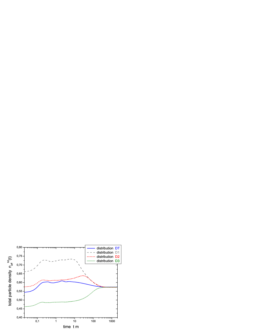
The corresponding time evolution of the total particle
number density is shown in Fig. 12.
It is obtained as the momentum space integral over the
effective distribution function, which is defined for symmetric
() configurations
by the equal-time Green functions as berges3
| (48) |
From Fig. 12 we clearly see that the particle number for the full Kadanoff-Baym equation is not constant in time, but changes due to transitions. Finally, the distributions D1, D2 and DT show an excess of particles – related to their positive chemical potential – that is reduced until the common particle number is reached in the stationary limit. In contrast, the distribution D3 (dotted line) with initially well separated maxima in momentum space has too few particles, however, during the time evolution particles are produced such that the system reaches the common equilibrium state as well.
Furthermore, we point out the importance of the spectral function entering the relaxation rate (45) via the integral measures. Since processes are responsible for the chemical equilibration, especially the shape of the spectral functions for high and low energies, i.e. above and below the three-particle threshold, is of great importance. From the formula above we also find an explanation for the fact, that all equal energy initializations – although starting with different absolute values of the chemical potential – show approximately the same relaxation rate. The spectral functions for the different initializations have already almost converged to the thermal spectral function (for the equilibrium temperature of and coupling constant ) and are therefore comparable during the late stage of the evolution. The same holds approximately for the respective distribution functions, that approach Bose distribution functions at temperature . Thus we can deduce from (45) that the relaxation rate should be approximately the same for the different initial value problems considered.
Indeed, the estimate for the chemical relaxation (47) rate works rather well quantitatively. By calculating the thermal spectral functions independently within a self-consistent scheme at equilibrium temperature for coupling constant we find (together with the distribution functions of the same temperature) – by solving the multidimensional integrations – a value of (for the drift term only) and (when including additionally the energy dependence of the retarded self-energy) for the relaxation rate. The agreement with the results of the actual calculations in Fig. 11 given by , , and , is sufficiently good.
IV.5 Dynamics close to the thermal state
In this Subsection we address the properties of systems close to thermal equilibrium. It is a widely used assumption that there exists a regime close to the thermal state, where the relaxation approximation is valid. Especially interesting are settings, where all momentum modes are in equilibrium, but only a single momentum mode is out of equilibrium and deviates from its equilibrium value by a small amount . In such a case should decrease exponentially in time. The corresponding rate can be calculated in the usual quasi-particle approximation (i.e. starting from the standard Boltzmann equation) and is given by the on-shell width of the particle as determined from the imaginary part of the retarded self-energy at the on-shell energy (with respect to the momentum ) as .
In order to study the relaxation behaviour within the full Kadanoff-Baym theory we generate a corresponding initial state by the following procedure: We first start with a general nonequilibrium distribution at and let it evolve in time. After a sufficiently long time period all momentum modes of the system get close to equilibrium. We then excite only a single momentum mode at a specific time by multiplying the equal-time Green-functions and at with a factor close to 1. As a result the corresponding effective occupation number (48) differs slightly from its equilibrium value by .
For this deviation indeed vanishes exponentially according to the full Kadanoff-Baym equations as shown in Fig. 13 for the zero momentum mode of the distribution function.
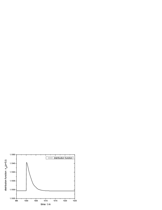
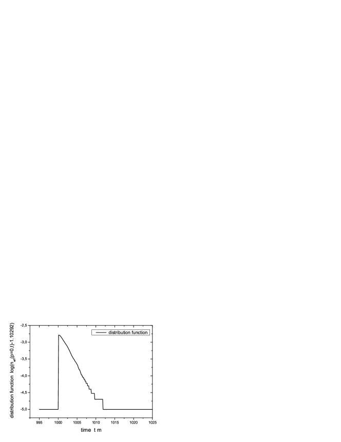
For the specific case shown in Fig. 13 the equilibrium state has been generated by starting with the initial distribution DT for a coupling constant = 18. At the time both Green-functions have been changed simultaneously by only in order to avoid large disturbances of the system. From the exponential decrease of the deviation one can directly extract the relaxation rate.
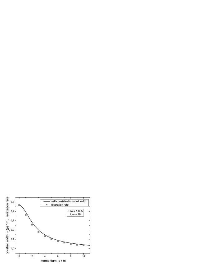
This extraction has been done for several momentum modes which leads to the numbers displayed in Fig. 14 by the full squares. In this plot, furthermore, the extracted relaxation rates are compared to the on-shell width of the particles as indicated by the line. The latter values have been obtained within an independent finite temperature calculation involving the self-consistent spectral function (and width). The exact method is described in detail in Appendix D. We note, that – apart from the coupling constant – only the equilibrium temperature enters into the self-consistent scheme as input. It yields the on-shell energies and the self-consistent width for all momenta and energies such that the on-shell width can be determined via (27). The comparison in Fig. 14 shows a very good agreement of the results for the relaxation rate obtained from a time-dependent single mode excitation of an equilibrated system with the findings for the on-shell width calculated within the self-consistent thermal approach. Thus the strong relation between both quantities has been shown explicitly for the case of a general off-shell nonequilibrium theory.
V Full versus approximate dynamics
The Kadanoff-Baym equations studied in the previous Sections represent the full quantum field theoretical equations with the chosen topology for the self-consistent dissipative self-energy on the single-particle level. However, its numerical solution is quite involved and it is of interest to investigate, in how far approximate schemes deviate from the full calculation. Nowadays, transport models are widely used in the description of quantum system out of equilibrium (cf. Introduction). Most of these models work in the ‘quasi-particle’ picture, where all particles obey a fixed energy-momentum relation and the energy is no independent degree of freedom anymore; it is determined by the momentum and the (effective) mass of the particle. Accordingly, these particles are treated with their -function spectral shape as infinitely long living, i.e. stable objects. This assumption is rather questionable e.g. for high-energy heavy ion reactions, where the particles achieve a large width due to the frequent collisions with other particles in the high density and/or high energy regime. Furthermore, this is doubtful for particles that are unstable even in the vacuum. The question, in how far the quasi-particle approximation influences the dynamics in comparison to the full Kadanoff-Baym calculation, is of general interest dan84b ; koe1 .
We also remark that the recent studies in Refs. berges1 ; berges2 ; berges3 ; CDM02 where homogeneous systems in 1+1 dimensions for the -theory have been investigated, are rather special as the on-shell 2-to-2 elastic collisions are strictly forward. Thus an on-shell Boltzmann description will not lead to any kinetic equilibration in momentum space. This is different in 2+1 dimension as we will see below.
V.1 Derivation of the Boltzmann approximation
In the following we will give a short derivation of the Boltzmann equation starting directly from the Kadanoff-Baym dynamics in the two-time and momentum-space representation as employed within this work. This derivation is briefly reviewed since we want i) to emphasize the link of the full Kadanoff-Baym equation with its approximated version and ii) to clarify the assumptions that enter the Boltzmann equation. The conventionally employed derivation of the (equivalent) Boltzmann equation will be discussed later on.
Since the Boltzmann equation describes the time evolution of
distribution functions for quasi-particles we first consider the
quasi-particle Green-functions in two-time representation for
homogeneous systems:
| (49) | |||
For each momentum the Green functions are freely oscillating in relative time with the on-shell energy . The time-dependent quasi-particle distribution functions are given with the energy variable fixed to the on-shell energy as , where the on-shell energies might depend on time as well. Such a time variation e.g. might be due to an effective mass as generated by the (renormalized) time-dependent tadpole self-energy. In this case the on-shell energy reads
| (52) |
Vice versa we can define the quasi-particle distribution function
by means of the quasi-particle Green functions at equal times
as GL98a
Using the equations of motions for the Green functions in diagonal
time direction (106) (exploiting
the time evolution of this distribution function is given by
| (54) |
The time derivatives of the on-shell energies cancel out since the
quasi-particle Green functions obey
| (55) |
as seen from (49). Furthermore, we remark that
contributions containing the energy – as
present in the equation of motion for the Green functions
(106) – no longer show up. The time evolution of the
distribution function is entirely determined by (equal-time)
collision integrals containing (time derivatives of the) Green
functions and self-energies,
| (56) | |||||
Since we are dealing with a system of on-shell quasi-particles
within the Boltzmann approximation, the Green functions in the
collision integrals (56) are given by the respective
quasi-particle quantities of (49). Moreover, the
collisional self-energies (II.2) are obtained in accordance
with the quasi-particle approximation as
| (59) | |||||
For a free theory the distribution functions are obviously constant in time which, of course, is no longer valid for an interacting system out of equilibrium. Thus one has to specify the above expressions for the quasi-particle Green functions (49) to account for the time dependence of the distribution functions.
The actual Boltzmann approximation is defined in the limit, that
the distribution functions have to be taken always at the latest
time argument of the two-time Green function koe1 ; CGreiner .
Accordingly, for the general nonequilibrium case we introduce
the ansatz for the Green functions in the collision term,
| (60) | |||||
with the maximum time . The same ansatz is employed for the time-dependent on-shell energies which enter the representation of the quasi-particle two-time Green functions (60) with their value at , i.e. .
The collision term contains a time integration which extends from
an initial time to the current time .
All two-time
Green functions and self-energies depend on the current time
as well as on the integration time . Thus only distribution functions at the current time,
i.e. the maximum time of all appearing two-time functions, enter
the collision integrals and the evolution equation for the
distribution function becomes local in time. Since the
distribution functions are given at fixed time , they
can be taken out of the time integral. When inserting the
expressions for the self-energies and the Green functions in the
collision integrals the evolution equation for the quasi-particle
distribution function reads:
| (61) | |||
| (63) |
where we have introduced the abbreviation for the quasi-particle distribution function at current time and for the according Bose factor. Furthermore, a possible time dependence of the on-shell energies is suppressed in the above notation.
The terms in the collision term (61) for particles of momentum are ordered as they describe different types of scattering processes where, however, we always find the typical gain and loss structure. The first line in (61) corresponds to the production and annihilation of four on-shell particles (, ), where a particle of momentum is produced or destroyed simultaneous with three other particles with momenta . The second line and the forth line describe () and () processes where the quasi-particle with momentum is the single one or appears with two other particles. The relevant contribution in the Boltzmann limit is the third line which respresents () scattering processes; quasi-particles with momentum can be scattered out of their momentum cell by collisions with particles of momenta (second term) or can be produced within a reaction of on-shell particles with momenta , (first term).
The time evolution of the quasi-particle distribution is given as
an initial value problem for the function
prepared at initial time . For large system times
(compared to the initial time) the time integration over the
trigonometric function results in an energy conserving
-function.
| (64) |
Here
| (65) |
represents the energy sum
which is conserved in the limit
where the initial time is considered as fixed. In this limit
the time evolution of the distribution function amounts to
| (66) | |||||
In the energy conserving long-time limit (64) only the scattering processes are non-vanishing, because all other terms do not contribute since the energy -functions can not be fulfilled for on-shell quasi-particles. Furthermore, the system evolution is explicitly local in time because it depends only on the current configuration; there are no memory effects from the integration over past times as present in the full Kadanoff-Baym equation.
In the following we will solve the
energy conserving Boltzmann equation for on-shell particles:
We point out, that the numerical algorithm for the time integration of (V.1) is basically the same as the one employed for the solution of the Kadanoff-Baym equation (cf. Appendix A). Energy conservation can be assured by a precalculation including a shift of the lower boundary to earlier times. Even small time shifts suffice to keep the kinetic energy conserved. We note, that in contrast to the Kadanoff-Baym equation no correlation energy is generated in the Boltzmann limit.
In addition to the procedure presented above, we calculate the actual momentum-dependent on-shell energy for every momentum mode by a solution of the dispersion relation including contributions from the tadpole and the real part of the (retarded) sunset self-energy. In this way one can guarantee that at every time the particles are treated as quasi-particles with the correct energy-momentum relation.
Before presenting the actual numerical results we like to comment on the derivation of the Boltzmann equation within the conventional scheme that is different from ours. Here, at first the Kadanoff-Baym equation (in coordinate space) is transformed to the Wigner representation by Fourier transformation with respect to the relative coordinates in space and time (for -theory see Refs. danmrow ; GL98a ). The problem then is formulated in terms of energy and momentum variables together with a single system time. For non-homogeneous systems a mean spatial coordinate is necessary as well. As a next step the ‘semiclassical approximation’ is introduced, which consists of a gradient expansion of the convolution integrals in coordinate space within the Wigner transformation. For the time evolution only contributions up to first order in the gradients are kept (cf. (IV.4)). Finally, the quasi-particle assumption is introduced as follows: The Green functions appearing in the transport equation – explicitly or implicitly via the self-energies – are written in Wigner representation as a product of a distribution function and the spectral function (cf. Section IV.4). The quasi-particle assumption is then realized by employing a -like form for the spectral function which connects the energy variable to the momentum. By integrating the first order transport equation over all (positive) energies, furthermore, the Boltzmann equation for the time evolution of the on-shell distribution function (V.1) is obtained.
Inspite of the fact, that the Bolzmann equation (V.1) can be obtained in different subsequent approximation schemes, it is of basic interest, how its actual solutions compare to those from the full Kadanoff-Baym dynamics.
V.2 Boltzmann vs. Kadanoff-Baym dynamics
In the following we will compare the solutions of the Boltzmann equation with the solution of the Kadanoff-Baym theory. We start with a presentation of the nonequilibrium time evolution of two colliding particle accumulations (tsunamis) boya7 within the full Kadanoff-Baym calculation (cf. Fig. 15). Such configurations are also used for simulations in the heavy-ion physics context dan84b ; boya7 ; CGreiner ; CGreinera ; koe1 .
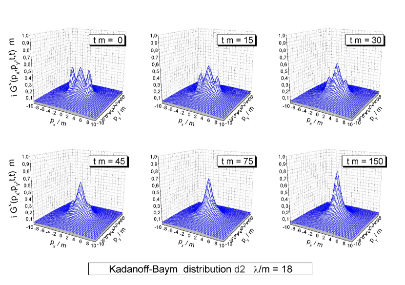
During the time evolution the bumps at finite momenta (in direction) gradually disappear, while the one close to zero momentum – which initially stems from the vacuum contribution to the Green function – is increased as seen for different snapshots at times 0, 15, 30, 45, 75, 150 in Fig. 15. The system with initially apparent collision axis slowly merges – as expected – into an isotropic final distribution in momentum space.
For the comparison between the full Kadanoff-Baym dynamics and the
Boltzmann approximation we concentrate on equilibration times. To
this aim we define a quadrupole moment for a given momentum
distribution at time as
| (68) |
which vanishes for the equilibrium state. For the Kadanoff-Baym case we use in the above expression the effective distribution function , which is determined by the equal-time Green functions (48). When constructing the distribution function by means of equal-time Green functions the energy variable has been effectively integrated out. This has the advantage that the distribution function is given independently of the actual on-shell energies. We note, that a calculation with the on-shell energies basically leads to the same results.
The relaxation of the quadrupole moment (68) has been
studied for two different initial distributions: The evolution of
distribution d2 is displayed in Fig. 15 while for
distribution d1 the position and the width of the two particle
bumps have been modified. The calculated quadrupole moment
(68) shows a nearly exponential decrease with time (see
Fig. 16) and we can extract a relaxation rate
via the relation
| (69) |
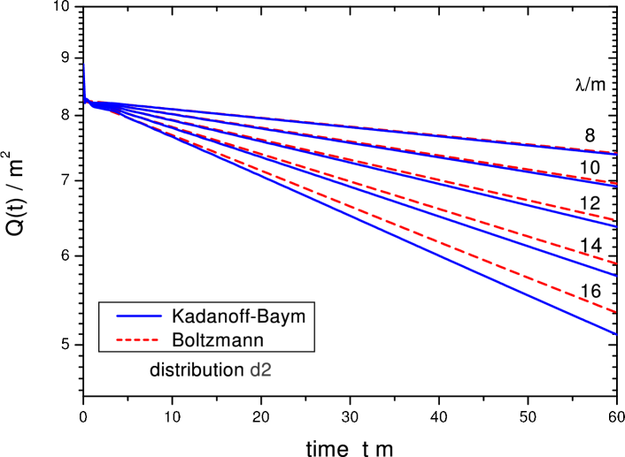
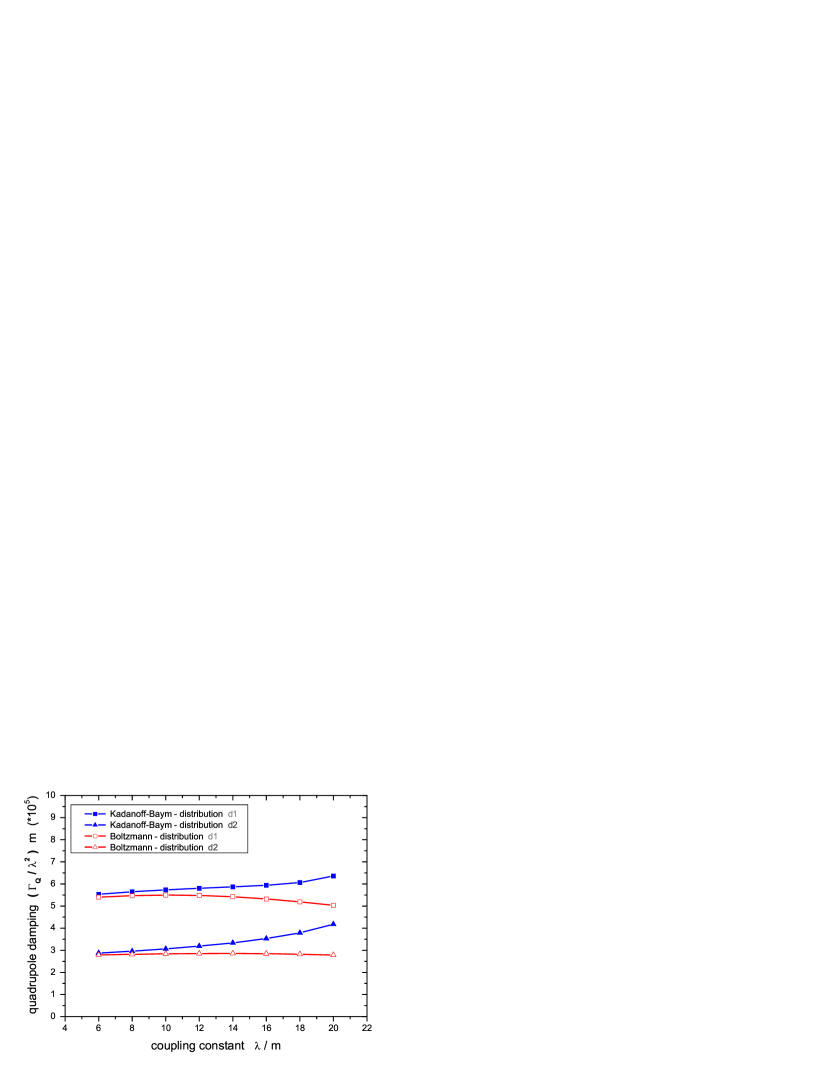
Fig. 17 shows for both initializations that the relaxation in the full quantum calculation occurs faster for large coupling constants than in the quasi-classical approximation, whereas for small couplings the equilibration times of the full and the approximate evolutions are comparable. We find that the scaled relaxation rate is nearly constant in the Boltzmann case, but increases with the coupling strength in the Kadanoff-Baym calculation (especially for the initial distribution d2).
These findings are explained as follows: Since the free Green function – as used in the Boltzmann calculation – has only support on the mass shell, only scattering processes are described in the Boltzmann limit. All other processes with a different number of incoming and outgoing particles vanish (as noted before). Within the full Kadanoff-Baym calculation this is different, since here the spectral function – determined from the self-consistent Green function (cf. Section IV.3) – aquires a finite width. Thus the Green function has support at all energies although it drops fast far off the mass shell. Especially for large coupling constants, where the spectral function is sufficiently broad, the three particle production process gives a significant contribution to the collision integral. Since the width of the spectral function increases with the interaction strength, such processes become more important in the high coupling regime. As a consequence the difference between both approaches is larger for stronger interactions as observed in Fig. 17. For small couplings in both approaches basically the usual scattering contributes and the results for the rate are quite similar.
In summarizing this Section we point out that the full solution of the Kadanoff-Baym equations does include , and off-shell collision processes which – in comparison to the Bolzmann on-shell collision limit – become important when the spectral width of the particles reaches 1/3 of the particle mass. On the other hand, the simple Boltzmann limit works surprisingly well for smaller couplings and those cases, where the spectral function is sufficiently narrow.
V.3 Estimate for the quadrupole relaxation
In this Subsection we concentrate on the quadrupole relaxation
rates observed for the full Kadanoff-Baym and the Boltzmann
approximation in order to provide a simple and intuitive
explanation for the actual values extracted in the last
Subsection. To this aim we study an idealized initial state
given by two -functions in momentum space. For symmetry
reasons they are placed on the positive and negative -axis at
. Thus the initial distribution function reads
| (70) |
where is a normalization constant. We are now interested in the time evolution of this distribution function in particular in view of the relaxation rate of the quadrupole moment. For simplicity we will explore this question employing the Boltzmann equation, since the differences between the full and the quasi-particle calculation are rather moderate.
The special form of the initial distribution
(70) has the particular advantage, that the collision term
of the Boltzmann equation can be calculated analytically at the
beginning of the evolution. We find for the time evolution of
momentum moments within the Boltzmann approximation in 2+1 space-time
dimensions:
Here can be a function of the momentum coordinates, but
is assumed to be independent of time, e.g. . Furthermore, the energy is fixed in this
quasi-particle calculation by the momentum as . For our special initial state
and for the chosen operators all contributions
of products of more than two distribution functions cancel out.
Thus the derivative of the mean value is given by
By inserting the explicit form of the initial conditions and performing the integrations over the momentum -functions we obtain for the gain term
where we take into account explicitly the different choices for
the operator . In
(V.3) we have introduced the on-shell energy
of the initial particle localization in momentum space
as well as the energies
.
Since the integration over the last two -functions in energy
yield zero, the only contribution to the integral stems from the first
term, which can be evaluated as
| (86) |
For the loss term we find (after carrying out the momentum space
integrals)
with the energy functions given as above. Due to
the appearance of in the loss term the
integration over the momentum is performed directly such
that the values of the operator are fixed. Again only the first
term of the integral gives a non-zero result and we get for the
loss term in the early time evolution
| (100) |
From (86) and
(100) we find – in agreement with the
general properties of the Boltzmann equation – that the total
particle number is conserved for our particular initial state
| (101) |
Thus the total particle number is given by
for all times .
Furthermore, for the reduction of the quadrupole moment
(calculated with the initial distribution ) we obtain
| (102) |
where the gain term does not give a contribution due to the symmetry in the momentum coordinates and .
As indicated by the numerical studies shown in the last Subsection
the quadrupole moment decreases nearly exponentially in time. Thus
assuming a decrease of the quadrupole moment of the form
we can determine the relaxation rate
as
| (103) |
with the initial value . In order to connect
this result to the initial distributions employed in our
calculations
| (104) |
we avail the corresponding representation of the -function and identify . Thus we can estimate the relaxation rate for the distribution d1 (, , , ) as and for distribution d2 (, , , ) as , respectively. In both cases an initial mass has been used. A comparison of this rather rough estimate with the results from the actual calculations shows a remarkably good agreement. When taking into account, that the effective mass slightly increases with the coupling in the full calculations, the agreement is even better.
Thus momentum relaxation in the full Kadanoff-Baym equations as well as in the Boltzmann limit can be understood in rather simple terms. Turning the argument around, we can conclude that relaxation phenomena – as described by the Kadanoff-Baym equations – do not differ very much in comparison to semi-classical limits though the full quantum off-shell propagation is invoked.
In addition, we note that the relaxation time for the quadrupole moment is one order of magnitude larger than the typical inverse damping width, which dictates the relaxation of a single mode out of equilibrium (see Subsection IV.5). Going from the equation (V.3) to equation (V.3) one notices that the Bose enhancement factors have dropped out for the further estimate of the quadrupole relaxation rate. On the other hand these factors enter crucially in the total width. For a 2+1 dimensional system these Bose factors are of special importance and increase significantly the damping width. This explains the obvious difference between the quadrupole relaxation – characterizing kinetic equilibration of a far-from-equilibrium system – and the relaxation of a single mode out of equilibrium.
VI Summary and outlook
In this work we have studied the quantum time evolution of -field theory for homogeneous systems in 2+1 space-time dimensions for far-from-equilibrium initial conditions on the basis of the Kadanoff-Baym equations. We have included the tadpole and sunset self-energies, where the tadpole contribution corresponds to a dynamical mass term and the sunset self-energy is responsible for dissipation and an equilibration of the system. Since both self-energies are ultraviolet divergent we have renormalized the theory by including proper counterterms (cf. Appendix B). The numerical solutions for different initial configurations out of equilibrium (with the same energy density) show, that the asymptotic state achieved for is the same for all initial conditions. In fact, we have shown that this asymptotic state corresponds to the exact off-shell thermal state of the system obeying the equilibrium Kubo-Martin-Schwinger (KMS) relations among the various two-point functions. Hence within these approximations the Kadanoff-Baym equations manifest irreversibility as expected from its coarse graining nature expressing the dynamics in terms solely of two-point functions.
During the equilibration we have identified three different stages which are related to i) the initial build up of correlations, ii) a kinetic thermalization and finally iii) a chemical equilibration. We find that the correlations are formed at very short times scales practically independent from the coupling strength involved. This result is in agreement with earlier studies of the nonrelativistic Kadanoff-Baym theory in the nuclear physics context koe2 . We have, furthermore, observed that during the second phase of kinetic equilibration the time evolution of the occupation numbers of states (momentum modes) may be non-monotonic; here a memory to the initial configuration is kept in the full off-shell dynamics. This is not observed in the pure kinetic Boltzmann description. In the final state, which is achieved due to chemical equilibration, we have demonstrated that the distribution functions can adequately be described by thermal Bose functions employing a temperature and chemical potential as Lagrange parameters. Since the -theory does not include an explicitly conserved quantum number, the chemical potential has to vanish in thermal equilibrium. This limit is achieved dynamically within the Kadanoff-Baym scheme by off-shell transitions that violate particle number conservation as recently conjectured in CH02 . Such processes are inhibited in the Boltzmann limit due to number-conserving on-shell scattering processes. The approach to chemical equilibrium, moreover, is found to be well described in an approximate scheme that only involves small deviations from the equilibrium state.
The spectral (‘off-shell’) distributions of the excited quantum modes have been evaluated by a Fourier transformation with respect to the time difference from the imaginary part of the retarded Green functions. For the systems investigated we have found no universal time evolution for these spectral functions, however, they differ only in the phase of kinetic nonequilibrium and rather fast approach the thermal equilibrium shapes. The width of the spectral functions increases with the coupling strength employed in the interacting theory.
Furthermore, a detailed comparison of the full quantum dynamics to approximate schemes like that of a standard kinetic (on-shell) Boltzmann equation has been performed. Our analysis shows that the consistent inclusion of the dynamical spectral function has a significant impact on relaxation phenomena. We find that far off-shell processes are also responsible for a shortening of the quadrupole relaxation rate in case of larger couplings relative to the Boltzmann limit, which is attributed again to the fact that the latter transitions are missed in the Boltzmann approximation. Nevertheless, the relaxation is rather adequately described in the Boltzmann limit for small and moderate couplings, such that the full off-shell dynamics has only a small effect on the relaxation processes in momentum space. We have shown additionally, that the relaxation rates can also approximately be determined by a simple relaxation ansatz with satisfying results.
Moreover, we have demonstrated, that the monotonous evolution within the number conserving Boltzmann limit does not approach the correct equilibrium state, but shows a finite chemical potential in the stationary limit (Appendix E). This, of course, must be considered as a shortcoming of the semi-classical on-shell approximation, which in principle could be cured by inclusion of higher order processes. Another important task in this context will be the investigation of more involved approximation schemes in terms of generalized transport equations caju1 ; caju2 ; caju3 ; Leupold ; knoll3 ; knoll2 . It is to proof, whether these gradient expansion schemes including off-shell particles yield a reliable description of the dynamics. In particular, the range of validity has to be explored depending of the actual nonequilibrium conditions. Due to the off-shell nature it is expected that the correct final state (with vanishing chemical potential) will be assumed, too.
As discussed in Appendix D, we have briefly considered the case of massless fields ( in the original Lagrangian (1)) as well. In principle, we find no qualitative difference in the dynamics of massless fields compared to the one with finite mass for moderate couplings due to the generation of an effective thermal mass by the leading tadpole diagram. However, close to a critical coupling we obtain a substantial decrease of the pole mass for the zero momentum mode, which is accompanied by a large increase of the width (cf. Fig. 24). Simultaneously the occupation number of the lowest mode changes drastically while the occupation of the higher momentum modes remain about the same. We address this effect as due to the onset of Bose condensation, where our successive iteration scheme breaks down. We note that in the present approach the system has to stay in a symmetric phase which dynamically might no longer be preferred. Thus a future investigation including non-vanishing field expectation values Peter2 will be necessary to clarify the properties of this phase transition.
Appendix A Numerical implementation
For the solution of the Kadanoff-Baym equations we have developed
a computer program which differs in several points from the
approach presented in Refs. berges1 ; berges2 . Instead of solving
the second order differential equation (II.2) we
generate a set of first order differential equations for the Green
functions in the Heisenberg picture,
| (105) | |||||
with the canonical field momentum . The first index or is always related to the
first space-time argument. Exploiting the time-reflection symmetry
of the Green functions some of the differential equations are
redundant. The required equations of motion are given as
| (106) | |||||
where is the mean time variable. Thus we
explicitly consider the propagation in the time diagonal direction
as in Ref. koe1 . In the equations of motion (106) the
current (renormalized) effective energy including the time
dependent tadpole contribution enters
| (107) |
The evolution in the direction has not be taken into account
for and since the Green
functions beyond the time diagonal () are determined
via the time reflection symmetry
from the known values for the
lower time triangle in both cases. Since there is no time
reflection symmetry for the functions, they have to
be calculated (and stored) in the whole , range.
However, we can ignore the evolution of since it is
obtained by the relation . The correlation
integrals in (106) are given by
| (109) | |||||
In (106) and (A) one can replace such that the set of equations is closed in the Green functions , and .
The disadvantage, to integrate more Green functions in time in this first-order scheme, is compensated by its good accuracy. As mentioned before, we especially take into account the propagation along the time diagonal which leads to an improved numerical precision. The set of differential equations (106) is solved by means of a 4th order Runge-Kutta algorithm. For the calculation of the self-energies we apply a Fourier-method similar to that used in Ref. dan84b ; koe1 . The self-energies (II.2), furthermore, are calculated in coordinate space where they are products of coordinate-space Green functions (that are available by Fourier transformation) and finally transformed to momentum space.
Appendix B Renormalization of -theory in 2+1 dimensions
In 2+1 space-time dimensions both self-energies (cf. Fig. (2)) incorporated in the present case are ultraviolet divergent. Since we consider particles with a finite mass no problems arise from the infrared momentum regime. The ultraviolet regime, however, has to be treated explicitly.
For the renormalization of the divergences we only assume that the
time-dependent nonequilibrium distribution functions are
decreasing for large momenta comparable to the equilibrium
distribution functions, i.e exponentially. Thus we can apply the
conventional finite temperature renormalization scheme. By
separating the real-time (equilibrium) Green functions into vacuum
() and thermal parts it becomes apparent, that only the pure
vacuum contributions of the self-energies are divergent. For the
linear divergent tadpole diagram we introduce a mass counterterm
(at the renormalized mass ) as
| (110) |
that cancels the contribution from the momentum integration of the vacuum part of the Green function.
In case of the sunset diagram only the logarithmically divergent
pure vacuum part requires a renormalization, while it remains
finite as long as at least one temperature line is involved.
Contrary to the case of 3+1 dimensions it is not necessary to
employ the involved techniques developed for the renormalization
of self-consistent theories (in equilibrium) in Refs.
knollren1 ; knollren2 . Since the divergence only appears (in
energy-momentum space) in the real part of the Feynman self-energy
at (and equivalently in the real part of the
retarded/advanced self-energies ), it can be
absorbed by another mass counterterm
at given 4-momentum and renormalized mass .
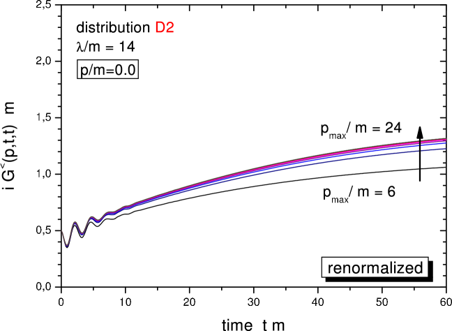
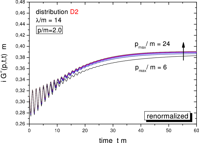
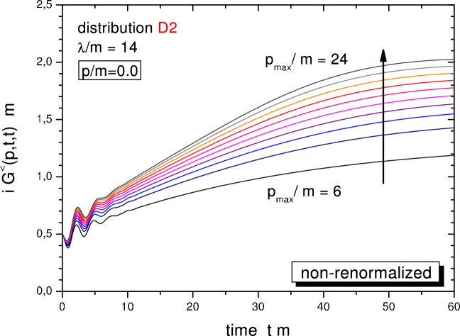
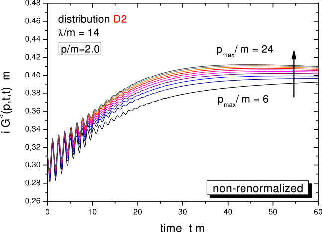
In summary, we replace the non-renormalized mass contained in the original Lagrangian (1) by with the mass counterterms given by (110) and (B). Thus the divergent part of both diagrams is subtracted. The finite part is fixed such that for the vacuum case both renormalized self-energies vanish at the renormalized mass .
In Figs. 18 and 19 we demonstrate the applicability of the renormalization prescription. To this aim we display two momentum modes = 0.0 (upper plots) and = 2.0 (lower plots) of the equal-time Green function for various momentum cut-offs 6, 8, 10, 12, 14, 16, 18, 20, 22, 24 with (cf. Fig. 18) and without (cf. Fig.19) renormalization of the sunset self-energy. For both cases the renormalization of the tadpole diagram has been used. We mention, that a non-renormalization of the tadpole self-energy has even more drastic consequences in accordance with the linear degree of divergence. For the non-renormalized calculations – with respect to the sunset diagram – we observe that both momentum modes do not converge with increasing momentum space cut-off. In fact, all lines tend to infinity when the maximum momentum is enlarged (since the gridsize of the momentum grid is kept constant). Although the divergence (as a function of the momentum cut-off) is rather weak – in accordance with the logarithmic divergence of the sunset self-energy in 2+1 space-time dimensions – a proper ultraviolet limit is not obtained.
This problem is cured by the sunset mass counterterm (B) as seen from Fig. 18. For the momentum mode the calculations converge to a limiting curve with increasing momentum cut-off. Even for the more selective case of the mode of the equal-time Green function the convergence is established. We point out that this limit is obtained for the unequal-time Green functions as well (not shown here explicitly). In fact, it turns out that the equal-time functions provide the most crucial test for the applicability of the renormalization prescription, since the divergent behaviour appears to be less pronounced for the propagation along a single time direction or . Thus we can conclude, that the renormalization scheme introduced above, i.e. including mass counterterms for the divergent tadpole and sunset self-energies, leads to ultraviolet stable results.
Appendix C General initial conditions
In Section III we briefly have described
our choice for the initial conditions for the full dynamical equations;
i.e. we have taken some particular
initial momentum distribution of interest, ,
which is then inserted in the standard quasi-particle expressions
(compare (49)):
| (112) | |||
We note that for the energy in the above expression we have taken the on-shell energy with the bare mass. This straightforward procedure, though, is not the most general form for initial conditions within the standard Kadanoff-Baym scheme. In principle, as we will outline below, there exist four independent real valued numbers for characterizing the most general initial condition instead of the two distributions and ) in (112).
To this aim we first remark that the formal solution of the
Kadanoff-Baym equations (II.1),
including all boundary conditions at the initial
time , can be cast in the form GL98a
This relation is sometimes denoted as a generalized fluctuation-dissipation theorem in the literature BB72 ; dan84a ; Ch85 ; GL98a . and represent the self-consistently dressed retarded and advanced propagator, respectively, within the real-time formalism (13, 14). Since the Kadanoff-Baym equations are second order differential equations in time for both time arguments in case of a relativistic bosonic theory, (C) obviously has to contain four independent initial real valued quantities. It is straightforward to show that and are real valued, whereas and are related to each other by complex conjugation; hence we get two further real quantities for the initial conditions. Furthermore, due to the equal-time commutation relations, one first notes that i) , and ii) . Hence, for a real relativistic field theory for scalar bosons all the various Green functions for equal times at momentum are directly related to those at momentum . In total, this proves that apart from the two distributions and there exist two further independent quantities for the initial Green functions (112). One is allowed, for example, to freely choose the real and imaginary part of instead of those stated in (112). In more physical terms, the four initial conditions correspond to the amplitudes and the phases of the two momentum modes and . In this respect the ansatz in (112) represents a statistically averaged distribution for the phases.
Inspecting further the formal solution (C), one notices that all the various terms containing the four initial conditions and contributing to are damped by the retarded and advanced propagator for times and thus will die out on a timescale of the inverse damping width (27). Correspondingly, this is also the timescale of dephasing and decoherence of the initial modes if particular phases would have been chosen initially. As an example, some moderate initial oscillations in the equal-time Green function can be seen in Fig. 4 and in Fig. 18. The modes need ‘some time’ to acquire their characteristic spectral dressing and collective phase correlations, before the further (and rather smooth) dynamics proceeds. This time is indeed roughly the inverse damping width for the various modes.
The destruction of initial (phase) correlations resembles the old conjecture of Bogolyubov Bo46 that the initial conditions do vanish after some finite time and do not show up any further in the subsequent dynamics of the system.
As a final remark we note, that one can principally also take care of higher order initial correlations within the dynamical prescription, which are not incorporated in (C) and thus in the standard Kadanoff-Baym equations Fu71 ; Ha75 ; dan84a ; He90 . We recall that the standard real-time prescription stems from a perturbative Wick-type expansion, which is valid for a special initial density operator of single-particle (Gaussian) type. The Kadanoff-Baym equations then correspond to self-consistent and resummed Dyson-Schwinger equations in real-time for a given set of skeleton-type diagrams. On the other hand, there might (or should) exist initial correlations beyond the single-particle mean-field (or Gaussian) level. As we have discussed in section IV.1, some particular higher order correlations – in this case due to the quantal collisions – will be generated dynamically during the course of the evolution. Hence, in principle, such correlations should also be taken care of in the beginning of the evolution. This is not a simple task, though: These non-trivial correlations lead to non-zero expectation values of normal-ordered operators, which can be taken care of by defining new types of contractions, which couple the time evolution of the system also to those higher order correlations. For details of such a procedure we refer the interested reader to Refs. Fu71 ; Ha75 ; dan84a ; He90 . Again one is reminded of the conjecture of Bogolyubov Bo46 that also such higher order initial correlations should die out after some finite time.
Appendix D Self-consistent spectral functions at finite temperature
Whenever dealing with strongly interacting systems the single-particle spectral function is of great importance. In particular for systems at high temperature and/or high densities the spectral functions may exhibit a large width connected to a possibly complicated structure rather than showing a -function shape as in the case of on-shell quasi-particles.
For systems in equilibrium there are two standard approaches for calculating the spectral function: i) within the imaginary time formalism (ITF) by summation over discrete Matsubara frequencies, ii) within the real-time formalism (RTF), where the energy is considered as a real and continuous variable. One great advantage of the approach ii) lies in the fact that it can be easily connected to the nonequilibrium situation. Therefore, we will use for our further developments the real-time formalism (RTF) as familiar from nonequilibrium calculations lands . We recall that the perturbative calculation of the sunset graph has been given in various works Par92 ; Je95 ; EH95 ; NMH03 . Very recently a first self-consistent treatment of the -theory in 3+1 dimensions up to this order has been presented in knollren2 .
In this Appendix we present a method for the calculation of
self-consistent spectral functions, which i) treats different order
contributions in the number of loops of the self-energy on the same
footing and ii) incorporates the finite width due to the imaginary
part of the self-energy.
Thus the actual spectral function reenters the calculation and
is iterated until self-consistency is reached.
Our iteration scheme is divided into the following steps:
1) The Green functions , are specified in energy-momentum
space .
In the initial step this can be done by assuming free Green
functions (i.e. with -function like spectral functions) at
the desired equilibrium temperature .
2) We change to the mixed representation by Fourier transformation
with respect to and calculate the Green functions , as a
function of momentum and relative time .
Since we are interested in a (static) equilibrium situation, there is no
dependence on a mean time variable.
In case of the initial on-shell Green functions the mixed
representation () is obtained analytically
(49).
3) The collisional self-energies
are calculated in the mixed representation with the Green-functions
via (II.2).
Additional remark: step 3) can be performed in several ways depending
on the explicit structure of the self-energy diagrams.
For the case of the sunset diagram in -theory we utilize
another Fourier-method. Here the self-energies are first evaluated
as a function of relative spatial (and time) coordinates,
since the sunset self-energy is (in coordinate space) simply a product
of coordinate space Green-functions that are available by
Fourier transformation with respect to the momentum.
In the final step these self-energies are transformed by a spatial
Fourier transformation back into the desired mixed representation.
4) From the collisional self-energies
we determine the retarded self-energy as
| (116) |
Thus the retarded self-energy is calculated in the mixed
representation by explicit introduction of a step-function
in relative time.
As we will discuss below this is the main advantage of our scheme
because it guarantees analyticity and thus the normalization of the
self-consistent spectral function.
5) The retarded self-energy is Fourier transformed back into
energy-momentum space and separated into its
real part and its imaginary part,
which is related to the width as
.
6) Calculating, furthermore, the purely real tadpole self-energy
the spectral function is given as
| (117) |
Here besides the initial physical mass the mass counterterms
enter, that have to
be calculated independently (see Appendix B).
The expression (117) for the spectral function is valid
in general within a first order gradient expansion of the transport
equation and is exact in equilibrium caju1 .
It is obtained as
from the Green function that solves the retarded
Dyson-Schwinger equation (15).
7) Now we can determine the Wightman functions ,
in the next iteration step in energy-momentum space by the relations
| (118) |
The separation of the Wightman functions into distribution functions
and spectral function is always possible and well-known from
the derivation of transport equations caju1 .
We recall that in thermal equilibrium the distribution function
only depends on the energy variable and is independent of
the momenta .
It is given – for the scalar theory – by the Bose distribution
| (119) |
at equilibrium temperature .
The method is not restricted to finite temperature, but can be easily
extended to finite densities.
The presence of conserved quantities, as given for a charged complex
scalar theory in the most simple case, can be accounted for by
inclusion of a corresponding chemical potential in the
Bose distribution function.
In thermal equilibrium the Wightman functions are connected by the
Kubo-Martin-Schwinger (KMS) periodicity condition
| (120) |
as inherent in the relations (118). The same holds for the collisional self-energies at finite temperature. Thus the calculations take slightly less effort than implied above.
By calculating the new Green functions in 7) we have closed the iteration loop. The iteration procedure is reentered at step 2), where the new Green functions are transformed to relative time space in order to calculate the corresponding new collisional self-energies. The alternating calculation of the Green function and of the spectral function is performed until self-consistency is reached.
The scheme proposed above has one central advantage in comparison to the related approach given in lehr . In that case an iteration loop between the Green function and the spectral function or – to be more precise – the width is used as well. The width is determined from the imaginary part of the collisional self-energies directly in energy-momentum space and inserted into the equation for the spectral function. The real part, however, is either neglected or calculated by a dispersion relation in energy. The improvement of our method lies in using the mixed representation: Since the retarded self-energy is calculated in -space with an explicit -function in relative time, analyticity is imposed automatically, i.e. the real part and the imaginary part of the retarded self-energy in energy-momentum space are connected by a dispersion relation. Furthermore, the spectral function is normalized accordingly. This is not the case for some schemes that obtain the real part and the imaginary part of the retarded self-energy by different methods. Here problems with the normalization of the spectral function and analyticity may arise. Lateron we will illustrate this point in detail.
Within that context we also note that phenomenological models frequently use form factors, i.e. non-local vertices, to cure renormalization problems. Such form factors typically have poles in the complex energy plane. Using the form factors for the calculation of real and imaginary part of a self-energy therefore messes up the analyticity properties and in general destroys the normalization of the spectral function. A proper way out is indeed the calculation of only the imaginary part of the retarded self-energy from the corresponding loop expressions including form factors. The real part is calculated afterwards from a dispersion relation to insure the correct analyticity properties. Within our -theory renormalization is a well-defined concept. Hence in our case there is no need to resort to form factors. Therefore, we can use the computationally less expensive method discussed above for the iterative calculation of the self-energies and the two-point functions.
A further advantage lies in the fact that our method, especially in combination with the Fourier-prescription for the momentum integrals, is computationally fast in comparison to standard procedures of calculating multidimensional momentum integrals. Furthermore, due to the spherical symmetry of the equilibrium state it can be performed very efficiently. Moreover, it is easily applied to all temperatures and chemical potentials, i.e. as long as the distribution function is specified.
Our scheme is appropriate for simple self-energies, as for example the sunset diagram. Basically it is applicable also for more complex diagrams since it always reduces the number of necessary integrations. The whole procedure profits from the fact that the appearing convolution integrals in momentum and energy correspond to ordinary products of coordinate-space functions. Thus the required integrations to obtain the self-energy can be reduced considerably. In case of the sunset diagram, that has only two external points (given by the coordinates of the self-energy) but no internal points, integrations can be avoided completely besides the Fourier transformation itself. For more complicated diagrams one has to integrate over the space-time coordinates of all internal points. Nevertheless, at least the contributions from the external points can be handled in a multiplicative manner rather than performing time consuming energy-momentum integrations.
Our approach of using a mixed representation of momentum and relative time (instead of the energy) is related to a method used within the imaginary time formalism (ITF). In this case a mixed representation is established as well, which is known as the Saclay-method sac1 ; sac2 . The representation is obtained by transforming from discrete and imaginary energy variables – the Matsubara frequencies (for bosons) – towards an imaginary time variable . Due to the discrete structure of the temperature dependent Matsubara frequencies the imaginary time variable is restricted by the temperature as . In contrast, in the real-time formalism (RTF) the relative time variable is unbounded in accordance with the continous energy variable . The energy integrations of the RTF correspond in the ITF to summations over the infinite number of discrete Matsubara frequencies. In case of perturbative calculations there exist comfortable expressions for the latter series which makes the calculation easier. In a self-consistent calculation the finite temperature Green functions assume a complicated structure rather than the simple on-shell form and a numerical evaluation is necessary. This is of course possible, but intricate, since the very high Matsubara-frequencies give still a considerable contribution to the series. Thus it is necessary to include all these large modes even if the retarded self-energies are rather small at high frequencies. In order to reduce the large computing time one might calculate the retarded self-energy only up to a certain Matsubara frequency ignoring the small retarded self-energy for all higher modes. For the higher modes the Green-function of the next iteration step is determined by inclusion of the frequency and momentum independent – and thus for large frequencies non-vanishing – tadpole self-energy, only. As we have tested, this prescription seems to lead to a sufficient accuracy with a reduced computational time.
When discussing the range of applicability of our method one should note as well, that it is mainly suited for field theories that are void of complicated renormalization prescriptions. In our case of -theory in 2+1 space-time dimensions the renormalization can be done by simple mass counterterms since only the pure vacuum contributions of both self-energies diverge. This mass renormalization scheme can be easily included in the iteration procedure as seen by the representation for the spectral function (117). In cases of diverging diagrams, that contain temperature dependent parts, the renormalization procedure is much more involved knollren1 ; knollren2 . In such situations our method might be complicated significantly.
In the following we show the actual results calculated within the self-consistent scheme described above. The tadpole self-energy as well as the retarded sunset self-energy are included self-consistently using the renormalization prescription of Appendix B. In Fig. 20 the width is displayed as a function of the energy for four different momentum modes 0, 2, 4, 6 for a temperature of and a coupling constant of . This configuration corresponds to the thermalized state obtained by the time evolution of the polar symmetric initial momentum distributions D1, D2, D3 and DT in Section III. For comparison we present, furthermore, the width as obtained by a perturbative calculation (as indicated by the dashed lines) for the same momentum modes, and with the same external parameters and . The results have been obtained with the (self-consistent) effective mass on the tadpole level, i.e. by the iterative solution of the tadpole gap equation. This is in the spirit of Wang and Heinz EH95 who firstly determined the effective mass in lowest order (also in a self-consistent way) and inserted this mass in the following into the expressions for the width calculated within the next order. We see from Fig. 20 that the perturbative width shows a similar (two maxima) shape for all momentum modes (for the given case of ). It is characterized by an increase towards a maximum around the on-shell energy and falling off beyond. This behaviour stems from the processes in the self-energies as indicated for the highest momentum mode by the thin line. Particles can be scattered by other particles – present in the system at finite temperature – such that they achieve the shown (collisional) damping width. This collision contribution vanishes for a system at temperature . Furthermore, particles with sufficient energy can decay into three other particles. Above the threshold of these processes lead to an increase of the width (as marked for the highest momentum mode by the second thin line). Finally, the width decreases for larger energies and assumes a momentum independent constant value in the high energy limit. This behaviour is in contrast to the case of 3+1 dimensions, where the width shows a monotonous increase for very high energies.
In comparison, the width calculated within the self-consistent scheme shows a similar two maximum shape. Here, both processes are incorporated although they cannot be separated easily due to the self-consistent iteration. Apparently, the sharp structures present in the perturbative calculation have been washed out considerably. The kink structures resulting from threshold effects slightly disappear since the (broad) spectral function reenters the evaluation in this iteration scheme. Furthermore, also the position of the first maximum can be moved, as seen especially for the low momentum modes. This is an effect of the self-consistent spectral function that accounts also for mass shifts caused by the tadpole self-energy and the real part of the retarded sunset self-energy. Overall, Fig. 20 shows that the width in the self-consistent calculation can be significantly larger than in the corresponding perturbative estimate.
In Fig. 21 we present the corresponding spectral functions for the system at temperature and coupling constant . The spectral functions are displayed as a function of the energy for the same four momentum modes of 0, 2, 4, 6. We observe that the larger width of the full self-consistent calculation (solid lines) in comparison to the perturbative result (dashed lines in Fig. 21) reflects itself in a slightly broader spectral function. Furthermore, the perturbative spectral function is located at higher energies compared to the full result, in particular for the low momentum modes. This is due to the fact, that in the perturbative calculation the effective mass of the particles is fixed before evaluating the width by a solution of the tadpole gap equation. Mass modifications due to the interactions of higher order are neglected within this approximation in line with EH95 , where the spectral function is determined solely by the imaginary part of the retarded self-energy. On the other hand, the reduction of the effective mass due to the real part of the retarded sunset self-energy is included in the self-consistent approach leading to a shift of the spectral function maxima to lower on-shell energies. Moreover, the tadpole mass-shift is not fixed in that calculation but modified during the iteration process as well. In the present case the momentum and energy independent tadpole mass shift within the self-consistent second order calculation is given as in comparison to the value obtained for the first order calculation by the tadpole gap equation of . This indicates already a shift of the spectral function to lower on-shell energies although the size is small compared to the effect coming from the second order self-energy. Thus both spectral functions are getting closer again for higher momenta where the sunset mass shift is smaller.
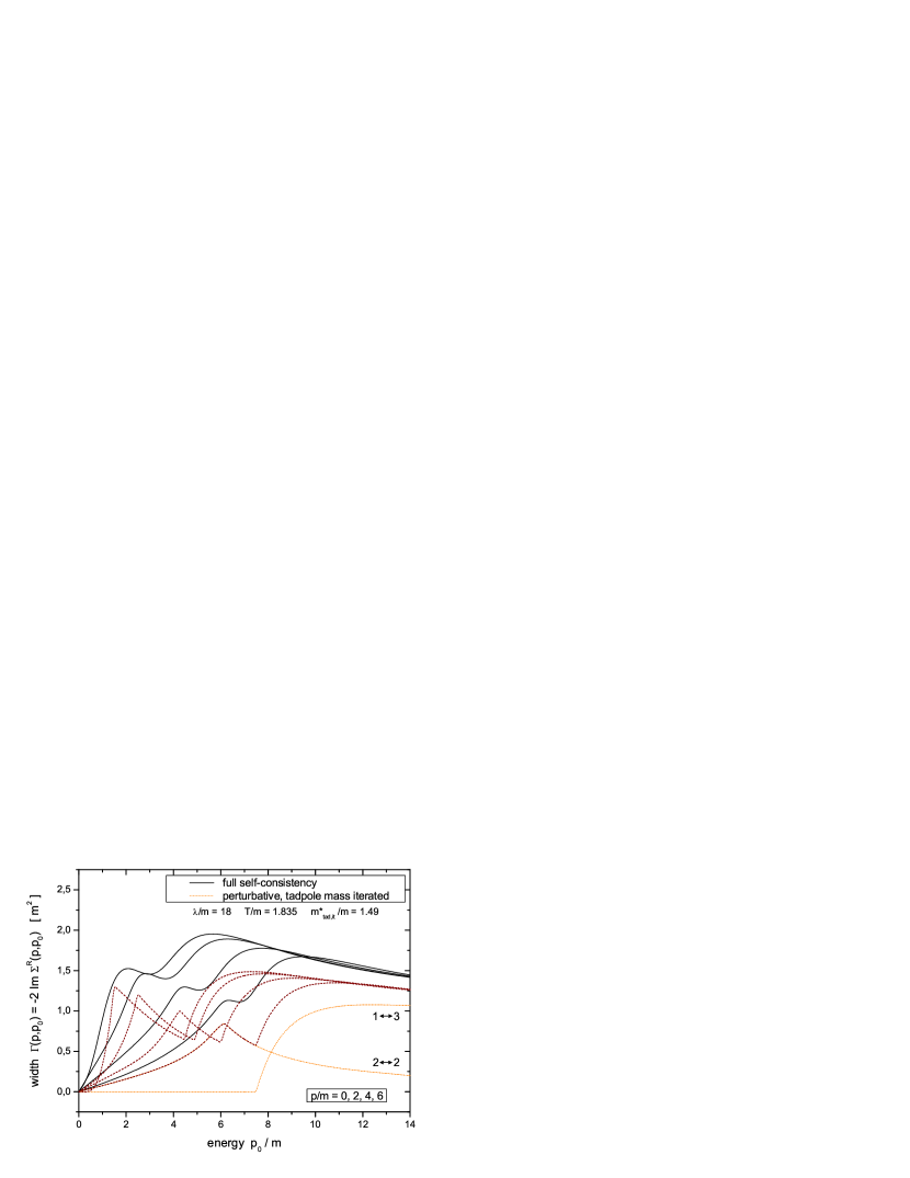
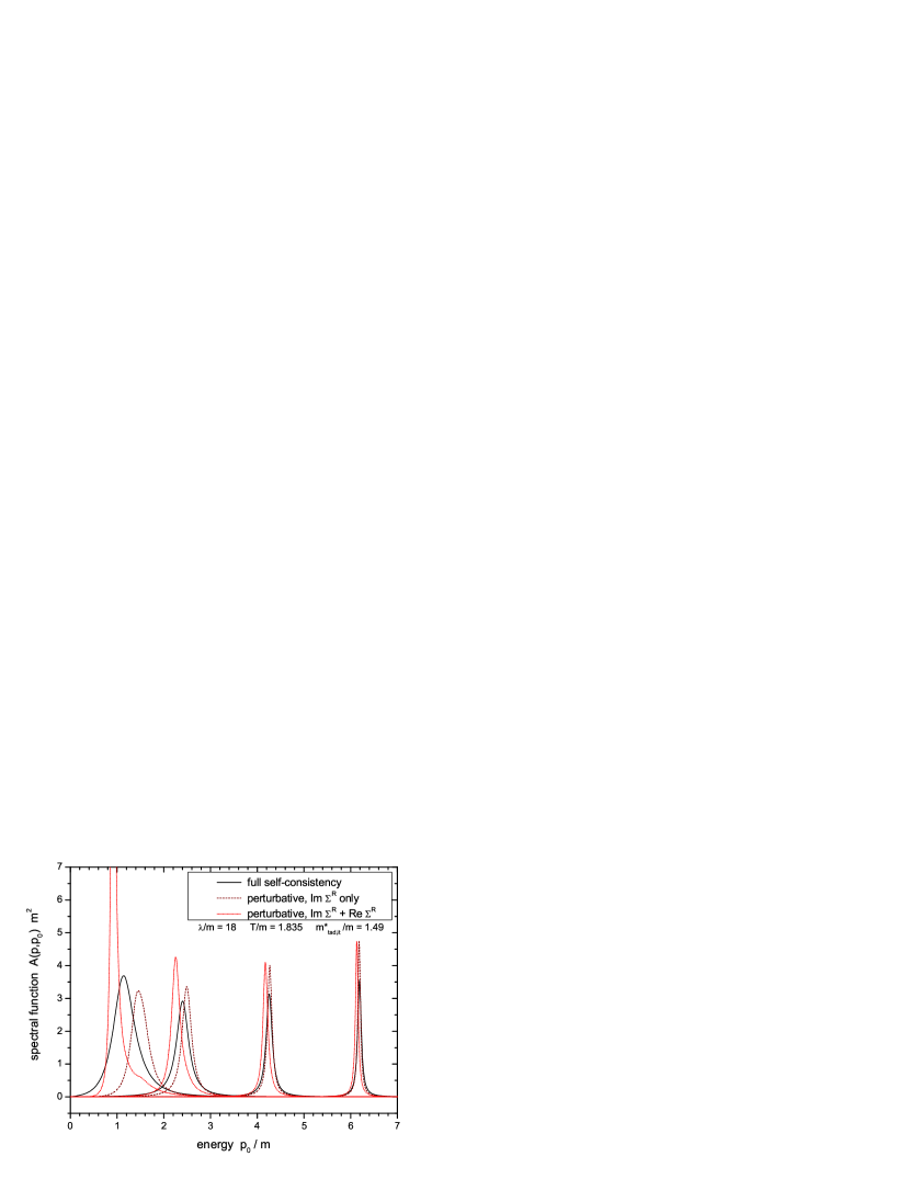
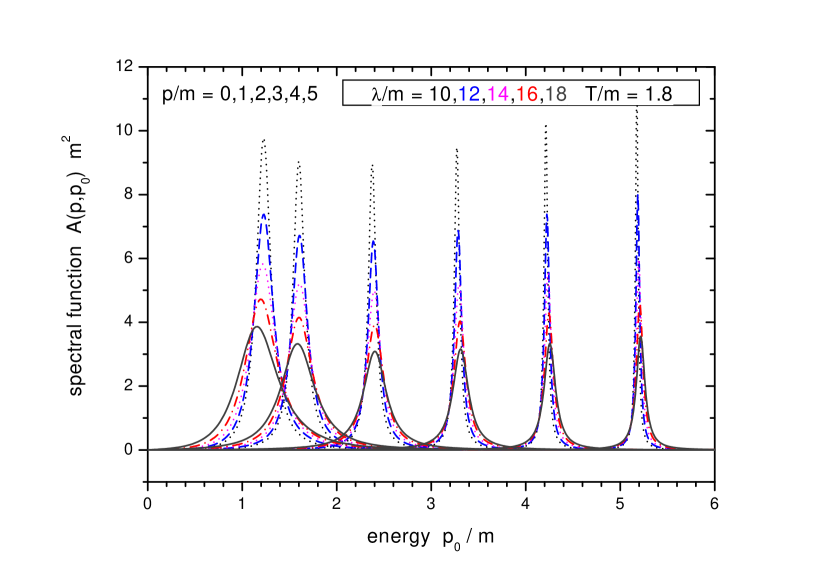
At this point we emphasize that the spectral function obtained by the self-consistent scheme obeys the normalization condition to high accuracy (26). This is not the case for a perturbative calculation where only the imaginary part of the retarded self-energy is taken into account as in EH95 . When inserting only the expression for the width into the equilibrium form of the spectral function but neglecting the real part of the retarded self-energy, the normalization condition may be violated strongly. In the present perturbative calculation the correct normalization is underestimated by for the small momentum modes. Thus these kinds of spectral functions, furthermore, strongly violate the desired analyticity properties. In order to show the importance of the real part of the retarded self-energy even on the shape of the spectral function we present in Figure 21 a calculation which takes this contribution explicitly into account. Calculating the complete retarded self-energy perturbatively with an effective mass of yields the spectral function displayed for the same momentum modes with dotted lines. We see that the shape of the spectral function is strongly affected in particular for the small momentum modes. The inclusion of the real part causes a significant shift of the spectral function downwards to lower energies. Since the width is smaller in that region (cf. Fig. 20), the spectral function assumes – especially for the low momentum modes – a much narrower shape. Nevertheless, the inclusion of the real part of the retarded self-energy leads to a proper normalization of the corresponding spectral functions. Still there is a significant disagreement between the improved perturbative (dotted line) and the self-consistent solution (solid line).
In order to illustrate the dependence on the interaction strength we show in Fig. 22 the spectral function at temperature for coupling constants . As expected, the spectral functions are significantly broader for increasing interaction strength. Again the low lying momentum modes achieve the broadest shape, respectively. Furthermore, the on-shell value is changing with , which is easily visible for the small momentum modes. Here two effects are superimposed: The upward mass shift generated by the tadpole diagram is competing with the negative shift from the retarded self-energy, which gives a significant contribution primarily in the low momentum regime. With increasing coupling strength the higher order term dominates which results in a lowering of the on-shell energies for small momenta as seen in Fig. 22. In the high momentum region – where the real part of the retarded self-energy is small – the constant tadpole mass shift dominates and leads to an increase of the effective mass with the coupling constant. This effect can already be seen for the modes 4, 5 and is even stronger for higher momenta (not displayed here).
As the final part of this Appendix we consider the case of massless scalar fields in the Lagrangian (1). The dynamics of massless quantum field theory has been extensively discussed over the last years especially for the dynamics of the soft, infrared modes which might be described by classical wave dynamics. In particular the diffusion rate of the topological charge in electroweak theory has been calculated within classical simulations Gri . The connection between classical and quantal correlation functions has then been worked out in a variety of papers Aa96 . Also it was shown recently within -theory that the classical wave dynamics is equivalent to a standard Boltzmann description for the soft modes when including the correct Bose statistics and staying in the weak coupling regime MS02 .
We see no qualitative difference in the dynamics of massless fields compared to the one with finite masses for moderate couplings. This is the case due to the generation of an effective thermal mass by the leading tadpole diagram as suggested in mrow . We note that there is a logarithmic divergence in the infrared sector for the sunset self-energy in vacuum for 2+1 dimensions (cf. (B)) and thus a sublety, which we have cured by evaluating the vacuum counterterm in our renormalization description at a very small but finite mass.
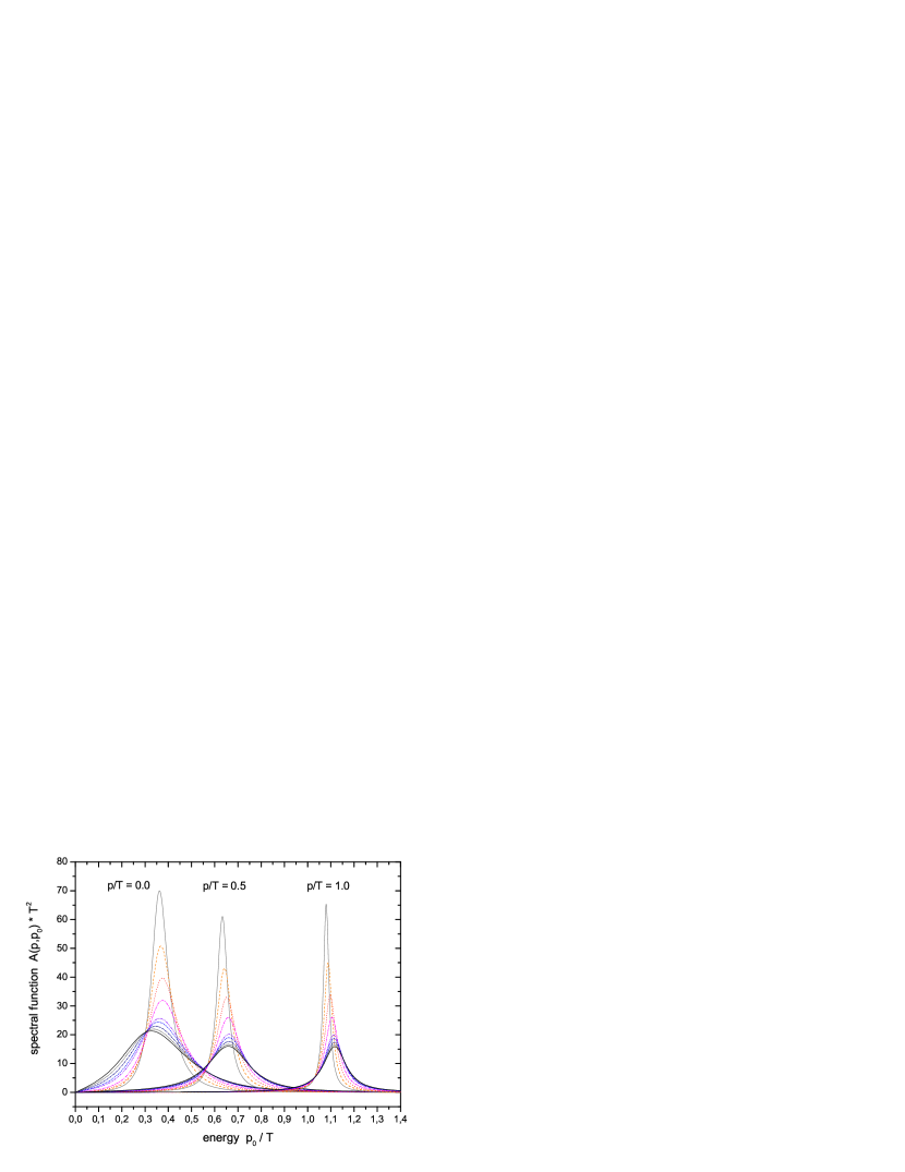
In the following we concentrate on the structure of the spectral function in dependence of the coupling strength . In Fig. 23 the spectral function of three low momentum modes 0.0, 0.5, 1.0 for various coupling constants 2, 2.5, 3, 3.5, 4, 4.1, 4.2, 4.25, 4.265 as a function of energy is displayed. Since the temperature represents the scale for the massless case, we give all quantities in units of . We find that the spectral function is shifted to larger energies with increasing and still moderate coupling strength (). However, in the strong coupling regime () especially the spectral function of the zero momentum mode moves downward again, leading to a major reduction of the effective mass. Simultaneously, the spectral width grows with the coupling constant . Thus for large couplings the on-shell width becomes comparable to the effective mass (as given by the maximum position of the zero mode spectral function).
To summarize our findings we show in Fig. 24 (upper part) the evolution of the on-shell energy of the zero momentum mode as a function of the coupling constant . The effective mass – as given by the maximum of the spectral function – increases with up to moderate couplings which is – as already discussed for the non-zero mass case – essentially an effect of the mass generation by the tadpole self-energy. For larger couplings the contribution from the retarded self-energy plays a more important role and results in a decrease of the effective mass. The reduction of the effective mass becomes rather strong for couplings indicating a significant shift of the corresponding self-consistent spectral function to smaller energies. This behaviour is accompanied by a strong increase of the on-shell width of the zero momentum mode as seen from Fig. 24 (middle part). While the width grows smoothly with the coupling constant for moderate couplings, we find a strong steepening in the high coupling regime as well. Thus the zero mode spectral function for high coupling constants becomes extremely broad with an on-shell width comparable to or even larger than its effective mass.
As seen from Fig. 24 the evolution of the self-consistent spectral function in the strong coupling regime becomes singular and critical, such that the iteration processes do not lead to a convergent result anymore for . We address this effect to the onset of Bose condensation. In order to illustrate this interpretation we show in Fig. 24 (lower part) the change of the effective occupation number (as obtained from the equal-time Green functions (48)) with the coupling for four different momentum modes 0.0, 0.5, 1.0, 1.5. Whereas the effective particle number of the higher momentum modes remain approximately constant, the occupation number of the zero momentum mode changes rapidly for indicating a preferential occupation of the condensate mode for higher couplings.
We recall that such an onset of a Bose condensation is possible for the massless relativistic theory in 2+1 space-time dimensions. Although the effective mass is not identical to zero we observe significant spectral support at low energies due to the broad spectral functions for the strongly interacting system. We note that in the present description the system has to stay in the symmetric phase, where no coherent field can develop. However, when including additionally a non-vanishing field expectation value Peter2 , the symmetry will be broken and the system might enter a new phase. A detailed investigation of the issue we delay to a future study.


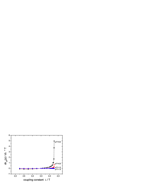
Appendix E Stationary state of the Boltzmann evolution
In Sections III and IV we have described the characteristics of equilibration within the full Kadanoff-Baym theory. In this Appendix we additionally show the nonequilibrium evolution in the Boltzmann limit and in particular work out the differences in both approaches.
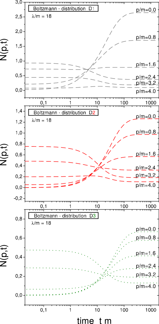
In Fig. 25 we present the time evolution of various momentum modes for the initial momentum space distributions D1, D2, D3 within the Boltzmann equation. In these calculations the effective on-shell energies are determined by including the time-dependent renormalized tadpole self-energy. The distributions D1, D2, D3 have been modified relative to our study of the Kadanoff-Baym dynamics in Section III such that they i) have the same energy density with respect to the modified total energy (where all sunset contributions are missing) and ii) are self-consistent with respect to the effective tadpole mass in order to avoid strong initial oscillations induced by a sudden change of the on-shell energies at very early times. For completeness we note, that the initial effective masses are determined by the solution of a gap equation taking into account the energy- and momentum-independent tadpole self-energy for the given initial momentum distribution.
We see from Fig. 25 that the time evolution given by the on-shell Boltzmann approximation deviates in several aspects from the Kadanoff-Baym dynamics. At first we find that in case of the Boltzmann equation the equal-energy initial distributions D1, D2 and D3 equilibrate towards different stationary states for . This can directly been read off from Fig. 25 when comparing the final occupation numbers of the various momentum modes. This behaviour is in contrast to the Kadanoff-Baym evolution where all initial distributions with the same energy reach a common stationary state (cf. Fig. 4). As pointed out in Section IV.4 this is an effect of the chemical equilibration mediated by particle number non-conserving processes, which are included in the Kadanoff-Baym dynamics since the full spectral function is taken into account. For the on-shell Boltzmann approximation, however, the particle number is strictly conserved and thus the initializations D1, D2, D3, that contain different number of particles, can not approach the same final state. Accordingly, the stationary state of the non-thermal initializations D1, D2, D3 exhibits a finite chemical potential (see below). Without explicit representation we note that the self-consistent initial configuration DT is already the thermal state of the Boltzmann equation and all momentum modes remain constant in time, whereas within the Kadanoff-Baym dynamics the ‘free’ thermal initialization DT evolves in time due to the generation of correlations (cf. Section IV.1).
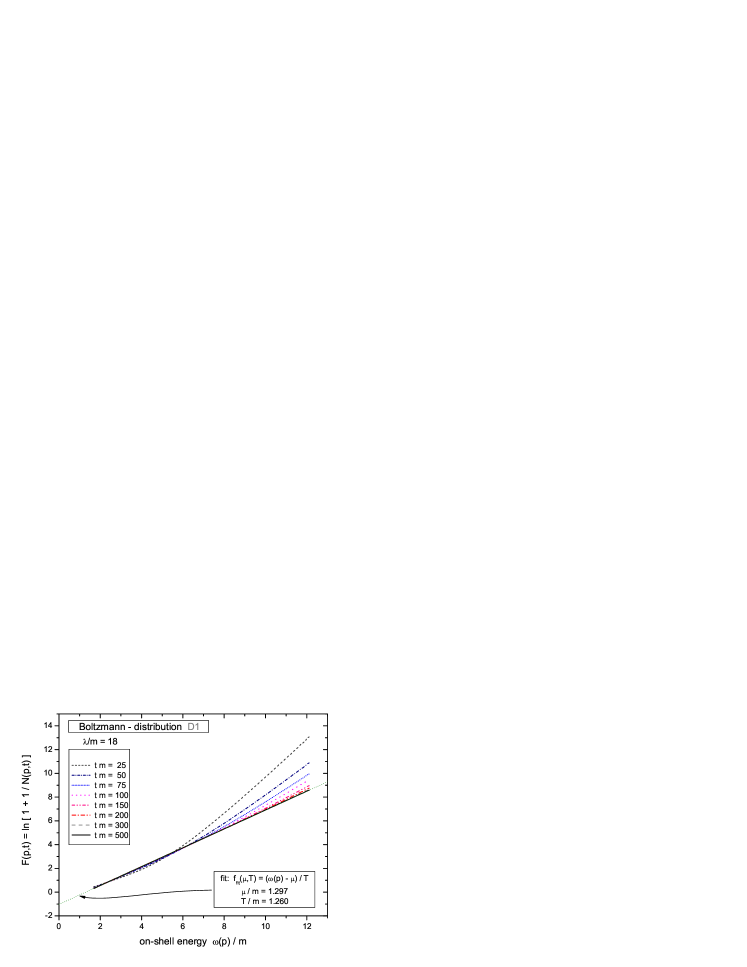
In order to demonstrate, that the time evolution on the basis of the
Boltzmann equation leads to a thermal state of quasi-particle
excitations, we show in Fig. 26 the on-shell
distribution as a function of the time-dependent on-shell
energy for
various times 25, 50, 75, 100, 150, 200, 300, 500
for the initialization D1 and coupling strength 18.
We have displayed the quantity
| (121) |
in order to obtain a straight line with slope and intersection point in case of a Bose distribution with temperature and chemical potential . We see from Fig. 26 that the distribution at early times ( = 25) is small for very low and very high momenta as reflected by the high values of the quantity in the low and high energy regime. The particle accumulation at finite momentum for initialization D1 (cf. Fig. 3 (lower part)) shows up as a small dip in the curve. In course of the time evolution these structures slowly vanish such that finally a straight line is reached (see lines for 300, 500) indicating that the stationary limit is indeed a thermal distribution (at temperature ). However, the chemical potential of the stationary distribution is non-vanishing – as recognized by the non-zero intersect of the dotted fit function – as . The initializations D2, D3 achieve different asymptotic temperatures which are given by for D2 and for D3. The chemical potential of the stationary state for these distributions is non-zero as well and has the values for D2 and for D3. We recall, that systems with large chemical potential distribute the total energy on many particles such that the final temperature is considerably lower. Thus, in general, the Boltzmann approximation does not drive the system to the proper equilibrium state of the neutral -theory, which is characterized by a vanishing chemical potential.
Furthermore, we see from Fig. 25 that in the Boltzmann limit the momentum modes evolve monotonically in time; there is no overshooting of the stationary limit as observed in the Kadanoff-Baym picture (cf. Fig. 4). Thus the non-monotonic behaviour shows up as a quantum phenomenon that is missing in the semi-classical treatment.
Acknowledgements.
The authors thank S. Leupold for various discussions throughout our investigations. This work was supported by GSI Darmstadt and DFG.References
- (1) D. H. Lyth and A. Riotto, Phys. Rept. 314 (1999) 1; A. Riotto and M. Trodden, Ann. Rev. Nucl. Part. Sci. 49 (1999) 35; M. Trodden, Rev. Mod. Phys. 71 (1999) 1463.
- (2) D. Boyanovsky, H. J. de Vega, R. Holman, and J. F. J. Salgado, Phys. Rev. D 54 (1996) 7570.
- (3) L. Kofman, A. Linde, and A. A. Starobinsky, Phys. Rev. D 56 (1997) 3258.
- (4) M. Gell-Mann and J. B. Hartle, Phys. Rev. D 47 (1993) 3345.
- (5) B. Müller, ‘The Physics of the Quark-Gluon Plasma’, Lecture Notes in Physics 225 (1985), Springer, Berlin; ‘Quark-Gluon Plasma’, ed. R. Hwa, Advanced Series on Directions in High Energy Physics, World Scientific, (1990); ‘Quark-Gluon Plasma II’, ed. R. Hwa, Advanced Series on Directions in High Energy Physics, World Scientific, (1995).
- (6) for a review see the contribution of K. Rajagopal in ‘Quark-Gluon Plasma II’ in Mul85 .
- (7) D. Boyanovsky, H. J. de Vega, and R. Holman, Phys. Rev. D 51 (1995) 734; F. Cooper, Y. Kluger, E. Mottola, and J. P. Paz, Phys. Rev. D 51 (1995) 2377.
- (8) T. S. Biro and C. Greiner, Phys. Rev. Lett. 79 (1997) 3138; Z. Xu and C. Greiner, Phys. Rev. D 62 (2000) 030612.
- (9) J. Schwinger, J. Math. Phys. 2 (1961) 407.
- (10) P. M. Bakshi and K. T. Mahanthappa, J. Math. Phys. 4 (1963) 1, 12.
- (11) L. V. Keldysh, Zh. Eks. Teor. Fiz. 47 (1964) 1515; Sov. Phys. JETP 20 (1965) 1018.
- (12) R. A. Craig, J. Math. Phys. 9 (1968) 605.
- (13) L. P. Kadanoff and G. Baym, Quantum statistical mechanics, Benjamin, New York, 1962.
- (14) D. F. DuBois in Lectures in Theoretical Physics, edited by W. E. Brittin (Gordon and Breach, NY 1967), pp 469-619.
- (15) P. Danielewicz, Ann. Phys. (N.Y.) 152 (1984) 239.
- (16) K. Chou, Z. Su, B. Hao, and L. Yu, Phys. Rept. 118 (1985) 1.
- (17) J. Rammer and H. Smith, Rev. Mod. Phys. 58 (1986) 323.
- (18) E. Calzetta and B. L. Hu, Phys. Rev. D 37 (1988) 2878.
- (19) H. Haug and A. P. Jauho, Quantum Kinetics in Transport and Optics of Semiconductors, Springer, New York, 1999.
- (20) C. Greiner and S. Leupold, Ann. Phys. 270 (1998) 328.
- (21) W. Cassing, Z. Physik A 327 (1987) 447.
- (22) W. Cassing, K. Niita, and S. J. Wang, Z. Physik A 331 (1988) 439.
- (23) W. Cassing, V. Metag, U. Mosel, and K. Niita, Phys. Rept. 188 (1990) 363.
- (24) B. Bezzerides and D. F. DuBois, Ann. Phys. 70 (1972).
- (25) P. Lipavský, V. Špička, and B. Velický, Phys. Rev. B 34 (1986) 6933.
- (26) W. Botermans and R. Malfliet, Phys. Rept. 198 (1990) 115.
- (27) S. Mrówczyński and P. Danielewicz, Nucl. Phys. B 342 (1990) 345.
- (28) V. Špička and P. Lipavský, Phys. Rev. Lett. 73 (1994) 3439; Phys. Rev. B 52 (1995) 14615.
- (29) A. Makhlin, Phys. Rev. C 52 (1995) 995; A. Makhlin and E. Surdutovich, Phys. Rev. C 58 (1998) 389.
- (30) K. Geiger, Phys. Rev. D 54 (1996) 949; Phys. Rev. D 56 (1997) 2665.
- (31) D. A. Brown and P. Danielewicz, Phys. Rev. D 58 (1998) 094003.
- (32) J. P. Blaizot and E. Iancu, Nucl. Phys. B 557 (1999) 183.
- (33) M. Imamovic-Tomasovic and A. Griffin, Phys. Rev. A (1999) 494.
- (34) Y. B. Ivanov, J. Knoll, and D. N. Voskresensky, Nucl. Phys. A 657 (1999) 413.
- (35) J. Knoll, Y. B. Ivanov, and D. N. Voskresensky, Ann. Phys. 293 (2001) 126.
- (36) F. Cooper, S. Habib, Y. Kluger, E. Mottola, J. P. Paz, and P. R. Anderson, Phys. Rev. D 50 (1994) 2848.
- (37) D. Boyanovsky, H. J. de Vega, R. Holman, D.-S. Lee, and A. Singh, Phys. Rev. D 51 (1995) 4419.
- (38) D. Boyanovsky, M. D’Attanasio, H. J. de Vega, R. Holman, and D.-S. Lee, Phys. Rev. D 52 (1995) 6805.
- (39) D. Boyanovsky, H. J. de Vega, R. Holman, S. P. Kumar, and R. Pisarski, Phys. Rev. D 57 (1998) 3653.
- (40) J. W. Negele, Rev. Mod. Phys. 54 (1982) 913.
- (41) D. Boyanovsky, I. D. Lawrie, and D.-S. Lee, Phys. Rev. D 54 (1996) 4013.
- (42) D. Boyanovsky, H. J. de Vega, R. Holman, S. P. Kumar, R. D. Pisarski, and J. Salgado, Phys. Rev. D 58 (1998) 125009.
- (43) D. Boyanovsky, H. J. de Vega, R. Holman, and M. Simionato, Phys. Rev. D 60 (1999) 065003.
- (44) E. A. Calzetta and B. L. Hu, arXiv:hep-ph/0205271.
- (45) S. Sengupta, F. C. Khanna, and S. P. Kim, arXiv:hep-ph/0301071.
- (46) A. Peter, W. Cassing, J. M. Häuser, and A. Pfitzner, Nucl. Phys. A 573 (1994) 93.
- (47) S. J. Wang, W. Zuo, and W. Cassing, Nucl. Phys. A 573 (1994) 245.
- (48) J. M. Häuser, W. Cassing, A. Peter, and M. H. Thoma, Z. Phys. A 353 (1995) 301.
- (49) A. Peter, W. Cassing, J. M. Häuser, and M. H. Thoma, Z. Phys. C 71 (1996) 515.
- (50) A. Peter, W. Cassing, J. M. Häuser, and M. H. Thoma, Z. Phys. A 358 (1997) 91.
- (51) J. M. Häuser, W. Cassing, S. Leupold, and M. H. Thoma, Ann. Phys. 265 (1998) 155.
- (52) T. Altherr and D. Seibert, Phys. Lett. B 333 (1994) 149.
- (53) C. Greiner and S. Leupold, Eur. Phys. J. C 8 (1999) 517.
- (54) P. Danielewicz, Ann. Phys. (N.Y.) 152 (1984) 305.
- (55) C. Greiner, K. Wagner, and P.-G. Reinhard, Phys. Rev. C 49 (1994) 1693.
- (56) C. Greiner, K. Wagner, and P.-G. Reinhard, ‘Finite Memory in the collision process of a fermionic system and its effect on relativistic heavy ion collisions’, Proc. of the NATO Advanced Study Institute on ‘Hot und Dense Matter’, Bodrum, Turkey, 1993, eds. W. Greiner, H. Stöcker und A. Gallmann, NATO ASI Series B, Physics, Vol. 335, plenum press (1994).
- (57) H. S. Köhler, Phys. Rev. C 51 (1995) 3232.
- (58) H. S. Köhler and K. Morawetz, Eur. Phys. J. A 4 (1999) 291; Phys. Rev. C 64 (2001) 024613.
- (59) L. Banyai, D. B. Tran Thoai, E. Reitsamer, H. Haug, D. Steinbach, M. U. Wehner, M. Wegener, T. Marschner, and W. Stoltz, Phys. Rev. Lett. 75 (1995) 2188; L. Banyai, Q. T. Vu, B. Mieck, and H. Haug, Phys. Rev. Lett. 81 (1998) 882; Q. T. Vu, H. Haug, W. A. Hügel, S. Chatterjee, and M. Wegener, Phys. Rev. Lett. 81 (2000) 3508.
- (60) A. Wackert, A. Jauho, S. Rott, A. Markus, P. Binder, and G. Döhler, Phys. Rev. Lett. 83 (1999) 836.
- (61) J. Berges and J. Cox, Phys. Lett. B 517 (2001) 369.
- (62) G. Aarts and J. Berges, Phys. Rev. D 64 (2001) 105010.
- (63) J. Berges, Nucl. Phys. A 699 (2002) 847.
- (64) F. Cooper, J. F. Dawson, and B. Mihaila, Phys. Rev. D 67 (2003) 056003.
- (65) J. Berges, S. Borsanyi, and J. Serreau, Nucl. Phys. B 660 (2003) 51.
- (66) P. A. Henning, Phys. Rept. 253 (1995) 235.
- (67) M. Effenberger, E. L. Bratkovskaya, and U. Mosel, Phys. Rev. C 60 (1999) 044614; M. Effenberger and U. Mosel, Phys. Rev. C 60 (1999) 051901.
- (68) Y. B. Ivanov, J. Knoll, and D. N. Voskresensky, Nucl. Phys. A 672 (2000) 313.
- (69) W. Cassing and S. Juchem, Nucl. Phys. A 665 (2000) 377.
- (70) W. Cassing and S. Juchem, Nucl. Phys. A 672 (2000) 417.
- (71) W. Cassing and S. Juchem, Nucl. Phys. A 677 (2000) 445.
- (72) S. Leupold, Nucl. Phys. A 672 (2000) 475; Nucl. Phys. A 695 (2001) 377.
- (73) W. Cassing and E. L. Bratkovskaya, Phys. Rept. 308 (1999) 65.
- (74) R. Rapp and J. Wambach, Adv. Nucl. Phys. 25 (2000) 1.
- (75) G. Agakichiev et al, Phys. Rev. Lett. 75 (1995) 1272.
- (76) W. Cassing, L. Tolos, E. L. Bratkovskaya, and A. Ramos, nucl-th/0304006, Nucl. Phys. A, in press.
- (77) E. Fick and G. Sauermann, ‘The Quantum Statistics of Dynamic Processes’, Vol. 86, Springer Series in Solid-State Sciences (1990).
- (78) J. Rau and B. Müller, Phys. Rept. 272 (1996) 1.
- (79) R. Kubo, J. Phys. Soc. Japan 12 (1957) 570; C. Martin and J. Schwinger, Phys. Rev. 115 (1959) 1342.
- (80) N. P. Landsman and C. G. van Weert, Phys. Rept. 145 (1987) 141.
- (81) H. van Hees and J. Knoll, Phys. Rev. D 65 (2002) 025010.
- (82) H. van Hees and J. Knoll, Phys. Rev. D 65 (2002) 105005.
- (83) N. Bogolyubov, J. Phys. (USSR) 10 (1946) 257; J. Phys. (USSR) 10 (1946) 265.
- (84) S. Fujita, Phys. Rev. A 4 (1971) 1114.
- (85) A. G. Hall, J. Phys. A 8 (1975) 214.
- (86) P. A. Henning, Nucl. Phys. B 337 (1990) 547.
- (87) R P. Parwani, Phys. Rev. D 45 (1992) 4695.
- (88) S. Jeon, Phys. Rev. D 52 (1995) 3591.
- (89) E. Wang and U. Heinz, Phys. Rev. D 53 (1996) 899.
- (90) T. Nishikawa, O. Morimatsu, and Y. Hidaka, arXiv:hep-ph/0302098.
- (91) J. Lehr, M. Effenberger, H. Lenske, and U. Mosel, Phys. Lett. B 483 (2000) 324; J. Lehr, H. Lenske, S. Leupold, and U. Mosel, Nucl. Phys. A 703 (2002) 393.
- (92) R. D. Pisarski, Nucl. Phys. A 525 (1991) 175c.
- (93) R. Balian and C. DeDominicis, Nucl. Phys. 61 (1960) 502.
- (94) D. Yu. Grigoriev and V. A. Rubakov, Nucl. Phys. B 299 (1988) 6719; D. Yu. Grigoriev, V. A. Rubakov, and M. E. Shaposhnikov, Nucl. Phys. B 326 (1989) 737.
- (95) G. Aarts and J. Smit, Phys. Lett. B 393 (1997) 395; W. Buchmüller and A. Jakovac, Phys. Lett. B 407 (1997) 39.
- (96) A. H. Mueller and D. T. Son, arXiv:hep-ph/0212198.
- (97) S. Mrówczyński, Phys. Rev. D 56 (1997) 2265.