LC-PHSM-2003-068
CERN-TH/2003-166

hep-ph/0307331

July 2003

Probing the $\cal{CP}$ nature of the Higgs boson

at linear colliders with $\tau$ spin correlations;

the case of mixed scalar–pseudoscalar couplings ^∗

K. Desch^a, A. Imhof ^b, Z. Wa̧s^c,d,  M. Worek^e 
a Universität Hamburg, Institut für Experimentalphysik
Notkestrasse 85, D-22607 Hamburg, Germany.
^b DESY, Notkestrasse 85, D-22607 Hamburg, Germany.
^c HNINP, Radzikowskiego 152, 31-342 Cracow, Poland.
^d CERN, Theory Division, CH-1211 Geneva 23, Switzerland.
^e Institute of Physics, University of Silesia
Uniwersytecka 4, 40-007 Katowice, Poland.

The prospects for the measurement of the pseudoscalar admixture in the $h\tau\tau$ coupling to a Standard Model Higgs boson of 120 GeV mass are discussed in a quantitative manner for $e^{+}e^{-}$ collisions of 350 GeV center-of-mass energy. Specific angular distributions in the $h\to\tau^{+}\tau^{-},\;\tau^{\pm}\to\rho^{\pm}\bar{\nu}_{\tau}(\nu_{\tau})$ decay chain can be used to probe mixing angles of scalar–pseudoscalar $h\tau\tau$ couplings. In the discussion of the feasibility of the method, assumptions on the properties of a future detector for an $e^{+}e^{-}$ linear collider such as TESLA are used. The Standard Model Higgsstrahlung production process is taken as an example. For the expected performance of a typical Linear Collider set-up, the sensitivity of a measurement of the scalar–pseudoscalar mixing angle turned out to be 6^∘. It will be straightforward to apply our results to estimate the sensitivity of a measurement, in cases another scenario of the Higgs boson sector (Standard Model or not) is chosen by nature. The experimental error of the method is expected to be limited by the statistics.

Published in  Phys. Lett. B579 (2004) 157-164.

• This work is partly supported by the Polish State Committee for Scientific Research (KBN) grants Nos 2P03B00122, 5P03B09320 and the European Community’s Human Potential Programme under contract HPRN-CT-2000-00149 Physics at Colliders.

1 Introduction

The transverse spin effects in $\tau$ pair production can be helpful to distinguish between the scalar $\mathcal{J^{PC}}=0^{++}$ and pseudoscalar $\mathcal{J^{PC}}=0^{-+}$ natures of the spin zero (Higgs) particle, once it is discovered in future accelerator experiments. To address resolution issues, it is necessary to perform Monte Carlo studies, where the significant details of theoretical effects and detector conditions can be included. To enable such studies we have extended the algorithm of Refs. [1, 2] of the TAUOLA $\tau$-lepton decay library [3, 4, 5] to include the complete spin effects of $\tau$ leptons originating from the spin zero particle.

In Refs. [6, 7] the reaction chain $e^{+}e^{-}\to Z(H/A^{0})$, $H/A^{0}\to\tau^{+}\tau^{-}$, $\tau^{\pm}\to\pi^{\pm}\bar{\nu}_{\tau}({\nu}_{\tau})$ was studied. It was found that even small effects of smearing seriously deteriorate the measurement resolution. However, using the TAUOLA spin interface, we devised a very promising method for the measurement of the Higgs boson parity, see Ref. [8]. It turns out that the spin effects of the decay chain $H/A^{0}\to\tau^{+}\tau^{-}\to\rho^{+}\bar{\nu}_{\tau}\rho^{-}\nu_{\tau}\to\pi^{+}\pi^{0}\bar{\nu}_{\tau}\pi^{-}\pi^{0}\nu_{\tau}$ give a parity test independent of both model (e.g. SM, MSSM) and Higgs boson production mechanism (e.g. Higgsstrahlung, WW fusion). In the rest frame of the $\rho^{+}\rho^{-}$ system we defined the acoplanarity angle $\varphi^{*}$ as the one between the two planes spanned by the immediate decay products (the $\pi^{\pm}$ and $\pi^{0}$) of the two $\rho$’s. This angular distribution of the $\tau$ decay products, which is sensitive to the Higgs boson parity, once additional selection cuts are applied, is measurable using typical properties of a future detector at an $e^{+}e^{-}$ linear collider. Using reasonable assumptions about the SM production cross section and about the measurement resolutions we have found that, with 500 fb^-1 of luminosity at a 500 GeV $e^{+}e^{-}$ linear collider, the $\mathcal{CP}$ of a 120 GeV Higgs boson can be measured to a confidence level greater than 95$\%$.

In Ref. [9] we demonstrated that a measurement of the $\tau$ impact parameter in one-prong $\tau$ decay is useful for the determination of the Higgs boson parity in the $H/A^{0}\to\tau^{+}\tau^{-}$; $\tau^{\pm}\to\rho^{\pm}\bar{\nu}_{\tau}(\nu_{\tau})$ decay chain. We estimated that, for a detection set-up such as TESLA, use of the information from the $\tau$ impact parameter can improve the significance of the measurement of the parity of a Standard Model $120$ GeV Higgs boson to $\sim$ 4.5$\sigma$ and in general by a factor of about 1.5 with respect to the method where this information is not used. So far we have not exploited the possibility of using decay modes other than $\tau^{\pm}\to\rho^{\pm}\bar{\nu}_{\tau}(\nu_{\tau})$. Additional modes are expected to further increase the separation power.

In this paper we study the more general case where mixed scalar and pseudoscalar couplings of the Higgs boson to $\tau$ leptons are simultaneously allowed, see e.g. Ref. [10].

Our paper is organized as follows: In Section 2 we present basic properties of the density matrix for the pair of $\tau$ leptons produced in Higgs boson decay. In Section 3 we define our observable and in Section 4 our Monte Carlo set-up. Our results are presented in Sections 5 and 6, first with an idealized detector set-up and then with more realistic assumptions on the detector and integrated luminosity. A summary, Section 7, closes the paper.

2 Spin weight for the mixed scalar–pseudoscalar case

Let us here, only very briefly describe the basic properties of the spin correlations and their implementation in our Monte Carlo algorithm. We will not repeat the detailed description of the method (which can be found in Ref. [3]) or the algorithm (which is given in Ref. [6]). We will discuss the points necessary to understand the case of mixed scalar–pseudoscalar coupling of $h\tau\tau$.

The main spin weight of our algorithm for generating the physical process of $\tau$ lepton pair production in Higgs boson decay, with subsequent decay of $\tau$ leptons as well, is given by

$$wt=\frac{1}{4}\left(1+\sum^{3}_{i=1}\sum^{3}_{j=1}R_{ij}h_{1}^{i}h_{2}^{j}\right),$$ (1)

where $h_{1}$ and $h_{2}$ are the polarimeter vectors that depend respectively on $\tau^{\pm}$ decay products momenta; $R_{ij}$ is the spin density matrix. For the mixed scalar–pseudoscalar case, when the general Higgs boson Yukawa coupling to the $\tau$ lepton

$$\bar{\tau}(a+ib\gamma_{5})\tau$$ (2)

is assumed, we get the following non-zero components of $R_{ij}$:

$$R_{33}=-1,~{}~{}~{}~{}~{}R_{11}=R_{22}=\frac{a^{2}\beta^{2}-b^{2}}{a^{2}\beta^{2}+b^{2}},~{}~{}~{}~{}~{}~{}~{}R_{12}=-R_{21}=\frac{2ab\beta}{a^{2}\beta^{2}+b^{2}},$$ (3)

where $\beta=\sqrt{1-\frac{4m^{2}_{\tau}}{m^{2}_{H}}}$. If we express Eq. (2) with the help of the scalar–pseudoscalar mixing angle $\phi$:

$$\bar{\tau}N(\cos\phi+i\sin\phi\gamma_{5})\tau,$$ (4)

the components of the spin density matrix can be expressed in the following way:

$$R_{11}=R_{22}=\frac{\cos\phi^{2}~{}\beta^{2}-\sin\phi^{2}}{\cos\phi^{2}~{}\beta^{2}+\sin\phi^{2}},~{}~{}~{}~{}~{}~{}~{}R_{12}=-R_{21}=\frac{2\cos\phi\sin\phi~{}\beta}{\cos\phi^{2}~{}\beta^{2}+\sin\phi^{2}}.$$ (5)

In the limit $\beta\to 1$ these expressions reduce to the components of the rotation matrix for the rotation around the $z$ axis by an angle $-2\phi$:

$$R_{11}=R_{22}=\cos 2\phi,~{}~{}~{}~{}~{}~{}~{}R_{12}=-R_{21}=\sin 2\phi.$$ (6)

The Higgs boson parity information must be extracted from the correlations between $\tau^{+}$ and $\tau^{-}$ spin components, which are further reflected in correlations between the $\tau$ decay products in the plane transverse to the $\tau^{+}\tau^{-}$ axes. The same will now apply to the mixing scalar–pseudoscalar case. To better visualize the effect to be measured, let us write the decay probability for the mixed scalar–pseudoscalar case, using the conventions of Ref. [11]:

$$\Gamma(h_{mix}\to\tau^{+}\tau^{-})\sim 1-s^{\tau^{+}}_{\parallel}s^{\tau^{-}}_{\parallel}+s^{\tau^{+}}_{\perp}R(2\phi)~{}s^{\tau^{-}}_{\perp},$$ (7)

where $R(2\phi)$ can be understood as an operator for the rotation by an angle $2\phi$ around the ${\parallel}$ direction. The $s^{\tau^{-}}$ and $s^{\tau^{+}}$ are the $\tau^{\pm}$ polarization vectors, which are defined in their respective rest frames. The spin quantization axes are oriented in the $\tau^{-}$ flight direction. The symbols ${\parallel}$/${\perp}$ denote components parallel/transverse to the Higgs boson momentum as seen from the respective $\tau^{\pm}$ rest frames.

It is straightforward to see that the pure scalar case is reproduced for $\phi=0$. Then $R_{11}=+1$, $R_{22}=+1$ and $R_{33}=-1$ are obtained, and the limit $\beta\to 1$ does not need to be taken. For $\phi=\pi/2$ we reproduce the pure pseudoscalar case. We get $R_{11}=-1$, $R_{22}=-1$ and $R_{33}=-1$. Also in this case, the $\beta\to 1$ limit was not needed.

3 The acoplanarity of the $\rho^{+}$ and $\rho^{-}$ decay products

To facilitate reading, let us recall here some elements of the observables that were presented in Refs. [8, 9] and can be used to measure the Higgs boson parity. We will stress only those points that required modification. The method relies on measuring the acoplanarity angle of the two planes, spanned on $\rho^{\pm}$ decay products and defined in the $\rho^{+}\rho^{-}$ pair rest frame. For that purpose the four-momenta of $\pi^{\pm}$ and $\pi^{0}$ need to be reconstructed and, combined, they will yield the $\rho^{\pm}$ four-momenta. All reconstructed four-momenta are then boosted into the $\rho^{+}\rho^{-}$ pair rest frame. The acoplanarity angle $\varphi^{*}$, between the planes of the $\rho^{+}$ and $\rho^{-}$ decay products is defined in this frame. In the previous papers only the range $0<\varphi^{*}<\pi$ was interesting and thus reconstructed, as this was sufficient to distinguish between two possibilities: scalar or pseudoscalar Higgs boson, differing by the sign of the transverse spin correlation. The angle was defined with the help of its cosine and with the help of the two vectors ${\bf n}_{\pm}$ normal to the planes namely ${\bf n}_{\pm}={\bf p}_{\pi^{\pm}}\times{\bf p}_{\pi^{0}}$, $\cos\varphi^{*}=\frac{{\bf n}_{+}\cdot{\bf n}_{-}}{|{\bf n}_{+}||{\bf n}_{-}|}$.

For the present use, such a definition is insufficient. As can be seen from Eq. (7) the correlation, in the case of the Higgs boson of combined scalar and pseudoscalar couplings of Eq. (4) and the mixing angle $\phi$, is between transverse components of $\tau^{+}$ spin polarization vector and transverse components of $\tau^{-}$ polarization vector rotated by an angle $2\phi$. Therefore the full range of the variable $0<\varphi^{*}<2\pi$ is of physical interest. To distinguish between the two cases $\varphi^{*}$ and $2\pi-\varphi^{*}$ it is sufficient, for example, to find the sign of $p_{\pi^{-}}\cdot{\bf n}_{+}$. When it is negative, the angle $\varphi^{*}$ as defined above (and in the range $0<\varphi^{*}<\pi$) is used. Otherwise it is replaced by $2\pi-\varphi^{*}$. If no separation was made, the parity effect, in case of mixed $h\tau\tau$ coupling, would wash itself out (see Fig. 2, later in the text). For the graphical representation of the definition of the angle $\varphi^{*}$, see Fig. 1. The figure visualizes the relation between the observable and Eq. (7) as well.

Additional selection cuts need to be applied. Otherwise the acoplanarity distribution is not sensitive to transverse spin effects (and thus to Higgs boson parity) at all. The events need to be divided into two classes, depending on the sign of $y_{1}y_{2}$, where

$$y_{1}={E_{\pi^{+}}-E_{\pi^{0}}\over E_{\pi^{+}}+E_{\pi^{0}}}~{};~{}~{}~{}~{}~{}y_{2}={E_{\pi^{-}}-E_{\pi^{0}}\over E_{\pi^{-}}+E_{\pi^{0}}}.$$ (8)

The energies of $\pi^{\pm},\pi^{0}$ are to be taken in the respective $\tau^{\pm}$ rest frames. In Refs. [8, 9] the methods of reconstruction of the replacement $\tau^{\pm}$ rest frames were proposed with and without the help of the $\tau$ impact parameter. We will use these methods here as well, without any modification.

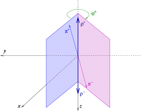
Figure 1: Definition of the $\rho^{+}\rho^{-}$ decay products’ acoplanarity distribution angle $\varphi^{*}$, in the rest frame of the $\rho^{+}\rho^{-}$ pair. The range for $\varphi^{*}$ is $0\leq\varphi^{*}\leq 2\pi$. Note that, for better visualization, we use in this figure the momenta of $\pi^{\pm}$ and $\rho^{\pm}$ (rather than $\pi^{0}$’s from $\rho^{\pm}$ decays) to define the planes. The two ways of defining the planes are equivalent if no reconstruction errors are taken.

4 The Monte Carlo

If any non-zero CP-odd admixture to the Higgs is present, not only is the distribution of the Higgs decay products modified, but also the distribution of its production angle [10, 11, 12]. In this paper, we simulate production angular distributions as in the SM, but this assumption has no influence on the validity of the analysis. In particular, the detection efficiencies for pure CP-even and pure CP-odd Higgs bosons do not differ significantly. In order to study the sensitivity of $h\to\tau^{+}\tau^{-}$ observables, we assume a production rate independent of the size of the CP-odd admixture, i.e. the SM production rate of a CP-even Higgs.

The production process $e^{+}e^{-}\to Zh\to\mu^{+}\mu^{-}(q\bar{q})\tau^{+}\tau^{-}$ has been chosen, as an representative example, and simulated with the Monte Carlo program PYTHIA 6.1 [13]. The Higgs boson mass of 120 GeV and a center-of-mass energy of 350 GeV was chosen. The effects of initial state bremsstrahlung were included. For the sake of our discussion and in all of our samples the $\tau$ decays have been generated with the TAUOLA Monte Carlo library [3, 4, 5]. As usual, to facilitate the interpretation of the results, bremsstrahlung effects in decays were not taken into account. Anyway, with the help of additional simulation, we have found this effect to be rather small. To include the full spin effects in the $h\to\tau^{+}\tau^{-}$, $\tau^{\pm}\to\rho^{\pm}\bar{\nu}_{\tau}(\nu_{\tau})$, $\rho^{\pm}\to\pi^{\pm}\pi^{0}$ decay chain, the interface explained in Ref. [6] was used, with the extensions discussed in Section 2.

5 Idealized results

5.1 Resolution parameters

To test the feasibility of the measurement, some assumptions about the detector effects had to be made. We include, as the most critical for our discussion, effects due to inaccuracies in the measurement of the $\pi^{\pm},\pi^{0}$ momenta and of the $\tau^{\pm}$ leptons impact parameters. We assumed Gaussian spreads of the measured quantities with respect to the generated ones and we used the following algorithm to reconstruct the energies of $\pi$’s in their respective $\tau^{\pm}$ rest frames, exactly as in the case of the studies presented in Refs. [8, 9].

1. Charged-pion momentum: We assume a 0.1% spread on its energy and direction.

2. Neutral-pion momentum: We assume an energy spread of $5\%\over\sqrt{E[{\rm GeV}]}$. For the $\theta$ and $\phi$ angular spread we assume ${1\over 3}{2\pi\over 1800}$. These $\pi^{0}$ resolutions can be achieved with a 15% energy error and a 2$\pi$/1800 direction error in the gammas resulting from the $\pi^{0}$ decays. These resolutions have been approximately verified with SIMDET [14], a parametric Monte Carlo program for TESLA detector [15], as well as with other studies, see e.g. Refs. [16, 17].

3. The reconstructed Higgs boson rest frame: We assume a spread of $2$ GeV with respect to the transverse momentum of the reconstructed Higgs boson momentum, and $5$ GeV for the longitudinal component, to mimic the beamstrahlung effect.

4. The impact parameter: The angular resolution of the $\tau$ impact parameter has been simulated for a TESLA-like detector. The simulation is based on the anticipated performance of a 5-layer CCD vertex detector, as described in Ref. [15]. For Higgsstrahlung events with $h_{SM}\to\tau^{+}\tau^{-}$ and $\tau^{\pm}\to\rho^{\pm}\bar{\nu}_{\tau}(\nu_{\tau})$ at $m_{h_{SM}}=$ $120$ GeV and $\sqrt{s}=$ $350$ GeV, the angular resolution has been found [9] to be approximately 25^∘.

5.2 Numerical results

We have used the scalar–pseudoscalar mixing angle $\phi=\frac{\pi}{4}$ and, as the reference, we have used the pure scalar case $\phi=0$.

In Fig. 2 the acoplanarity distribution angle $\varphi^{*}$ of the $\rho^{+}\rho^{-}$ decay products which was defined in the rest frame of the reconstructed $\rho^{+}\rho^{-}$ pair, is shown. Unobservable generator-level $\tau^{\pm}$ rest frames are used for the calculation of selection cuts. The two plots represent events selected by the differences of $\pi^{\pm}\pi^{0}$ energies, defined in their respective $\tau^{\pm}$ rest frames. In the left plot, it is required that $y_{1}y_{2}>0$, whereas in the right one, events with $y_{1}y_{2}<0$ are taken. This figure quantifies the size of the parity effect in an idealized condition, which we will attempt to approach with realistic ones. The size of the effect was substantially diminished when a detector-like set-up was included for $\tau^{\pm}$ rest frames reconstruction as well, see Fig. 3, in exactly the same proportion as in Ref. [8]. The general shape of the distributions remained.

At the cost of introducing cuts, and thus reducing the number of accepted events, we could achieve some improvement of the method, as in Ref. [9]. If we require the signs of the reconstructed energy differences $y_{1}$ and $y_{2}$ (Eq. (8)) to be the same whether the method is used with or without the help of the $\tau$ lepton impact parameter, only $\sim 52\%$ of events are accepted. The relative size of the parity effect increases. Results are presented in Fig. 3.

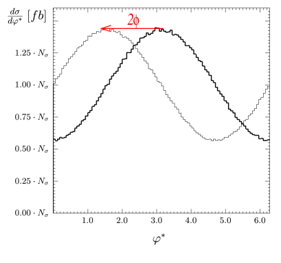
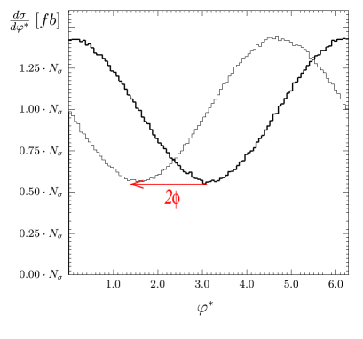
Figure 2: The acoplanarity distribution (angle $\varphi^{*}$) of the $\rho^{+}\rho^{-}$ decay products in the rest frame of the $\rho^{+}\rho^{-}$ pair. Gaussian smearing of $\pi$’s momenta as described in Section 5.1 is included. However, generator level $\tau^{\pm}$ rest frames are used. The thick line corresponds to a scalar Higgs boson, the thin line to a mixed one. The left figure contains events with $y_{1}y_{2}>0$, the right one is for $y_{1}y_{2}<0$. In our paper, that is for the 350 GeV $e^{+}e^{-}$ CMS (scalar 120 GeV mass) Higgsstrahlung production we took $N_{\sigma}=62.7\cdot 10^{-3}\;[fb]$ for the scale of the plot. In general case $N_{\sigma}=\frac{1}{4\pi}\sigma_{total}(e^{+}e^{-}\to XH){\cal BR}(H\to\tau^{+}\tau^{-})\bigl{(}{\cal BR}(\tau\to\rho\nu_{\tau})\bigr{)}^{2}$ is a suitable choice.

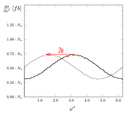
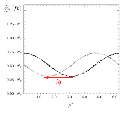
Figure 3: The acoplanarity distribution (angle $\varphi^{*}$) of the $\rho^{+}\rho^{-}$ decay products in the rest frame of the $\rho^{+}\rho^{-}$ pair. Gaussian smearing of $\pi$’s and Higgs boson momenta, as described in Section 5.1 is included. Only events where the signs of the energy differences $y_{1}$ and $y_{2}$ are the same, if calculated using the method described in Ref. [8] and if calculated with the help of the $\tau$ impact parameter Ref. [9], are taken. The thick line corresponds to a scalar Higgs boson, the thin line to a mixed one. The left figure contains events with $y_{1}y_{2}>0$, the right one is for $y_{1}y_{2}<0$. In our paper, that is for the 350 GeV $e^{+}e^{-}$ CMS (scalar 120 GeV mass) Higgsstrahlung production we took $N_{\sigma}=62.7\cdot 10^{-3}\;[fb]$ for the scale of the plot. In general case $N_{\sigma}=\frac{1}{4\pi}\sigma_{total}(e^{+}e^{-}\to XH){\cal BR}(H\to\tau^{+}\tau^{-})\bigl{(}{\cal BR}(\tau\to\rho\nu_{\tau})\bigr{)}^{2}$ is a suitable choice.

6 Simulation with detector effects

In order to assess the possibilities for a measurement of the acoplanarity distribution described in Section 2, we perform a detailed simulation of Higgs bosons produced in the Higgsstrahlung process using PYTHIA 6.2 [13] for the production process and the modified version of TAUOLA described above to generate samples of signal events. These events are then passed through a simulation of the TESLA detector (SIMDET [14]) accounting for the acceptance and anticipated resolution of the tracking devices and calorimeters corresponding to the detector proposed in the TESLA TDR [15].

Signal samples of 1 ab^-1 at 350 GeV center-of-mass energy were generated for scalar–pseudoscalar mixing angles $\phi=0$, $\pi/8$ and $\pi/4$. With detector simulation the $\tau$ leptons decaying to $\pi^{\pm}\pi^{0}$ from Higgs decays were reconstructed as isolated jets with only one charged track (the reconstructed $\pi^{\pm}$) and additional neutral clusters (the reconstructed $\pi^{0}$). The $\pi^{\pm}$ and $\pi^{0}$ momenta were combined to form a reconstructed $\rho^{\pm}$. The acoplanarity angle $\varphi^{*}$ was calculated in the reconstructed $\rho^{+}\rho^{-}$ rest frame. Two event classes are formed according to the sign of $y_{1}y_{2}$, where $y_{1}$ and $y_{2}$ are calculated in the laboratory frame. The resulting $\varphi^{*}$ distributions for the three $\phi$ cases are shown in Fig. 4 as histograms, each containing about 0.5 ab^-1 statistics.

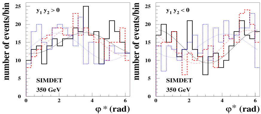
Figure 4: Distribution of the reconstructed acoplanarity angle $\varphi^{*}$ for $\phi=0$ (full histogram), $\phi=\pi/8$ (dashed histogram) and $\phi=\pi/4$ (dotted histogram) for $y_{1}y_{2}>0$ (left) and $y_{1}y_{2}<0$ (right). The lines indicate the results of the corresponding fits (see text).

To extract the scalar–pseudoscalar mixing angles $\phi$ the functions $a*\cos(\varphi^{*}-2\phi)+b$ (for $y_{1}y_{2}>0$) and $a*\cos(\varphi^{*}-2\phi+\pi)+b$ (for $y_{1}y_{2}<0$) were used to fit 2$\phi$ to the reconstructed acoplanarities $\varphi^{*}$, gained from simulated detector signals. The constants $a$ and $b$ were additional free variables of the 3-parameter fit. The resulting functions are also shown as lines in Fig. 4.

In order to assess the expected accuracy and a possible experimental bias of the $\phi$ measurement, the above procedure was repeated 400 times with acoplanarity distributions extracted from independent samples of 1 ab^-1 luminosity each, with a nominal value of $\phi=\pi/4$. Unlike what was done before in Fig. 4, the data for the two ranges of value of $y_{1}y_{2}$ were appropriately combined into one $\varphi^{*}$ distribution before the fit. The new value of $\varphi^{*}$ for the case of $y_{1}y_{2}<0$ had to be redefined as $\varphi^{*}+\pi$ for $0<\varphi^{*}<\pi$ and $\varphi^{*}-\pi$ for $\pi<\varphi^{*}<2\pi$. The distribution of the fit results on $2\phi$ for each of the experiments is shown in Fig. 5. The mean value is $1.627\pm 0.014$, compared to the $\frac{\pi}{2}$ input value. The resulting bias of approximately 3^∘ can probably be corrected in the future. The expected error on $2\phi$ is obtained as the width of this distribution. It amounts to $0.20\pm 0.01$ rad, or approximately 12^∘. Thus, a precision on $\phi$ of approximately 6^∘ can be anticipated for a SM Higgs cross section and $h\to\tau^{+}\tau^{-}$ branching ratio at $\sqrt{s}=350$ GeV and 1 ab^-1. Note that so far backgrounds neither from other Higgs boson decays nor from other SM processes have been considered. While previous studies [19] have shown that $h\to\tau^{+}\tau^{-}$ events can be selected without large backgrounds, some small deterioration and a further lowered signal efficiency are to be expected. Because of the small observed bias, it is not expected that systematic effects will limit the resolution even for production cross sections a few times larger than in the SM.

7 Conclusions

We have found that for an integrated luminosity of 1 ab^-1, at 350 GeV center-of-mass energy, a high precision LC detector such as the proposed TESLA, should be able to measure the scalar–pseudoscalar mixing angle for the $h\tau\tau$ coupling with 6^∘ accuracy in the case of a Standard Model Higgs boson of 120 GeV mass. The experimental error is expected to be dominated by statistics.

However, if the production mechanism of the Higgs boson happened to be non-SM and larger, the systematic errors not studied so far and possible new, unknown phenomena may have some significant influence. On the basis of studies performed to date, we believe however that, if the cross section were somewhat larger than the Standard Model one and thus the uncertainty on the mixing angle due to statistics were not smaller than 4^∘, we do not expect the systematic error to be a problem. In the case of Higgs boson scenarios predicting even higher rates of observed $h\to\tau\tau$ samples, the issue of the systematic error definitely needs to be re-addressed before any conclusion on measuring the scalar–pseudoscalar mixing angle in the $h\tau\tau$ coupling with higher precision can be attempted.

Finally, let us note that this method can be applied to measure the parity properties of other scalar particles, not necessarily only Higgs boson(s).

Figure 5: Distribution of the fit values for $2\phi$ from 400 independent samples, each corresponding to a luminosity of 1 ab^-1, for a generated value of $\phi=\pi/4$. The curve represents the fit of a Gaussian to this distribution. Its width represents the expected statistical error on $2\phi$.

Acknowledgements

Two of us (ZW and MW) would like to thank M. Peskin for raising, two years ago, our attention to the importance of measuring, at LC, the parity of the Higgs boson using the $\tau\tau$ decay channel.

References

- [1] T. Pierzchała, E. Richter-Wa̧s, Z. Wa̧s, and M. Worek, Acta Phys. Polon. B32 (2001) 1277–1296, hep-ph/0101311.
- [2] M. Worek, Acta Phys. Pol. B32 (2001) 3803–3811, hep-ph/0110228.
- [3] S. Jadach, J. H. Kühn, and Z. Wa̧s, Comput. Phys. Commun. 64 (1990) 275.
- [4] M. Jeżabek, Z. Wa̧s, S. Jadach, and J. H. Kühn, Comput. Phys. Commun. 70 (1992) 69.
- [5] S. Jadach, Z. Wa̧s, R. Decker, and J. H. Kühn, Comput. Phys. Commun. 76 (1993) 361.
- [6] Z. Wa̧s and M. Worek, Acta Phys. Polon. B33 (2002) 1875, hep-ph/0202007.
- [7] M. Worek, Acta Phys. Polon. B34 (2003) 4549, hep-ph/0305082.
- [8] G. R. Bower, T. Pierzchała, Z. Wa̧s, and M. Worek, Phys. Lett. B543 (2002) 227, hep-ph/0204292.
- [9] K. Desch, Z. Wa̧s and M. Worek, Eur. Phys. J. C29 (2003) 491, hep-ph/0302046.
- [10] American Linear Collider Working Group Collaboration, T. Abe et al., page 123 and references therein., hep-ex/0106056.
- [11] M. Kramer, J. H. Kühn, M. L. Stong, and P. M. Zerwas, Z. Phys. C64 (1994) 21, hep-ph/9404280.
- [12] B. Grzadkowski and J. F. Gunion, Phys. Lett. B350 (1995) 218, hep-ph/9501339.
- [13] T. Sjöstrand et al., Comput. Phys. Commun. 135 (2001) 238, hep-ph/0010017.
- [14] M. Pohl and H. J. Schreiber, “SIMDET - Version 4: A parametric Monte Carlo for a TESLA detector”, hep-ex/0206009.
- [15] T. Behnke, S. Bertolucci, R. D. Heuer, and R. Settles, “TESLA Technical Design Report Part IV: A detector for TESLA”, DESY-01-011.
- [16] G. R. Bower, “Proceedings of the Worldwide Study on Physics and Experiments with Future Linear Colliders” (1999) 1049.
- [17] G. R. Bower, “Physics and Experiments with Future Linear Colliders LCWS 2000” (2000) 920.
- [18] J. A. Aguilar-Saavedra et al., “TESLA Technical Design Report Part III: Physics at an Linear Collider”, hep-ph/0106315.
- [19] J. C. Brient, LC Note LC-PHSM-2002-003 (2002).