Models of quintessence coupled to the electromagnetic field and the cosmological evolution of alpha

Abstract

We study the change of the effective fine structure constant in the cosmological models of a scalar field with a non-vanishing coupling to the electromagnetic field. Combining cosmological data and terrestrial observations we place empirical constraints on the size of the possible coupling and explore a large class of models that exhibit tracking behavior. The change of the fine structure constant implied by the quasar absorption spectra together with the requirement of tracking behavior impose a lower bound of the size of this coupling. Furthermore, the transition to the quintessence regime implies a narrow window for this coupling around $10^{-5}$ in units of the inverse Planck mass. We also propose a non-minimal coupling between electromagnetism and quintessence which has the effect of leading only to changes of alpha determined from atomic physics phenomena, but leaving no observable consequences through nuclear physics effects. In doing so we are able to reconcile the claimed cosmological evidence for a changing fine structure constant with the tight constraints emerging from the Oklo natural nuclear reactor.

1 Introduction

Recently claimed observational evidence for a $\sim$ 10ppm change of the fine structure constant over cosmological time between $z\simeq 0.5$ and $z=0$ brings an unexpected and interesting support to the old idea of Dirac Dirac . The result of Webb et al. Webb01 (if it continues to defy alternative explanations by systematic effects Murphy:2002ve ) has serious implications for cosmology, astrophysics and particle physics, Sister -Bek02 .

The most powerful conclusion that follows from Webb01 is the existence of new fields, massless or nearly massless, and different from gravitation, electromagnetism, neutrinos and axions. Indeed, the “promotion” of a coupling constant $g$ into a function of time immediately implies that it should also depend on the rest of the coordinates, $g=g(x)$. The dependence of $g$ on $x$ in an interacting theory will inevitably generate a kinetic term $\partial_{\mu}g\partial^{\mu}g$, so that the “coupling constant” becomes a propagating field. In order to avoid confusing terminology of “changing alpha”, it is reasonable to introduce a new degree of freedom, a scalar field $\phi(x)$, via a chain of relations:

$$\frac{1}{g^{2}}F_{\mu\nu}F^{\mu\nu} ~{}\longrightarrow~{} \frac{1}{g^{2}(t)}F_{\mu\nu}F^{\mu\nu}~{}\longrightarrow~{}$$

$$\frac{1}{g^{2}(x)}F_{\mu\nu}F^{\mu\nu} ~{}\longrightarrow~{} \frac{1}{g^{2}_{0}}B_{F}(\phi(x))F_{\mu\nu}F^{\mu\nu}\,.$$

We postulate that the scalar field couples to the electromagnetic $F_{\mu\nu}F^{\mu\nu}$ via some unknown dimensionless function $B_{F}(\phi(x))$. Using the freedom in the definition, one can always choose $B_{F}(\phi(z=0))=1$, so that $g_{0}$ is the coupling constant “today”, i.e. at the redshift $z=0$.

The dependence of gauge coupling constants on coordinates can hardly be regarded as a theoretical novelty. Indeed, in string theory/supergravity all effective coupling constants depend on scalar field(s) $\phi_{i}(x)$, so that $g=g(\phi_{i}(x))$. However, the late change of $g$, a few billion years after the Big Bang, implies that some of these fields have essentially near flat potentials, i.e. their masses must be comparable to the Hubble parameter at the present epoch $\sim 10^{-32}$ eV. This is in contrast with the phenomenologically developed models of string theory/supergravity, where all moduli are believed to receive electroweak scale masses after supersymmetry breaking, which makes them completely frozen long before nucleosynthesis, not mentioning the present epoch. Therefore, such a late evolution of the effective $\alpha$ comes as a total surprise for particle physics.

In general, a nearly massless scalar poses a serious problem of naturalness, which only worsens if this scalar is interacting BDD . Indeed, the inclusion of a non-renormalizable interaction of the form $B_{F}(\phi)F^{2}$ at the quantum level requires the existence of a momentum cut-off $\Lambda_{UV}$. Unfortunately,, any particle physics motivated choice of $\Lambda_{UV}$ destabilizes the quintessence potential, i.e. it could induce a mass term much larger than the required $m_{\phi}\sim H_{0}$. However, because the nature of this fine-tuning is similar to the one required for the smallness of the cosmological constant, we choose to proceed hoping that one day both problems could be resolved simultaneously.

The study of the interaction (LABEL:tx) has a long history. Initially, it was examined by Bekenstein Bek , who introduced the exponential form for the coupling of the scalar field to the electromagnetic Lagrangian which in practice can always be taken in the linear form $B_{F}(\phi(x))=1-\zeta\kappa\phi$, where $\kappa^{2}=8\pi G$. He showed that the exchange by this scalar leads to the effective non-universality of the gravitational force which bounds the possible size of $\zeta$ at one per mil level. The cosmological evolution of $\phi$ is dynamical and it starts immediately after the transition to a matter-dominated Universe. In principle, the existence of a non-zero $\zeta$ alone is sufficient to ensure the cosmological evolution of $\phi$, driven by the electromagnetic portion of the baryon mass density. However, in the minimal Bekenstein model where $\zeta$ is the only source for $\phi$, the resulting change of $\alpha$ is way too small to be interesting: $|\alpha(z\sim 1)-\alpha_{0}|/\alpha_{0}\mathrel{\raise 1.29167pt\hbox{$<$\kern-7.5pt\lower 4.30554pt\hbox{$\sim$}}}10^{-10}-10^{-9}$ Bek ; LS ; OP An enhancement by up to five-six orders of magnitude may occur by abandoning the minimalistic approach and introducing a “generalized” Bekenstein model where $\phi$ is driven either by $O(1)$ couplings to dark matter or by its own potential OP ; SBM , in which case $\Delta\alpha/\alpha$ may be consistent with the results of Refs. Webb01 .

Quite independently from the physics of changing couplings, there has been a tremendous increase of interest towards cosmological models with a light scalar field as a possible source of dark energy or quintessence. Evidence for the change of the effective coupling constant is a strong argument in favor of the existence of a scalar field with the wave length comparable to the size of the Universe which thus makes it a good candidate for quintessence. Even though the concept of quintessence and the choice if its potential looks completely ad hoc, some quintessence models have an advantage over a “simple” explanation of dark energy by a non-zero cosmological constant. Indeed, certain forms of potentials allow for an attractor-type solution, in which case the late cosmological evolution of $\phi$ has no memory of the initial conditions that could be chosen (almost) arbitrarily. The evolution of the energy density of the $\phi$ field is subdominant with respect to the energy density of matter and radiation, and only during the last stages of the cosmological evolution does it become a dominant component. It is thus intriguing to identify the field $\phi$ responsible for the time dependence of $\alpha$ with tracking quintessence and study possible patterns for $\Delta\alpha/\alpha$ as a function of cosmological time.

In this paper, we present a thorough analysis of a large class of scalar field models with tracking behavior supplemented by a coupling to the electromagnetic field. A similar, but more restricted comparison has recently been made in AG . Where appropriate we will compare our results to those.

A successful model must satisfy the following present constraints:

• Oklo natural reactor $(z=0.14)$ Oklo ; DD ; Fujii ; OPQ :

  $$\left|\frac{\Delta\alpha}{\alpha}\right|\mathrel{\raise 1.29167pt\hbox{$<$\kern-7.5pt\lower 4.30554pt\hbox{$\sim$}}}10^{-7}\,;$$ (1.2)

• Decay rate ${}^{187}{\rm Re}~{}\rightarrow~{}^{187}{\rm Os}$, $(z=0.45)$ OPQ :

  $$\left|\frac{\Delta\alpha}{\alpha}\right|\mathrel{\raise 1.29167pt\hbox{$<$\kern-7.5pt\lower 4.30554pt\hbox{$\sim$}}}10^{-6}\,;$$ (1.3)

• Cosmic microwave background radiation $(z=10^{3})$ Avelino:2001nr :

  $$\left|\frac{\Delta\alpha}{\alpha}\right|<10^{-2}\,;$$ (1.4)

• Big Bang nucleosynthesis $(z=10^{8}-10^{10})$ Ichikawa:2002bt :

  $$\left|\frac{\Delta\alpha}{\alpha}\right|\mathrel{\raise 1.29167pt\hbox{$<$\kern-7.5pt\lower 4.30554pt\hbox{$\sim$}}}2\times 10^{-2}\,;$$ (1.5)

• Atomic clocks $(z=0)$ Marion:2002iw :

  $$\left|\frac{\dot{\alpha}}{\alpha}\right|<4.2\times 10^{-15}~{}{\rm yr}^{-1}\,,$$ (1.6)

  where a dot represents differentiation with respect to cosmic time;

• Equivalence principle tests OP :

  $$|\zeta|<10^{-3}\,.$$ (1.7)

In addition, we take into account the claimed evidence for the variation of the fine structure constant. We will assume

• Quasar absorption lines $(z=3)$ Webb01 :

  $$\frac{\Delta\alpha}{\alpha}=-10^{-5}\,.$$ (1.8)

We first address a minimal Bekenstein-like coupling and find the behavior of the fine structure constant as a function of the redshift for the exponential, power-like and exponential times power-like potentials.

In all cases we analyze the scalar field evolution in the tracking regime i.e., when the energy density of the scalar field remains sub dominant. In this case we are able to present the lower bound on $\zeta$ consistent with tracking behavior and a non-zero change of the fine structure constant Webb01 . The upper limit in this case is furnished by the direct experimental limit on the non-universality of the gravitational force. As a separate exercise, we consider a scalar field as quintessence, i.e. when the tracking regime changes to the scalar field domination at $z\sim 1$. In this case, we are able to determine the allowed window for $\zeta$, without referring to the constraints from the non-universal gravitational forces. Also in the context of a quintessence model, we consider the case of the tracker field driven by the combination of the self potential and the coupling to dark matter.

We confront the predictions for $\Delta\alpha/\alpha$ with the above limits from various astronomical and terrestrial observations, and find that the present day limits on $\dot{\alpha}/\alpha$ and constraints from the Big Bang nucleosynthesis are generally safe. On the other hand, the $\Delta\alpha/\alpha$ coming from the Oklo natural reactor Oklo ; DD ; Fujii ; OPQ and from the meteoritic abundance data OPQ are generally inconsistent with tracking behavior. In the case of a non-minimal coupling of quintessence to the electromagnetic field, the results lose their predictivity as almost any profile for $\alpha(t)$ can be achieved by an appropriate choice of $B_{F}(\phi)$.

We go on to discuss a novel possibility that the effective change of the coupling constant occurs only in atomic interactions while $\Delta\alpha/\alpha$ remains effectively zero for nuclear physics phenomena. The construction we propose is based on the idea that the coupling between photons and the scalar field may change for off-shell photons and has a form factor at some energy above the electron mass. This leads to the suppression of the coupling between the scalar field and the nuclear levels giving a chance to reconcile the results of Webb et al. and the bounds coming from Oklo phenomenon without fine-tuning.

This paper is organized as follows: in the next section we analyze in detail four types of tracking scalar fields and determine the allowed values for $\zeta$. Section 3 addresses the issue of the non-minimal $B_{F}(\phi)$ and introduces the model where $\zeta$ has a form factor. We reach our conclusions is section 4.

2 Minimal coupling of quintessence to the electromagnetic field

We study a class of models of a neutral scalar field coupled to electromagnetism:

$$S= - \frac{1}{2\kappa^{2}}\int d^{4}x\sqrt{-g}~{}R$$ (2.9)

$$+ \int d^{4}x\sqrt{-g}~{}({\cal L}_{\phi}+{\cal L}_{B}+{\cal L}_{\phi F})\,,$$

where $R$ is the scalar curvature. In this paper, we deal with the cosmological evolution and take the stress-energy tensor of the matter fields in a homogeneous form corresponding to a background perfect fluid with the energy-momentum tensor given by

$${T_{B}}_{\mu\nu} \equiv \frac{2}{\sqrt{-g}}\frac{\delta(\sqrt{-g}{\cal L}_{B})}{\delta g^{\mu\nu}}$$ (2.10)

$$= (\rho_{B}+p_{B})u^{\mu}u^{\nu}-g_{\mu\nu}p_{B}\,.$$

Throughout the paper, we employ $(+,-,-,-,)$ signature for the metric tensor. The pressure $p_{B}$ and energy density $\rho_{B}$ are related by the equation of state $p_{B}=(\gamma-1)\rho_{B}$. $\gamma$ is taken to be a constant (e.g. $\gamma=4/3$ for radiation and $\gamma=1$ for matter). The Lagrangian density for the scalar field $\phi$ is

$${\cal L}_{\phi}=\frac{1}{2}\partial^{\mu}\phi\partial_{\mu}\phi-V(\phi)\,.$$ (2.11)

The associated energy-momentum tensor of the scalar field then reads

$${T_{\phi}}_{\mu\nu}=\partial_{\mu}\phi\partial_{\nu}\phi-g_{\mu\nu}\left(\frac{1}{2}\partial^{\mu}\phi\partial_{\mu}\phi-V(\phi)\right)\,.$$ (2.12)

The interaction term between the scalar field and the electromagnetic field is

$${\cal L}_{\phi F}=-\frac{1}{4}B_{F}(\phi)F_{\mu\nu}F^{\mu\nu},$$ (2.13)

where $B_{F}(\phi)$ allows for the evolution in $\phi$. In this paper we adopt a linear dependence on $\phi$ such that $B_{F}(\phi)=1-\zeta\kappa(\phi-\phi_{0})$, where the subscript 0 represents the present value of the quantity. The effective fine structure constant depends on the value of $\phi$ as $\alpha=\alpha_{0}/B_{F}(\phi)$. Therefore, we have

$$\frac{\Delta\alpha}{\alpha}\equiv\frac{\alpha-\alpha_{0}}{\alpha_{0}}=\zeta\kappa(\phi-\phi_{0})\,.$$ (2.14)

We will consider a spatially flat Friedmann-Robertson-Walker (FRW) Universe with metric $ds^{2}=dt^{2}-a^{2}(t)d{\bf x}^{2}$. We further assume a nearly homogeneous scalar field so that the spatial derivatives of the field can be neglected. Hence, we can define analogously to the case of a perfect fluid, the energy density and pressure of a scalar field as, $\rho_{\phi}=\dot{\phi}^{2}/2+V$ and $p_{\phi}=\dot{\phi}^{2}/2-V$, respectively.

The governing equations of motion are

$$\dot{H} = -\frac{\kappa^{2}}{2}\left(\gamma\rho_{B}+\dot{\phi}^{2}\right)\,,$$ (2.15)

$$\dot{\rho}_{B} = -3\gamma H\rho_{B}\,,$$ (2.16)

$$\ddot{\phi} = -3H\dot{\phi}-\frac{dV}{d\phi}\,,$$ (2.17)

subject to the Friedmann constraint

$$H^{2}=\frac{\kappa^{2}}{3}\left(\rho_{B}+\rho_{\phi}\right)\,.$$ (2.18)

The term ${\cal L}_{\phi F}$ can be neglected in the equations determining the dynamics of $\phi$ as its average is zero for photons, and also quite small, $O(10^{-3})$ for baryons Bek ; OP . A notable exception is when $\phi$ couples strongly and directly to dark matter OP .

In the following subsections we will consider different forms of the scalar potential $V(\phi)$ and analyze two possible cases of evolution of the field: (i) slow roll down the potential $V(\phi)$ controlled by the friction provided by the background fluid (tracker evolution); (ii) the field provides the source of dark energy, and is just starting to dominate the dynamics leading the universe into a period of accelerated expansion. We will start by estimating the value of the coupling $\zeta$ consistent with Eq. (1.8) by setting

$$\zeta=-\frac{10^{-5}}{\kappa\phi(z=3)-\kappa\phi(z=0)}\,.$$ (2.19)

One should bare in mind that we are not attempting to fit the data to specific scalar potentials but instead to extract an estimate of $\zeta$ consistent with the data.

We calculate the ratio of the variation of $\alpha$ with time at present using the relation

$$\frac{\dot{\alpha}}{\alpha}=-\zeta\frac{d(\kappa\phi)}{d(1+z)}~{}H_{0}\,,$$ (2.20)

where $H_{0}$ is the value of the Hubble constant today, $H_{0}=h/9.78~{}\times 10^{-9}~{}{\rm yr}^{-1}$. We will use $h=0.65$ throughout the paper.

2.1 Exponential potentials

For a pure exponential potential $V(\phi)=V_{0}\exp(-\lambda\kappa\phi)$, there exist just two possible late time attractor solutions with quite different properties, depending on the values of $\lambda$ and the background’s equation of state $\gamma$ Copeland:1997et :

(1) $\lambda^{2}>3\gamma$. The late time attractor is one where the scalar field mimics the evolution of the barotropic fluid with $\gamma_{\phi}=\gamma$, and the relation $\Omega_{\phi}=3\gamma/\lambda^{2}$ holds.

(2) $\lambda^{2}<3\gamma$. The late time attractor is the scalar field dominated solution ($\Omega_{\phi}=1$) with $\gamma_{\phi}=\lambda^{2}/3$.

The second regime can be discarded as unrealistic. Indeed, there is a tight constraint on the allowed magnitude of $\Omega_{\phi}$ at the time of Big Bang nucleosynthesis, $\Omega_{\phi}(1~{}{\rm MeV})<0.045$ Bean:2001wt . Moreover, we must allow time for the formation of structure before the universe starts accelerating, which requires $\Omega_{\phi}$ to be subdominant after the CMB decoupling. Therefore, the transition to $\Omega_{\phi}\simeq 1$ should occur at the present epoch. For this model, this is possible only at the expense of extreme fine tuning of the initial value $\rho_{\phi}^{\rm in}$, a type of fine-tuning that goes against the whole idea of the tracker/quintessence field. The first regime is perfectly compatible with all experimental data, if there is an additional component to dark energy which ensures the late time acceleration, as the $\phi$ field itself in this model does not allow for an accelerating expansion.

For now we simply assume that the scalar field responsible for the change in the value of $\alpha$ is tracking and is subdominant today, i.e. $\Omega_{\phi}<1/2$. This imposes a lower bound $|\lambda|\geq\sqrt{6}$. The evolution of the field in the tracker regime is well known and is given by Ng:2001hs

$$\kappa(\phi-\phi_{0})=-\frac{3\gamma}{\lambda}\ln(1+z)\,.$$ (2.21)

Therefore, combining Eqs. (2.19) and (2.21), we obtain

$$\zeta=\frac{10^{-5}}{\ln(4)}~{}\frac{\lambda}{3\gamma}\,.$$ (2.22)

As we discussed before, if $\rho_{\phi}$ is subdominant today, then there must be some other source of dark energy responsible for the accelerating universe. The presence of a cosmological constant introduces an error of less than $30\%$ in the above estimate. With $|\lambda|$ being limited from below, this imposes the lower bound on the possible size of the coupling, $\zeta>6\times 10^{-6}$. On the other hand, $\zeta$ is limited from tests of the equivalence principle, $|\zeta|<10^{-3}$, which we can use to further constrain the value of the parameter $\lambda$ in a matter dominated universe:

$$\sqrt{6}<|\lambda|<415\,.$$ (2.23)

From Eq. (2.20) we immediately extract that for this potential $\dot{\alpha}/\alpha=4.8\times 10^{-16}~{}{\rm yr}^{-1}$ consistent with the atomic clocks bound Eq. (1.6).

It is also instructive to check whether this range of couplings is consistent with constraints on $\Delta\alpha/\alpha$ coming from the Big Bang nucleosynthesis. In the radiation dominated era, the evolution of the scalar field is given by

$$\kappa(\phi-\phi_{0})=-\frac{3}{\lambda}\ln(1+z_{\rm eq})-\frac{4}{\lambda}\ln\left(\frac{1+z}{1+z_{\rm eq}}\right)\,,$$ (2.24)

where $1+z_{\rm eq}$ is the redshift at which the energy density of the radiation and matter components have the same value, $z_{\rm eq}=\Omega_{\rm M}^{0}/\Omega_{\rm R}^{0}\approx 5\times 10^{3}$. Substituting into Eq. (2.14) for the estimated value of $\zeta$, it is easy to verify that $\Delta\alpha/\alpha=-2\times 10^{-4}$ at redshift $z=10^{10}$, which is fully consistent with the bound in Eq. (1.5).

2.2 Power law potentials

For an inverse power law potential of the form $V(\phi)=M^{4+n}/\phi^{n}$ the cosmological evolution of the field is given by Ng:2001hs

$$\kappa(\phi-\phi_{0})=\kappa\phi_{0}\left[-1+(1+z)^{-3\gamma/(2+n)}\right]\,,$$ (2.25)

where the value of $\phi$ at $z=0$ is given by

$$\phi_{0}=\left[\frac{3}{2}\frac{\kappa^{2}\rho_{B}^{0}}{M^{4+n}}\frac{1}{n^{2}}\frac{\gamma n}{n+2}\left(2-\frac{\gamma n}{n+2}\right)\right]^{-1/(2+n)}\,.$$ (2.26)

Combining Eq. (2.25) with Eq. (2.19) we can estimate the coupling with electromagnetism through

$$\zeta=-\frac{10^{-5}}{-1+4^{\beta}}~{}(\kappa\phi_{0})^{-1}\,,$$ (2.27)

where $\beta=-3\gamma/(2+n)$.

In Fig. 1 we show a contour plot for $\log\zeta$ as a function of the parameters $n$ and $M$ in the scalar potential consistent with $\Delta\alpha/\alpha$ suggested by the QSO data. A few comments are in order at this point. Note that at fixed $n$, $\zeta$ falls off with increasing $M$. This behavior follows from Eq. (2.26): as the mass scale $M$ increases so does $\phi_{0}$ and consequently $\kappa(\phi-\phi_{0})$. The dashed line on this plot represents the upper bound on the mass scale $M$ coming from our initial assumption that the field is tracking today. For a given $n$, the value of this upper bound corresponds to the case when the field has just begun to dominate. This is the case of quintessence. Moreover, a value larger than this means that the scalar field has been dominating the evolution of the universe for a long time preventing any formation of structure. Thus everything above the dashed line is excluded. The equivalence principle bound, $|\zeta|<10^{-3}$, and the upper bound on $M$ produce an allowed band for the pair $(n,M)$ limited by the contours $-5$ and $-3$ in Fig. 1.

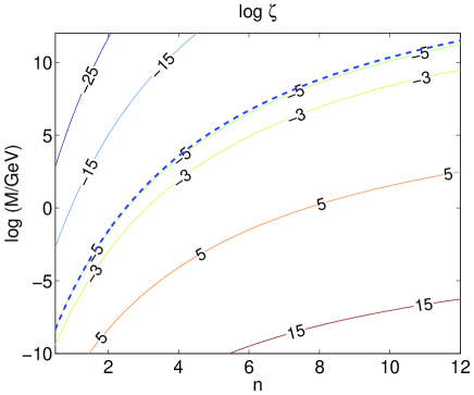
Figure 1: Contour plot for $\log\zeta$ with respect to the possible choices of $n$ and $M$ in the inverse power law potential. The dashed line represents the maximum value for $M$ that allows tracking evolution of the field at present.

The case of quintessence (i.e. along the dashed line in Fig. 1) is more involved and requires a special approach as the field today is no longer in an attractor regime but in the transition between the tracker and a scalar field dominated solution. Nevertheless, from Fig. 1 we expect the value of the coupling to be close to $\zeta\approx 10^{-5}$. In Fig. 2 we show the variation of parameter $\zeta$ with $n$ for a Universe with $\Omega_{\phi}=0.7$ today. This curve was obtained by solving numerically the evolution equations of the field followed by extraction of the coupling $\zeta$ through Eq. (2.19). One should point out that models with $n>3$ lead to an equation of state for the quintessence field in clear disagreement with observations as the latter indicate $\gamma_{\phi}\equiv p_{\phi}/\rho_{\phi}>0.4$ Efstathiou:1999tm . On the other hand, models with $n<1$ do not alleviate the initial conditions problem, which was the great advantage of tracking quintessence models over the bare cosmological constant. Thus, the range of interesting $n$, $1\leq n\leq 3$, in the case of quintessence defines the window of the coupling constant $\zeta$ that agrees with QSO evidence for changing alpha:

$$8.6\times 10^{-6}<\zeta<1.4\times 10^{-5}\,.$$ (2.28)

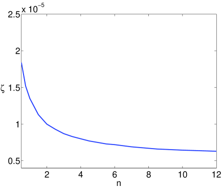
Figure 2: Variation of $\zeta$ with the parameter $n$ for an inverse power law quintessence model.

We can calculate now the value of $\dot{\alpha}/\alpha$ at present for a given $n$ using Eq. (2.20). In Fig. 3 we show the shapes of these curves for the tracker and quintessence cases.

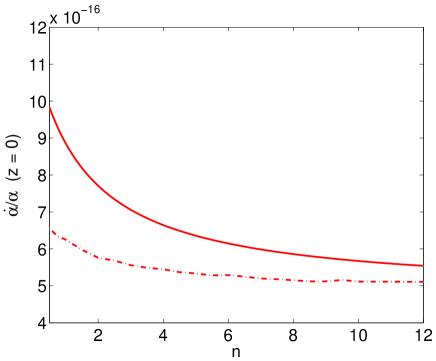
Figure 3: $\dot{\alpha}/\alpha$ at present for a tracker evolution along an inverse power law potential (solid line) and for a quintessence model (dot-dashed line).

Finally, as in the case of the exponential potential, the BBN bounds on $\Delta\alpha$ are satisfied with this model. The evolution of the field in the radiation dominated epoch is

$$\kappa(\phi-\phi_{0})=\kappa\phi_{0}\left[-1+(1+z_{\rm eq})^{-3/(2+n)}~{}\times\right.$$

$$\left.\left(\frac{1+z}{1+z_{\rm eq}}\right)^{-4/(2+n)}\right]\,,$$ (2.29)

hence, we can verify that
$10^{-5}<|\Delta\alpha/\alpha(z=10^{10})|<4\times 10^{-5}$, well within the bound of Eq. (1.5).

2.3 SUGRA type potentials

Let us now consider the more general potential studied in Ref. Ng:2001hs which we write in the form

$$V(\phi)=V_{0}e^{\lambda(\kappa\phi)^{\beta}}(\kappa\phi)^{n}\,.$$ (2.30)

See Refs. Brax:1999gp ; Copeland:2000vh that motivate this form within a supergravity context, hence the name adopted here. For negative $n$ this potential has a minimum with non-vanishing energy density which upon convenient choice of the energy scale $V_{0}$ can explain the present acceleration of the universe. The evolution of the field cannot be written in an explicit form but, for $(\kappa\phi)^{\beta}\gg n/\lambda\beta$ the evolution in the tracker regime can be written in terms of a perturbative solution to order $k$ written recursively, such that

$$\lambda(\kappa\phi)^{\beta}_{(1)} = \Phi_{i}+3\gamma\ln(1+z)\,,$$

$$\lambda(\kappa\phi)^{\beta}_{(k)} = \lambda(\kappa\phi)^{\beta}_{(1)}+\frac{2-n}{\beta}\ln(\kappa\phi)^{\beta}_{(k-1)}$$ (2.31)

$$-2\ln\left[\lambda\beta(\kappa\phi)^{\beta}_{(k-1)}+n\right]\,$$

where

$$\Phi_{i}=\ln\left[\frac{3}{2}\frac{\rho_{B}^{0}}{V_{0}}\gamma(2-\gamma)\right]\,.$$ (2.32)

and the last logarithm term only exists if $\lambda\neq 0$. The case $(\kappa\phi)^{\beta}\ll n/\lambda\beta$ is simply the power law case that we studied in part B.

Following the method adopted above to estimate $\zeta$, its value is given by

$$\zeta=-\frac{10^{-5}}{\kappa\phi_{(k)}(z=3)-\kappa\phi_{(k)}(z=0)}\,,$$ (2.33)

where $\phi_{(k)}$ is given by Eq. (2.3). In Fig. 4 we show a contour plot for the value of $\zeta$ necessary to account for the QSO data, using the second order approximation $k=2$. In the tracker regime we expect a weak dependence of any derived quantities on the parameter $n$. This argument follows from the initial assumption that the field is rolling along the exponential side of the potential. We have fixed $\beta=2$, $n=-11$ and made $\lambda$ and $V_{0}$ free parameters. The particular case $\lambda=1/2$ leads to the form of the potential in Ref. Brax:1999gp . In Fig. 4 we show a contour plot for $\log\zeta$ with respect to the possible choices of $n$ and $V_{0}$. The dashed line represents the value of $V_{0}$ that corresponds to the present energy density of dark energy assuming that the field has already reached the minimum of the potential at $z=0$. This method of estimating $V_{0}$ is particulary good for $\lambda>1$.

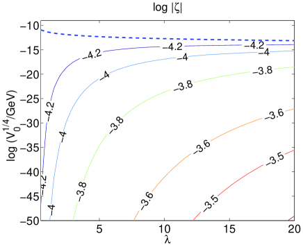
Figure 4: Contour plot for $\log|\zeta|$ with respect to the possible choices of $\lambda$ and $V_{0}$ for the model of Eq. (2.30) with $n=-11$ and $\beta=2$.

As we have seen in the inverse power law potential case, as we approach the dashed line (or quintessence like behavior) the value of the coupling approaches $\zeta\approx 10^{-5}$. For very small values of $V_{0}$ and large $\lambda$ we enter the region of parameters disfavored by the equivalence principle experiments. Again, as in the inverse power law potential, we obtain an allowed band, now for the pair $(\lambda,V_{0})$, limited by the contours $-5$ and $-3$. For increasing $\beta$ one can verify that this band becomes narrower.

To calculate the variation of $\alpha$ at the time of nucleosynthesis we just have to realize that the only modification in Eq. (2.3) is that in the radiation era

$$\lambda(\kappa\phi)^{\beta}_{(1)}=\Phi_{i}+3\ln(1+z_{\rm eq})+4\ln\left(\frac{1+z}{1+z_{\rm eq}}\right)\,.$$ (2.34)

In Figs. 5 and 6 we show that both the values of $\dot{\alpha}/\alpha$ at present and $\Delta\alpha/\alpha$ at nucleosynthesis for this model are within the current experimental and observational bounds. A striking property is that these quantities are extremely insensitive to the values chosen for the parameters of the model, a feature we came across before in the previous models. This should not come as a surprise because when we estimate $\zeta$ by fixing $\Delta\alpha/\alpha=10^{-5}$ at $z=3$, we are effectively demanding that the late time evolution is roughly the same for any choice of parameters.

Figure 5: Contour plot for $\dot{\alpha}/\alpha$ with respect to the possible choices of $\lambda$ and $V_{0}$ for the model of Eq. (2.30) with $n=-11$ and $\beta=2$.

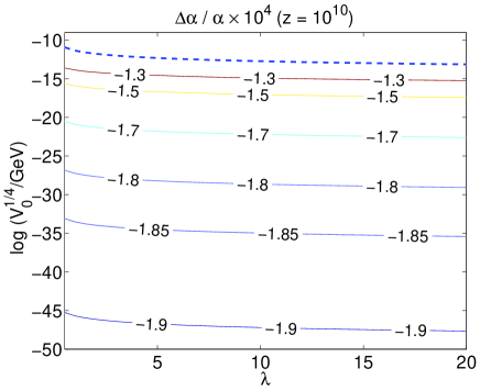
Figure 6: Contour plot for $\Delta\alpha/\alpha$ at nucleosynthesis with respect to the possible choices of $\lambda$ and $V_{0}$ for the model of Eq. (2.30) with $n=-11$ and $\beta=2$.

2.4 Coupled quintessence

We now consider a linear coupling between the scalar field and the background fluid such that Eqns. (2.16) and (2.17) are now written in the form:

$$\dot{\rho}_{B}+3H\gamma\rho_{B} = -\kappa C\dot{\phi}(\rho_{B}-3p_{B})\,,$$ (2.35)

$$\ddot{\phi}+3H\dot{\phi}+\frac{dV}{d\phi} = \kappa C(\rho_{B}-3p_{B})\,.$$ (2.36)

Note that the background energy density and pressure enter in the combination $\rho_{B}-3p_{B}$ to account for the fact that the background radiation does not provide any source for $\phi$.

We assume an exponential potential for the scalar field $V(\phi)=V_{0}\exp(-\lambda\kappa\phi)$. Such a coupling can arise after a conformal transformation to the Einstein frame in Brans-Dicke theory Holden:1999hm . We note, however, that our model cannot be considered as pure Brans-Dicke theory as the latter does not provide a $\phi F_{\mu\nu}F^{\mu\nu}$ coupling.

It is known that the system has two cosmologically interesting attractor solutions Amendola:1999qq ; Holden:1999hm ; Amendola:1999er :

(1) a scaling solution with

$$\Omega_{\phi} = \frac{C^{2}-C\lambda+3\gamma}{(C-\lambda)^{2}}\,,$$ (2.37)

$$\gamma_{\phi} = \frac{3\gamma^{2}}{C^{2}-C\lambda+3\gamma}\,;$$ (2.38)

(2) a scalar field dominated solution with $\Omega_{\phi}=1$ and $\gamma_{\phi}=\lambda^{2}/3$, identical to the minimally coupled case (see Sec. 2.1).

For solution (1), the power law expansion $a\propto t^{p}$ is given by

$$p=\frac{2}{3\gamma}\left(1-\frac{C}{\lambda}\right)\,,$$ (2.39)

(not to be confused with pressure). The solution is inflationary for $p>1$, that is, for $-\lambda<2C$ for a matter background.

The evolution of the field for this kind of coupling is

$$\kappa(\phi-\phi_{0})=-\frac{3\gamma}{\lambda-C}\ln(1+z)\,,$$ (2.40)

which reduces to Eq. (2.21) for $C=0$. Therefore, following the same approach as before, we have that in this case the coupling of the scalar field to the electromagnetic Lagrangian is

$$\zeta=\frac{10^{-5}}{\ln(4)}~{}\frac{\lambda-C}{3\gamma}\,,$$ (2.41)

in order to explain the Webb et al. variation of $\alpha$.

Let us consider the scenario where the scalar field is coupled primarily to the dark matter and its coupling to baryons is mediated only by photons via $\phi F_{\mu\nu}F^{\mu\nu}$ interaction to suppress the violation of equivalence principle. In Fig. 7 we show the late time evolution of the energy densities of the scalar field, dark matter, baryons and radiation in the case when the scalar field is coupled to all of the dark matter.

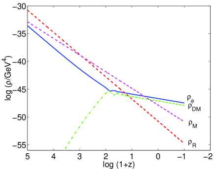
Figure 7: The late time evolution of the energy densities of the scalar field $\rho_{\phi}$, dark matter $\rho_{\rm DM}$, baryons $\rho_{M}$ and radiation $\rho_{\gamma}$, in the coupled quintessence model when all of the dark matter is coupled to the scalar field.

We see that at early times the field scales like radiation (as $p_{\rm rad}=\rho_{\rm rad}/3$ and hence the right hand side of Eqs. (2.35) and (2.36) vanishes), and it scales like ordinary matter after the radiation-matter transition. At this stage one can take $C$ to be effectively zero in Eqs. (2.35) and (2.36) following the assumption that the $\phi$ couples to baryons very weakly. Only when the dark matter contribution becomes important, does the scalar field reach the attractor solution (1) above, driving the universe to an accelerated expansion with $\gamma_{\phi}$ very close to zero, in good agreement with observations. However, the dark matter should play an important role in the process of structure formation, which would not be possible if it becomes dominant at such a late stage. For this scenario to be viable we are forced to introduce a component of dark matter that is coupled to the scalar field and a component that is not. An alternative approach, Ref. Amendola:2000uh , would be to postulate a non-linear coupling $C=C(\phi)$.

In Fig. 8 we show the evolution of $\Delta\alpha/\alpha$ for two different values of the slope of the potential $\lambda$. The damped oscillations in the direction of small redshift reflect the fact that the solution is approaching the attractor. In Fig. 9 we show the dependence of the coupling $\zeta$ on the slope of the potential $\lambda$ assuming different present contributions of the dark matter component coupled to the scalar field. The value of $C$ can be extracted from Eq. (2.37) where now we also have to take into account bi-component dark matter. Therefore,

$$C=\lambda-\frac{\lambda-\sqrt{\lambda^{2}-12\tilde{\Omega}_{c{\rm DM}}}}{2\tilde{\Omega}_{c{\rm DM}}}\,,$$ (2.42)

is a good estimate for the value of the coupling in the tracker regime. Here $\tilde{\Omega}_{c{\rm DM}}=\Omega_{c\rm DM}/(\Omega_{c\rm DM}+\Omega_{\phi})$ and $\Omega_{c{\rm DM}}$ stands for the density parameter of the dark matter component coupled to the scalar field,

We assume that $\Omega_{\phi}\approx 0.7$ today. Realistic models of coupled quintessence must have a small $\Omega_{c{\rm DM}}$ for successful structure formation. Consequently, we see from Fig. 9, that the equivalence principle constraints can only be satisfied for larger values of $\lambda$ as the amount of $\phi$-independent component of dark matter increases. For large values of $\lambda$ we have seen from Fig. 8 that the attractor is reached at a later stage, hence the field and necessarily $\Delta\alpha/\alpha$ oscillate heavily at low redshifts.

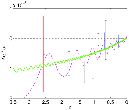
Figure 8: Evolution of $\Delta\alpha/\alpha$ for a coupled quintessence model against the observational QSO data. The coupled dark matter component has a contribution $\Omega_{c{\rm DM}}=0.05$ and $\Omega_{\phi}=0.7$ today. The solid curve corresponds to $\lambda=-100$ and the dashed curve to $\lambda=-10$.

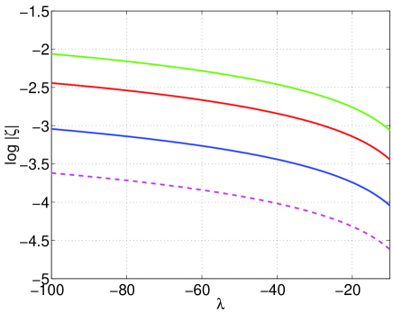
Figure 9: Dependence of $\zeta$ on the parameter $\lambda$ in the coupled quintessence model. The curves correspond to different contributions of the coupled dark. From top to bottom we have $\Omega_{c{\rm DM}}=0.02,~{}0.05,~{}0.25$, and we assume $\Omega_{\phi}=0.7$ today. The dashed curve corresponds to the variation of $\zeta$ in the uncoupled case of Sec. 2.1.

As in the case of a pure exponential potential it turns out that $\dot{\alpha}/\alpha=4.8\times 10^{-16}~{}{\rm yr}^{-1}$. However note that this is the value that corresponds to the attractor solution. Since the field is oscillating around the latter, the value of $\dot{\alpha}/\alpha$ can actually be larger by an order of magnitude or smaller, depending on the phase of oscillations.

The calculation of $\alpha$ at the time of primordial nucleosynthesis is more involved as it requires the calculation of the redshift where the attractor behaviour is reached. Our estimate for the relative change of $\alpha$ at BBN time, $\Delta\alpha/\alpha\approx 10^{-3}$, is consistent with limit (1.5).

2.5 Other quintessence models

In this subsection we analyze some other quintessence models suggested in the literature and evaluate if a coupling to the electromagnetic field can provide a realistic scenario compatible with terrestrial and cosmological observations. In Fig. 10 we plot the late time evolution of $\Delta\alpha/\alpha$ for three models, the two exponential case Barreiro:1999zs , the Albrecht-Skordis model Albrecht:1999rm , and variations to the SUGRA-inspired model proposed in Brax:1999gp . Also included in the plot are the data points of Webb et al Webb01 . In Table 1 we collect other relevant pieces of information such as typical values of the quantities $\zeta$, $\dot{\alpha}/\alpha$ and $\Delta\alpha/\alpha$ at nucleosynthesis. In addition, we indicate which models exhibit oscillatory behaviour at late times.

Model	$A$	$B$	$\zeta\times 10^{5}$	$\dot{\alpha}/\alpha\times 10^{16}$	$\Delta\alpha/\alpha(z=0.14)$	$\Delta\alpha/\alpha(z=10^{10})$	osc
2EXP a	10	–8	–20	8.6	$-3.2\times 10^{-6}$	$1.6\times 10^{-3}$	$\sqrt{}$
b	15	0.1	3.9	4.0	$-8\times 10^{-7}$	$-2.2\times 10^{-4}$	$\times$
c	10	–0.5	3.9	–0.2	$-7\times 10^{-8}$	$-3.2\times 10^{-4}$	$\sqrt{}$
A-S d	10	$0.9/A^{2}$	–50	–1.7	$2\times 10^{-6}$	$3.5\times 10^{-3}$	$\sqrt{}$
e	6	$1.1/A^{2}$	4.5	1.2	$-2\times 10^{-6}$	$-5.5\times 10^{-4}$	$\times$
f	6	$0.985/A^{2}$	11.2	–1.4	$-1\times 10^{-8}$	$-1.4\times 10^{-3}$	$\sqrt{}$
g	8.5	$0.93/A^{2}$	–30	–4.7	$-1\times 10^{-8}$	$2.5\times 10^{-3}$	$\sqrt{}$
SUGRA h	$0.5$	–11	1.08	4.4	$-9\times 10^{-7}$	$-0.3\times 10^{-4}$	$\times$
i	$0.5$	–11	–0.85	4.5	$-9\times 10^{-7}$	$-0.9\times 10^{-4}$	$\times$
j	20	–2	25	10.7	$-3\times 10^{-6}$	$4.4\times 10^{-4}$	$\sqrt{}$
k	2.2	–2	–1.7	–0.8	$-2\times 10^{-8}$	$-9\times 10^{-5}$	$\sqrt{}$

Table 1: Approximate values for $\zeta$, $\dot{\alpha}/\alpha(z=0)$ and $\Delta\alpha/\alpha$ for BBN $(z=10^{10})$ and Oklo phenomenon $(z=0.14)$ epochs for several quintessence models. 2EXP: $V=V_{0}\left(e^{A\kappa\phi}+e^{B\kappa\phi}\right)$, Ref. Barreiro:1999zs ; A-S: $V=\kappa^{-4}e^{-A\kappa\phi}\left[(\kappa\phi-C)^{2}+B)\right]$, Ref. Albrecht:1999rm ; SUGRA: $V=V_{0}\exp\left(A(\kappa\phi)^{2}\right)(\kappa\phi)^{B}$, Ref. Ng:2001hs . In the Sugra model (h) the initial condition of the field is $(\kappa\phi_{\rm in})^{2}\ll B/2A$ and in model (i) $(\kappa\phi_{\rm in})^{2}\gg B/2A$. The models which have late time oscillations of the field have a tick in the last column. We have assumed $\Omega_{\phi}=0.7$ at present.

The SUGRA model (h) in the table is the original one of Ref. Brax:1999gp , in which the field rolls along the power law slope of the potential whereas in the remaining cases the field starts rolling from the exponential side. This table suggests that various models can be consistent with the present day constraints on $\dot{\alpha}/\alpha$ and with the BBN bounds, however only a few satisfy the Oklo bound and only at the cost of severe fine tuning. The latter models are labeled with (c), (f), (g) and (k) in Table 1. In these models, the field performs a low amplitude late time oscillation hence satisfying the Oklo bound. Models (f) and (g) were recently analysed in Ref. AG . The possibility for the kind of behaviour of model (g) was pointed out before in Ref. Chiba . It is clear from Fig. 10 and Table 1 that in order to have a realistic way of constraining quintessence models we need to employ the wealth of data available on the variations of $\alpha$ over time scales much larger than those observed through the QSO observations.

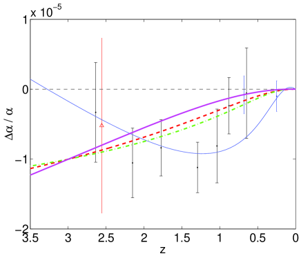
Figure 10: Late time evolution of $\Delta\alpha/\alpha$ for the models in Table 1 that pass the Oklo bound: 2EXP model (c) in dashed line; A-S models (f) and (g) of Ref. AG in light solid and solid lines respectively; SUGRA model (k) in dot-dashed line.

In the next section we propose a mechanism that enable us to reconcile a large detection of a variation on $\alpha$ at large redshift with the tight Oklo constraint without need of fine tuning in the parameters of the potential.

3 Non-minimal coupling of quintessence to the electromagnetic field

In this section, we propose a radical alternative to the allowed couplings between the quintessence and electromagnetic field, which will allow us to reconcile all the current constraints on the variation of $\alpha$ with the data. We start by asking what motivates a linear coupling between quintessence and the electromagnetic field? Obviously, there are two simple arguments for this choice: its apparent simplicity and the fact that almost any interaction can be reduced to this form if $B_{F}(\phi)$ can be expanded as a series in $\phi(z)-\phi_{0}$ provided that the latter is small. This linearization can break down for larger $\phi(z)$, and thus the comparison with $\Delta\alpha/\alpha$ at very high $z$ (i.e. BBN limits) can only tell us whether the linear dependence needs to be modified. Of course the linear choice is not the only possibility, and quadratic couplings between matter and the scalar field DP ; OP and const+$\exp{\{-\kappa\phi\}}$ couplings Damour:2002nv being also actively discussed in the past. All these approaches share the same weakness: they do not calculate these dependences from first principles but rather simply postulate them. In many ways it is analogous to simply choosing a potential for a tracker field by hand. Clearly, when an ad hoc choice of $B_{F}(\phi)$ is allowed, the profile of $\alpha(t)$ cannot be calculated and any $\alpha(t)$ is possible. In particular, one can “engineer” such a function $B_{F}(\phi)$ such that both the Oklo constraint and Webb et al. data points are satisfied. Moreover, one can choose $dB_{F}(\phi)/d\phi(z=0)\ll\kappa$, suppressing the fifth force mediated by $\phi$ DP ; Damour:2002nv .

We would like to point out another rather generic scenario where the effective fine structure constant is modified in atomic physics but has almost no impact on nuclear and particle physics. This would allow us to reconcile the Oklo constraints with the results of Webb et al. and suppress the non-universality of the gravitational force mediated by $\phi$. To do this we propose a momentum dependent modification of the interaction (LABEL:tx). Quite generically, the vertex between two photons and a $\phi$ field can be written in the momentum representation as

$$\left[-\left(p_{\mu}+\frac{1}{2}q_{\mu}\right)\left(p_{\nu}-\frac{1}{2}q_{\nu}\right)\right.\hskip 34.14322pt$$

$$+\left.g_{\mu\nu}\left(p^{2}-\frac{q^{2}}{4}\right)\right]f[p^{2},q^{2},(pq),\phi]\,,$$ (3.43)

where $p\pm q/2$ are photon momenta and $q$ is the momentum of the scalar field. Eq. (3.43) has introduced a form factor $f$ that depends on the momenta and the value of the scalar field. The minimal choice of coupling, $f[p^{2},q^{2},(pq),\phi]=\kappa\zeta$, was discussed in previous sections. For all practical purposes, one can neglect the momentum of the scalar field so that

$$f[p^{2},q^{2},(pq)]=f[p^{2}]\,.$$ (3.44)

Let us now imagine that this coupling has a form factor which tends to zero as $p^{2}$ becomes larger than a certain critical momentum scale $\mu$. For definiteness, we assume a power-like suppression,

$$f[p^{2}]=\kappa\tilde{\zeta}\frac{\mu^{2}}{\mu^{2}-p^{2}}\,,$$ (3.45)

where $\tilde{\zeta}$ is the momentum independent fundamental constant. This choice of $f$ leads to the anomalous dependence of the effective coupling constant on the photon virtuality such that

$$\alpha(p^{2})=\alpha_{c}(1+\kappa\zeta_{\rm eff}\phi)\hskip 9.95863pt{\rm with}$$

$$\zeta_{\rm eff}(p^{2})=\tilde{\zeta}~{}\frac{\mu^{2}}{\mu^{2}-p^{2}}=\left\{\begin{array}[]{ll}\tilde{\zeta}\hskip 15.6491pt{\rm for}\,\,|p^{2}|\ll\mu^{2}\\ 0\hskip 15.6491pt{\rm for}\,\,|p^{2}|\gg\mu^{2}\end{array}\right.\,.$$ (3.48)

In other words, the high virtuality photons always couple to matter with a constant time-independent strength $\alpha_{c}$, while the couplings of low virtuality photons are modified by the presence of $\phi$ which evolves with cosmological time. Of course, $\alpha_{c}$ will have a usual high-energy log-type running with the momentum. In the language of operators the choice (3.45) would correspond to a new non-local operator that can be written as

$${\cal L}_{\phi F}=-\frac{1}{4}F_{\mu\nu}F^{\mu\nu}-{1\over 4}\tilde{\zeta}\kappa\phi F_{\mu\nu}\frac{\mu^{2}}{\mu^{2}+\partial^{2}}F^{\mu\nu}\,.$$ (3.49)

The zeroth order term in the expansion over $\partial^{2}/\mu^{2}$ corresponds to a usual linearized form of (2.13) that we were using in the previous sections. We also note that Eq. (3.49) does not allow for arbitrary additive redifinition of $\phi$ at $z=0$. As before, we assume that the cosmological evolution of $\phi$ is driven by its self potential.

In the absence of the form factor, the effective coupling between nucleons and scalar field, $\zeta_{N}\kappa\phi\bar{N}N$ (see the notations of Ref. OP ), induced via the coupling to photons is given by $\zeta_{N}\sim 10^{-3}\zeta<10^{-6}$ GL , leading to the bound (1.7). It is clear that in order to obtain a further suppression of $\zeta_{N}$ coupling by the form factor (3.45) one should choose the scale $\mu$ to be lower than the characteristic virtualities of photons involved in the hadronic and nuclear matrix elements. The latter are of the order of the inverse characteristic size of a system, which in the case of $\zeta_{N}$ coupling is the size of the nucleon. For example, the coupling of $\phi$ to nucleons, $\zeta_{N}$, will receive a typical suppression of $\mu^{2}/(200~{}{\rm MeV})^{2}$ for $\mu\mathrel{\raise 1.29167pt\hbox{$<$\kern-7.5pt\lower 4.30554pt\hbox{$\sim$}}}200~{}{\rm MeV}$:

$$\zeta_{N}\sim 10^{-3}\tilde{\zeta}\frac{\mu^{2}}{(200~{}{\rm MeV})^{2}},$$ (3.50)

where $200~{}{\rm MeV}$ is roughly the inverse size of a nucleon. This suppression can be even stronger for a steeper form factor. This leads to a considerable weakening of all constraints coming from the non-universality due to the $\phi$-exchange. For example, choosing $\mu$ around $10$ MeV, we get an additional $10^{-3}-10^{-2}$ suppression so that the effective coupling to nucleons is now much smaller $\zeta_{N}\sim(10^{-6}-10^{-5})\tilde{\zeta}$. This results in a much weaker, $\tilde{\zeta}\mathrel{\raise 1.29167pt\hbox{$<$\kern-7.5pt\lower 4.30554pt\hbox{$\sim$}}}1$, bound than eq. (1.7).

Likewise, the bounds coming from Oklo phenomenon will also be weakened. This is because in the presence of the form factor (3.48) the dependence of nuclear levels on $\phi$ entering in the standard calculation DP ; Fujii ; OPQ is suppressed and consequently these levels are less affected by the change in the $\phi$ field. Indeed, the expected weakening of the Oklo bound is at least a factor of $\mu^{2}/(50~{}{\rm MeV})^{2}\sim 0.04$ with the same choice of $\mu$. Here $50$ MeV is a typical inverse radius of a heavy nucleus. This is just enough to make the results of Oklo analysis DP ; Fujii ; OPQ compatible with Webb et al. even with $\dot{\alpha}\simeq$ const and without any fine tuning.

On the other hand, the atomic physics phenomena for which the characteristic photon virtualities are much smaller than $\mu\sim 10$ MeV will be sensitive to “dressed” $\alpha$ that evolves as a function of $\phi$. In particular, this refers to the relativistic corrections to the atomic energy levels, used for the QSO analysis of Webb et al. Thus, the existence of the form factor allows to “isolate” the phenomenon of changing alpha to atomic physics and remove it from nuclear and particle physics.

The anomalous dependence of the fine structure constant on the photon momentum (3.48) can be probed with high precision QED measurements, as different experiments probe different photon virtualities. Some of these measurements are performed with atomic and condensed matter systems, where the characteristic momentum transfers are much smaller than $\mu$. Take, for example, the determination of $\alpha$ from the quantum Hall effect where the characteristic momenta of photons are very small. This experiment will be sensitive to the “dressed” value of $\alpha(p^{2}\simeq 0)$ with obvious condition $\phi=\phi(z=0)$. On the other hand, the precision measurements sensitive to QED radiative corrections such as electron and muon anomalous magnetic moments can also probe $\alpha$ at virtualites comparable to $\mu$ where the value of $\alpha$ is given by (3.48). The expression for the magnetic dipole moment of the electron and muon including the first loop correction will be given by

$$d_{i}\simeq\frac{e(p^{2}\simeq 0)}{m_{i}}\left[1+\frac{\alpha(p^{2}\simeq m_{i}^{2})}{2\pi}\right]\,,$$ (3.51)

where $i=e,\mu$. The electron $g-2$ experiment g-2e has measured the anomalous magnetic moment of the electron to an accuracy that allows for the extraction of $1/\alpha$ to nine digits. Now we have to take into account that the one-loop correction has some photons with virtualities $p^{2}\simeq\mu^{2}\sim(10~{}{\rm MeV})^{2}$. This will introduce a correction to $g-2$ of the electron due to the anomalous behaviour of $\alpha$ at large momenta at the level of

$$\Delta(g-2)_{e} \sim \tilde{\zeta}\kappa\phi\left(\frac{\alpha}{2\pi}\right)\left(\frac{m_{e}^{2}}{\mu^{2}}\right)$$ (3.52)

$$\sim 10^{-10}-10^{-11}\,,$$

for $\mu\sim 10$ MeV and typical $\tilde{\zeta}\kappa\phi\sim 10^{-5}$ suggested by Webb et al. results. This correction is taken relative to the value of $g-2$ calculated with “fully dressed” value of $\alpha$ (3.48). Since $(g-2)_{e}$ is used for the extraction of $\alpha$, one should absorb correction (3.52) into the measured value of $\alpha$ and compare it with the second best determination of the fine structure constant from the quantum Hall effect. The correction (3.52) corresponds to the shift of $1/\alpha$ in the eighth digit which appears to be marginally consistent with the determination of $\alpha$ from the solid state physics Mohr:2000ie .

The largest effect is expected in the $g-2$ of the muon, where the radiative corrections probe “undressed” $\alpha$, or $\alpha_{c}$, (3.48) at virtualities comparable to the muon mass, which is much larger than a chosen value of $\mu\simeq 10$ MeV. Therefore, the expected correction to the muon anomalous magnetic moment (relative to the value one would expect with “dressed” $\alpha$ given by (3.48)) will be on the order

$$\Delta(g-2)_{\mu}\sim\tilde{\zeta}\kappa\phi\left(\frac{\alpha}{2\pi}\right),$$ (3.53)

which is larger than both the experimental and theoretical accuracy of $(g-2)_{\mu}$, unless $\tilde{\zeta}\kappa\phi<10^{-6}$, where $\phi$ is the value of the scalar field now. This might still be marginally consistent with Ref. Webb01 if $\tilde{\zeta}\kappa\phi(z\simeq 0.5)\sim 10^{-5}$.

Therefore, the anomalous running of $\alpha$ with the momentum (3.48), (3.48) comes tantalizingly close to the accuracy of modern tests of QED. At the same time, it allows us to disconnect the phenomenon of “changing $\alpha$” from nuclear and hadronic physics. This way the results of Webb et al. coming from the atomic physics, are not in contradiction with Oklo phenomenon and are of no immediate consequence for the fifth-force experiments.

4 Conclusions

We have studied a variety of cosmological scalar field models coupled to the electromagnetic Lagrangian. The evolution of the scalar field over cosmological times induces the effective change of the fine structure constant. We have considered two generic possibilities:

(i) Tracker solution. We have shown that for a wide range of models where the scalar field is tracking, there exists a region in parameter space which allows concordance with the QSO data on non-zero $\Delta\alpha/\alpha$ Webb01 with other constraints on $\Delta\alpha/\alpha$ coming from the Big Bang nucleosynthesis as well as the precision measurements of the universality of the gravitational force. The predictions for the present day $\dot{\alpha}/\alpha$ are typically within one order of magnitude from current experiments and within the reach of near future laboratory experiments. Typical constraints on the parameter space are shown in Figs. 1 and 4. There is an upper bound on the mass scale $M$ or $V_{0}$ from the requirement that the tracking solution persists until $z=0$ and $\rho_{\phi}\ll\rho_{B}$ today. The consequence of this is the lower bound on $\zeta$, the coupling between the scalar field and the electromagnetic $F_{\mu\nu}F^{\mu\nu}$. This typically leads to $\zeta>10^{-5}$ (see Figs. 1, 4 and from the dashed line in Fig. 9) in the region of parameters studied. The universality of the gravitational force puts an upper bound on the coupling, $\zeta<10^{-3}$.

(ii) Dark energy. We have found that the simple inverse power law model for quintessence also offers a small region of parameter space in agreement with the QSO observations. Here, for a chosen $n$ the mass scale $M$ is fixed, therefore, the only free parameter remaining is the coupling $\zeta$. To fit the QSO data for a chosen $n$ we obtain one single $\zeta$ (or a small window due to the uncertainties related with the data). We have also considered the model of the scalar field coupled to the dark matter. We have found that only large values (if $\lambda$ is negative) of the slope of the scalar potential allow this model to pass the equivalence principle constraints. This model can generate oscillatory behaviour for $\alpha(z)$ which may lead to the enhancement of the present day signal of $\dot{\alpha}/\alpha$. We looked at other models of quintessence suggested in the literature. Their relevant properties for this work are summarised in Table 1. We expect that complimentary information on the present equation of state of the universe, on the coupling $\zeta$ and on the ratio $\dot{\alpha}/\alpha$ can help us to back up or rule out models of quintessence and scenarios in which a dynamical subdominant scalar field is evolving in a tracking regime.

A notable feature of this detailed analysis is that apart from a small region of parameter space in some quintessence models with late time oscillations (e.g., models (c), (f), (g) and (k) of Table 1) we have not come accross a model that satisfies both the Oklo bound $|\Delta\alpha/\alpha|\mathrel{\raise 1.29167pt\hbox{$<$\kern-7.5pt\lower 4.30554pt\hbox{$\sim$}}}10^{-7}$ at $z\sim 0.14$ and $\Delta\alpha/\alpha\sim-10^{-5}$ at $z\sim 1$ reported by Webb et al.. In an attempt to reconcile this, we have suggested that the existence of form factor in the coupling of $\zeta$ at around 10 MeV with respect to the photon momentum may lead to the suppression of the effective coupling between $\phi$ and nucleons and nuclei. This is sufficient to isolate the phenomenon of changing couplings to the realm of atomic physics, while relaxing the bounds coming from the Oklo phenomenon and the fifth-force experiments. This amounts to postulating an anomalous running of $\alpha$ with momentum and thus gives an additional possibility of checking this idea with high-precision QED measurments, sensitive to various ranges of the photon virtualities.