Semileptonic Hyperon Decays

Abstract

We review the status of hyperon semileptonic decays. The central issue is the $V_{us}$ element of the CKM matrix, where we obtain $V_{us}=0.2250(27)$. This value is of similar precision, but higher, than the one derived from $K_{l3}$, and in better agreement with the unitarity requirement, $|V_{ud}|^{2}+|V_{us}|^{2}+|V_{ub}|^{2}=1$. We find that the Cabibbo model gives an excellent fit of the existing form factor data on baryon beta decays ($\chi^{2}=2.96$ for 3 degrees of freedom) with $F+D=1.2670\,\pm 0.0030$, $F-D=-0.341\pm 0.016$, and no indication of flavour $SU(3)\,$breaking effects. We indicate the need of more experimental and theoretical work, both on hyperon beta decays and on $K_{l3}$ decays.

1 Introduction

It is nearly forty years since Cabibbo proposed a model cab for weak hadronic currents based on $SU(3)$  symmetry. This model led to detailed predictions for the beta decays of the baryon octet, in particular for the beta decays of hyperons. It has taken nearly four decades to test this model experimentally. The model is now embedded in the standard model of quarks and leptons and their interactions, and its principles are most conveniently illustrated in terms of the quark triplet $u,d,s$. The $d\rightarrow u,\,s\rightarrow u$ and lepton matrix elements of the weak current are in the ratio of $\cos{\theta_{C}}:\sin{\theta_{C}}:1$. The Lorentz structure of the current is $V-A$, vector-minus-axial-vector, and $\theta_{C}$ — the Cabibbo angle — is a parameter to be determined from experimental data.

The generalization of Cabibbo universality to three generations of quarks was given by Kobyashi and Maksawa km with a weak current with the flavour structure $\sum_{ik}\bar{u}_{i}V_{ik}d_{k}$, where $u_{i}=\{u\,c\,t\}$ are the $Q=2e/3$ quarks, and $d_{k}=\{d\,s\,b\}$ the $Q=-e/3$ quarks. They observed that this extension could accomodate $CP$ violation. The $3\times 3$ matrix $V$ is known as the Cabibbo-Kobyashi-Maksawa (CKM) matrix, and $V_{ud}\approx\cos\theta_{C},V_{us}\approx\sin\theta_{C}$.

Quark beta decay is not accessible to experiment and we must rely on the next best available cases, the meson octet or the baryon octet. In this article we will concentrate on the study of the beta decays in the baryon octet, which include both strangeness-conserving decays and strangeness-changing decays. Among the first we find ordinary nuclear beta decay, in particular the beta decay of free neutrons, but also the $\Sigma\rightarrow\Lambda$ beta decays. Strangeness violating decays include $\Lambda\rightarrow p,\;\Sigma^{-}\rightarrow n,\;\Xi^{-}\rightarrow\Lambda,\;\Xi^{-}\rightarrow\Sigma^{0}$ and $\Xi^{0}\rightarrow\Sigma^{+}$ beta decays.

If one neglects $SU(3)$  breaking effects, the ensemble of baryon beta decays is described by three parameters, $\theta_{C}$ and the $F$ and $D$ parameters for the axial-vector matrix elements. The second parameter arises because there are two irreducible matrix elements for an octet current between two octets. It was left to experiments to find how well the data from all decays in the baryon octet are described by these two parameters. As is frequently the case in testing a fundamental theory, the experimental tests proved to be highly non-trivial. One encounters both theoretical and experimental difficulties.

On the experimental side, the beta-decay branching ratios of hyperons are typically 1/1000 or less, requiring considerable skill and resources to separate the beta decays from dominant two-body decay backgrounds. The notable exception is the neutral cascade $\Xi^{0}\rightarrow\Sigma^{+}\,e^{-}\,\bar{\nu}$ decay, which is easily distinguished from $\Xi^{0}\rightarrow\Lambda\pi^{0}$, the only two body decay that is energetically allowed.

If one seeks a precision test of the theory, one has to disentangle the effects of forbidden contributions to hyperon decays, such as the weak magnetism form factor, from those arising from the allowed contributions. Considerable skill and resources, in this case polarized hyperon beams, are required to disentangle the individual form factor contributions. Thus, from the lowest lying hyperon (lambda) to the highest (cascade), the experiments have, at each stage, challenged state-of-the-art-techniques.

Only now, with the recent measurement of $\Xi^{0}$ beta decay cb ; ffcb can we form a perspective of how well the model actually accounts for the data. As we shall see, it accounts for them extremely well.

On the theoretical side the main impediment to a model-independent test of the theory is the lack of a model-independent computation of effects arising from the breaking of $SU(3)$  symmetry — in modern terms, from the mass difference between the $s$ and the $d$ quarks. Although present data on baryon beta-decay are in excellent agreement with the predictions of unbroken $SU(3)$, a model independent evaluation of $SU(3)$-breaking effects would play a key role in a precision test of the unitarity of the CKM matrix. The means for such a test are probably available with the methods of lattice QCD simulations that have seen remarkable advances in recent years.

The weak mixing parameters $V_{us},V_{ds}$ are already today the best known entries in the CKM matrix, but an improvement would be very valuable, as it can lead to a better check on the unitarity of the $V$ matrix. The value of $V_{us}$ presented in the Particle Data Group PDG2002 is essentially derived from $K_{l3}$ decays, while results from hyperon beta decays are given an ancillary role. We are convinced that already today the value of $V_{us}$ obtained from hyperon decay is of comparable precision to the $K_{l3}$ one. Further theoretical and experimental work should in the near future improve the situation in both hyperon and $K_{l3}$ beta decays.

1.1 Historical Note

Of course, this is the picture from an early 21^st century perspective. It is not the way pieces of the puzzle unfolded. In recounting the history, one might start with L. B. Okun’s rapporteur talk OkunRochester58 at the 1958 “Rochester Conference” at CERN. Here mesons and hyperons are represented as composite states; of pions, nucleons and lambdas (the Sakata model, SakataModel ). In fact, there is even the suggestion, later dropped, that lambda and cascade hyperons might be the constituents! Universality between the vector coupling of nuclear and mu meson beta-decay is incorporated; It is recognized that the reduced strength of $\Delta S=1$ hyperon beta decays is compatible with the decay rate of $K_{l3}$ decays, hinting at a universal suppression of strangeness-changing leptonic decays.

A key clue can be found in the thesis of Feynman’s student, Sam Berman Berman . The issue was the comparison between the experimental value of the Fermi coupling constant as deduced from neutron and muon beta decay: could the slight discrepancy be accounted for by radiative corrections? Berman and Feynman discovered that radiative corrections for beta decay had the opposite sign from that needed to close the gap between beta decay and muon decay. The conclusion of the thesis was “The disagreement between experiment and theory appears to be outside the limit of experimental error and might be regarded as an indication of the lack of universality even by the strangeness conserving part of the vector interaction.”

The closest encounter with the concept of a mixing angle appeared in a footnote to the PCAC paper by M. Gell-Mann and M. Lévy, Gell-Mann:np , which comments on the possible interpretations of Berman’s discrepancy:

“Should this discrepancy be real, it would probably indicate a partial or total failure of of the conserved vector current idea. It might also mean, however, that the current is conserved but with $G/G_{V}<1$. Such a situation is consistent with universality if we consider the vector current for $\Delta S=0$ and $\Delta S=1$ together to be something like:

$$GV_{\alpha}^{(\Delta S=0)}+GV_{\alpha}^{(\Delta S=1)}=G_{\mu}\bar{p}\gamma_{\alpha}(n+\epsilon\Lambda)(1+\epsilon^{2})^{-1/2}+...$$

And likewise for the axial-vector current. If $(1+\epsilon^{2})^{-1/2}=0.97$, then $\epsilon^{2}=.06$, which is of the right order of magnitude for explaining the low rate of $\beta$ decay of the $\Lambda$ particle. There is, of course, a renormalization factor for that decay, so we cannot be sure that the low rate really fits in with such a picture.”

On reading this footnote, two questions arise: What are the missing terms in the vector current, represented by ellipsis points? Why did Gell-Mann fail to elaborate this footnote into a complete solution after discovering the $SU(3)$  symmetry? The most probable answer is that up to 1962 there was evidence for the presence of $\Delta S=-\Delta Q$ weak transitions which could not easily fit in either the Sakata model or the octet model.

One of the first published examples of a hyperon beta decay event was a $\Delta S=-\Delta Q$ event, $\Sigma^{+}\rightarrow n\,\mu^{+}\nu$ observed in emulsions AngelaBG . This event appeared in a total observed sample of $120\,\Sigma^{+}$ decays. When in 1963 the first “large statistics” studies of hyperon decays were emerging at CERN, and no new $\Delta S=-\Delta Q$ event appeared, a rough evaluation of the relevant branching ratios convinced Cabibbo that the evidence for for $\Delta S=-\Delta Q$ could be disregarded. This observation was crucial in working out the consequences of $SU(3)$  for the weak interactions, because by neglecting the possibility of $\Delta S=-\Delta Q$ one could adopt the simplest hypothesis, according to which the weak current was a member of an $SU(3)$  octet. Several years later this event and other evidence for $\Delta S=-\Delta Q$ decays was dismissed as background Cronin68 .

The present PDG limit PDG2002 , based on fairly old (pre-1975) experiments,

$$\frac{\Sigma^{+}\rightarrow n\,\ell^{+}\nu}{\Sigma^{-}\rightarrow n\,\ell^{-}\bar{\nu}}<0.043$$

could and should be substantially improved.

In 1963 Cabibbo cab proposed a theory of the weak current, parameterized by a single mixing angle $\theta_{C}$ , in the context of the octet model of $SU(3)$  symmetry. The central assumption was that the weak current $J_{\alpha}$ is a member of an octet of currents $J^{i}_{\alpha}=V^{i}_{\alpha}+A^{i}_{\alpha}$, where $V^{i}_{\alpha}$ and $A^{i}_{\alpha}$ are octets of vector and axial currents,

$$J_{\alpha}=\cos\theta_{C}(J^{1}_{\alpha}+iJ^{2}_{\alpha})+\sin\theta_{C}(J^{4}_{\alpha}+iJ^{5}_{\alpha})$$ (1)

By assuming that the vector and axial parts of the weak current are “parallel,” i.e. the same element of the respective octets, the theory included the $V-A$ hypothesis, and it also included the Conserved Vector Current (CVC ) hypothesis, by assuming that the vector part of the weak current belongs to the same octet as the electromagnetic current.

The theory led to a very detailed description of semileptonic decays of baryons and mesons in terms of a small number of parameters, leading to predictions for the matrix elements that have proven durable and remarkably accurate.

When expressed in terms of quarks, which were only proposed in 1964, the weak current of Ref. cab takes the simple form

$$J_{\alpha}=\cos\theta_{C}\,\bar{u}\gamma_{\alpha}(1+\gamma_{5})d+\sin\theta_{C}\,\bar{u}\gamma_{\alpha}(1+\gamma_{5})s$$ (2)

1.2 Intimations of $CP$ violation

Soon after Cabibbo proposed the quark mixing hypothesis, the suggestion was made gla_cab that the same picture could naturally accommodate $CP$ violation by allowing the mixing angle to be complex (adding a phase). However, it was easily seen that a $2\times 2$ unitary matrix (in the case of four quarks) can always be reduced to a form with real elements, and thus necessarily preserves $CP$.

In 1973 Kobayashi and Maskawa noted that the mixing of three quark families entails a single complex phase that cannot be eliminated by field redefinitions. They thus proposed that the four-quark model should be extended to a six-quark model in which mixing offers a natural explanation for the existence of $CP$ violation. Their proposal predated by four years the discovery of $\Upsilon$ particles, the first experimental detection of a fifth quark, the $b$ quark.

In the standard model with six quarks the network of transition amplitudes between the charge –1/3 quarks, $d,s,b$, and the charge 2/3 quarks, $u,c,t$ is described by a unitary matrix $V$, the CKM matrix, whose effects can be seen as a mixing between the $d,s,b$ quarks,

$$\begin{pmatrix}d^{\prime}\\ s^{\prime}\\ b^{\prime}\end{pmatrix}=\begin{pmatrix}V_{ud}&V_{us}&V_{ub}\\ V_{cd}&V_{cs}&V_{cb}\\ V_{td}&V_{ts}&V_{tb}\end{pmatrix}\begin{pmatrix}d\\ s\\ b\end{pmatrix}$$ (3)

The new description can be seen as an extension of the current mixing of Eq. (1), or the quark mixing in Eq. (2), the relation between the two formulations being given by

$$\tan\theta_{C}=\frac{V_{us}}{V_{ud}}.$$ (4)

The recent observation of direct $CP$ violation in the neutral kaon system KTeVepsi ; Lai:2001ki and the $CP$ violation in $B$-meson oscillations Babar ; Belle are in brilliant confirmation of this picture CabibboLP01 .

1.3 Status in 1983-4

Hyperon beta decay has an important role in the study of weak interactions, both by establishing the validity of the predicted pattern of branching ratios and form factors, and by contributing to the determination of the parameter $\sin\theta_{C}$. The first task is substantially achieved at the present level of accuracy, and has been completed with the recent results on the beta decay of the neutral cascade. The road to the present satisfactory state of affairs was not easy, and we will mention some of the difficulties which were encountered on the way.

At the time of the last Annual Review of Nuclear and Particle Science article on hyperon decays, by Gaillard and Sauvage, Gaillard:1984ny nearly twenty years ago, the key experimental tests of the Cabibbo theory had not yet been done. While it is true that lambda beta decay had been found to be approximately $V-A$ as required, the theory faced its first critical test in sigma minus beta decay. Taking the $F/D$ ratio from any two decays, say neutron and lambda, the theory required sigma minus beta decay to appear $V+A$. This surprising sign reversal was considered at the time the “go or no-go” test of the Cabibbo theory. Measuring the sign convincingly required polarized sigma minus. Low energy experiments relied on tertiary polarized sigmas from pions or kaons. The statistics were meager, the control of systematics problematic, and the results less than compelling. If anything, the $V-A$ sign appeared favored by the data Keller .

The turning point was determined by an experimental innovation, the invention and development of hyperon beams. When such beams were discovered to be significantly polarized, a new era of precision experiments with excellent control of systematics was inaugurated. With the ability to produce and reverse polarization, correlations between momenta and polarization could be measured in a precise and bias-cancelled way. New precise experiments settled the question of the $\Sigma^{-}$ beta decay in favor of the Cabibbo prediction (see Section 3.2). The high-energy hyperon beam proved to be the enabling technology for carrying out precision measurements of hyperon decay properties.

2 Theoretical Issues

In this section we discuss different issues that must be taken into account in an accurate treatment of hyperon semileptonic decays. These include the issue of the breaking of flavour $SU(3)$  symmetry, radiative corrections, and the $q^{2}$ dependence of the form factors. We will however start from a discussion of the general form of the matrix element, which we will express in terms of a convenient 2-component spinor formulation bri , and of the different observables in hyperon decays.

2.1 Baryon Matrix Elements

The $V-A$ transition matrix element for the generic hyperon beta-decay process $B\rightarrow\,b\,e^{-}\,\bar{\nu}$, where $B$ and $b$ are the initial and final-state baryons, can be written in the form

$$\mathcal{M}=\frac{G_{S}}{\sqrt{2}}\bar{u}_{b}\,(O^{V}_{\alpha}+O^{A}_{\alpha})\,u_{B}\,\bar{u}_{e}\,\gamma^{\alpha}\,(1+\gamma_{5})\,v_{\nu}$$ (5)

where

$$O^{V}_{\alpha} =f_{1}(q^{2})\gamma^{\alpha}+\frac{f_{2}(q^{2})}{M_{B}}\sigma_{\alpha\beta}q^{\beta}+\frac{f_{3}(q^{2})}{M_{B}}q_{\alpha}$$ (6)

$$O^{A}_{\alpha} =\left(g_{1}(q^{2})\gamma^{\alpha}+\frac{g_{2}(q^{2})}{M_{B}}\sigma_{\alpha\beta}q^{\beta}+\frac{g_{3}(q^{2})}{M_{B}}q_{\alpha}\right)\gamma_{5}$$ (7)

The momentum transfer is $q^{\alpha}=(p_{e}+p_{\nu})^{\alpha}=(p_{B}-p_{b})^{\alpha}$ and the coupling strength $G_{S}=G_{F}V_{us}$ for $|\Delta S|=1$ and $G_{S}=G_{F}V_{ud}$ for $\Delta S=0$, where $G_{F}$ is the Fermi coupling constant, and $V_{us},V_{ud}$ are the appropriate CKM matrix elements. We employ the metric and $\gamma$-matrix conventions of Ref. GarciaBook .

The vector and axial part of the weak current are members of two octets,

$$V^{i}_{\alpha} =\bar{q}\frac{\lambda^{i}}{2}\gamma_{\alpha}q,$$

$$A^{i}_{\alpha} =\bar{q}\frac{\lambda^{i}}{2}\gamma_{\alpha}\gamma_{5}q,$$ (8)

where $\lambda^{i}/2$ are generators of $SU(3)$  . Neglecting the mass difference between the $s$ and the $u,\,d$ quarks, an explicit breaking of flavor $SU(3)$  symmetry, the form factors for baryon beta decays are related to each other. Matrix elements of an $SU(3)$  octet operator $O_{k}$ between octet states can in fact be expressed in terms of two reduced matrix elements, $F_{O},\,D_{O}$

$$\langle B_{n}|\,O_{k}\,|B_{m}\rangle=F_{O}\,f_{knm}+D_{O}\,d_{knm}$$ (9)

where $f_{knm}$ are the structure constants of $SU(3)$  and $d_{knm}$ are defined by the anticommutation relations $\{\lambda^{k},\lambda^{n}\}=2\delta_{kn}+2d_{knm}$. If we know the value of two independent matrix elements in Eq. (9), all of them can be determined.

The vector part of the weak current and the electromagnetic current belong to the same octet, so that the matrix elements of the weak current can be predicted on the basis of the electromagnetic form factors of the proton and neutron. This is true both of $f_{1}$ and of the “weak magnetism” form factor, $f_{2}$.

The allowed contribution of the axial current derives from the $g_{1}$ form factor. The leading contribution is described by the two parameters, $F$ and $D$. We will return to the problem of the $q^{2}$ dependence of $g_{1}$.

The “weak electricity” form factor, $g_{2}$, vanishes in the limit of exact $SU(3)$, as can be seen from a very simple argument: flavor $SU(3)$  symmetry connects the axial weak current to two neutral currents, $A^{3}_{\alpha}$ and $A^{8}_{\alpha}$. Since the latter are even under charge conjugation, their matrix elements cannot contain a $g_{2}$ term, which could only arise from an odd-$\mathcal{C}$ current, a “second-class current” according to the terminology of S. Weinberg WeinbergII . It is easily seen that second class currents are excluded in the framework of the standard model.

Summing up, the expression (2) of the weak current leads, in the limit of exact flavor $SU(3)$  symmetry, to simple predictions for the complex of baryon beta decays, in terms of $\theta_{C}$ and two further parameters, $D,F$, needed to describe the axial-vector form factors in the various decays. The $D,F$ parameters are the generalization to $SU(3)$  of the reduced matrix element of the Wigner-Eckart theorem for $SU(2)$. The vector form factor $f_{1}(0)$ is directly predicted in terms of $\theta_{C}$ and the nucleon electric charges. The weak magnetism form factor $f_{2}(0)$ is predicted in terms of $\theta_{C}$ and the well-measured values of neutron and proton magnetic moments. The predictions for all of the octet baryons are given in Table 1.

Table 1: Cabibbo model predictions for octet baryon beta decays

Decay	Scale	$f_{1}(0)$	$g_{1}(0)$	$g_{1}/f_{1}$	$f_{2}/f_{1}$
$n\rightarrow pe^{-}\overline{\nu}$	$V_{ud}$	1	$D+F$	$F+D$	$\frac{M_{n}}{M_{p}}\frac{(\mu_{p}-\mu_{n})}{2}$ = 1.855
$\Xi^{-}\rightarrow\Xi^{0}e^{-}\overline{\nu}$	$V_{ud}$	-1	$D-F$	$F-D$	$\frac{M_{\Xi^{-}}}{M_{p}}\frac{(\mu_{p}+2\mu_{n})}{2}$ = -1.432
$\Sigma^{\pm}\rightarrow\Lambda e^{\pm}\nu$	$V_{ud}$	0a	$\sqrt{(}\frac{2}{3})D$	$\sqrt{(}\frac{2}{3})D$	$-\frac{M_{\Sigma^{\pm}}}{M_{p}}\sqrt{(}\frac{3}{2})\frac{(\mu_{n})}{2}$ = 1.490
$\Sigma^{-}\rightarrow\Sigma^{0}e^{-}\overline{\nu}$	$V_{ud}$	$\sqrt{(}2)$	$\sqrt{(}2)F$	$F$	$\frac{M_{\Sigma^{-}}}{M_{p}}\frac{(2\mu_{p}+\mu_{n})}{4}$ = 0.534
$\Sigma^{0}\rightarrow\Sigma^{+}e^{-}\overline{\nu}$	$V_{ud}$	$\sqrt{(}2)$	$-\sqrt{(}2)F$	$-F$	$\frac{M_{\Sigma^{0}}}{M_{p}}\frac{(2\mu_{p}+\mu_{n})}{4}$ = 0.531
$\Xi^{0}\rightarrow\Sigma^{+}e^{-}\overline{\nu}$	$V_{us}$	1	$D+F$	$F+D$	$\frac{M_{\Xi^{0}}}{M_{p}}\frac{(\mu_{p}-\mu_{n})}{2}$ = 2.597
$\Xi^{-}\rightarrow\Sigma^{0}e^{-}\overline{\nu}$	$V_{us}$	$\frac{1}{\sqrt{(}2)}$	$\frac{1}{\sqrt{(}2)}(D+F)$	$F+D$	$\frac{M_{\Xi^{-}}}{M_{p}}\frac{(\mu_{p}-\mu_{n})}{2}$ = 2.609
$\Sigma^{-}\rightarrow ne^{-}\overline{\nu}$	$V_{us}$	-1	$D-F$	$F-D$	$\frac{M_{\Sigma^{-}}}{M_{p}}\frac{(\mu_{p}+2\mu_{n})}{2}$ = -1.297
$\Sigma^{0}\rightarrow pe^{-}\overline{\nu}$	$V_{us}$	$\frac{-1}{\sqrt{(}2)}$	$\frac{1}{\sqrt{(}2)}(D-F)$	$F-D$	$\frac{M_{\Sigma^{0}}}{M_{p}}\frac{(\mu_{p}+2\mu_{n})}{2}$ = -1.292
$\Lambda\rightarrow pe^{-}\overline{\nu}$	$V_{us}$	-$\sqrt{(}\frac{3}{2})$	$-\frac{1}{\sqrt{(}6)}(D+3F)$	$F+\frac{D}{3}$	$\frac{M_{\Lambda}}{M_{p}}\frac{\mu_{p}}{2}$ = 1.066
$\Xi^{-}\rightarrow\Lambda e^{-}\overline{\nu}$	$V_{us}$	$\sqrt{(}\frac{3}{2})$	$-\frac{1}{\sqrt{(}6)}(D-3F)$	$F-\frac{D}{3}$	$-\frac{M_{\Xi^{-}}}{M_{p}}\frac{(\mu_{p}+\mu_{n})}{2}$ = 0.085
aSince $f_{1}(0)=0$ for $\Sigma^{\pm}\rightarrow\Lambda e^{\pm}\nu$, predictions are given for $f_{2}$ and $g_{1}$ rather than
$f_{2}/f_{1}$ and $g_{1}/f_{1}$.
Here $\mu_{p}=1.7928$, $\mu_{n}=-1.9130$, and $g_{2}=0$ for all decays.

2.2 The Effective Hamiltonian

The beta decay matrix element for hyperon decay can be displayed in a form that is particularly accessible for analysis of experiments. This is because there are two small parameters; $q/M$, where $q$ is the momentum transfer and $M$ a baryon mass, and $m_{e}/M$, where $m_{e}$ is the electron mass. Retaining terms up to second order in $q/M$ is sufficiently accurate for analysis of current data as well as for the foreseeable future. Terms of order $m_{e}/M$ can be safely neglected for hyperon decays, so that we can omit the scalar and pseudoscalar form factors $f_{3},g_{3}$. Hyperon muonic decays, where these form factors are relevant, have very small branching ratios and can be omitted from any precision study of the quark mixing parameters. The matrix element can be written in an effective two-component form, Ref. bri , a technique first introduced by Primakoff pri1 ; pri2 in the context of muon capture. We can then define an effective Hamiltonian for the decay $B\rightarrow be\bar{\nu}$, so that

$${\mathcal{M}}=\langle be\mid{\mathcal{H}_{\mbox{eff}}}\mid B\nu\rangle$$ (10)

with

$${\mathcal{H}_{\mbox{eff}}} = \sqrt{2}G_{S}\>\frac{1-{\vec{\mathbf{\sigma}_{\ell}}}\cdot\hat{e}}{2}\,\bigg{[}G_{V}+G_{A}{\vec{\mathbf{\sigma}_{\ell}}}\cdot{\vec{\mathbf{\sigma}_{b}}}$$ (11)

$$+G_{P}^{e}{\vec{\mathbf{\sigma}_{b}}}\cdot\hat{e}+G_{P}^{\nu}{\vec{\mathbf{\sigma}_{b}}}\cdot\hat{\nu}\bigg{]}\,\frac{1-{\vec{\mathbf{\sigma}_{\ell}}}\cdot\hat{\nu}}{2}.$$

Here $\hat{e}$ and $\hat{\nu}$ are unit vectors along the electron and antineutrino directions, while $e$, $\nu$, and $E_{B}$ are the energies of the electron, antineutrino, and initial baryon. The spin operators ${\vec{\mathbf{\sigma}_{\ell}}}$ and ${\vec{\mathbf{\sigma}_{b}}}$ act respectively on the two-component lepton and final state baryon spinors.

The effective coupling coefficients in Equation 11, $G_{V}$, $G_{A}$, $G_{P}^{e}$, and $G_{P}^{\nu}$ are functions of the form factors, but depend also on the frame of reference. The rest frames of the initial baryon $B$ and of the final baryon $b$ are of particular interest in analyzing a beta decay experiment. The rest frame of the initial baryon is particularly convenient in analyzing the decay of polarized baryons, and in this frame we have

$$G_{V} = f_{1}-\delta f_{2}-\frac{\nu+e}{2M_{B}}(f_{1}+\Delta f_{2}),$$

$$G_{A} = -g_{1}+\delta g_{2}+\frac{\nu-e}{2M_{B}}(f_{1}+\Delta f_{2}),$$

$$G_{P}^{e} = \frac{e}{2M_{B}}\left[-(f_{1}+\Delta f_{2})+g_{1}+\Delta g_{2}\right],$$

$$G_{P}^{\nu} = \frac{\nu}{2M_{B}}(f_{1}+\Delta f_{2}+g_{1}+\Delta g_{2}),$$ (12)

In the rest frame of the final-state baryon, particularly convenient if its polarization is an observable, the effective couplings are given by

$$G_{V} = f_{1}+\delta f_{2}-\frac{\nu+e}{2M_{B}}(f_{1}+\Delta f_{2}),$$

$$G_{A} = -g_{1}+\delta g_{2}+\frac{\nu-e}{2M_{B}}(f_{1}+\Delta f_{2}),$$

$$G_{P}^{e} = \frac{e}{2M_{B}}\left[-(f_{1}+\Delta f_{2})-g_{1}+\Delta g_{2}\right],$$

$$G_{P}^{\nu} = \frac{\nu}{2M_{B}}(f_{1}+\Delta f_{2}-g_{1}+\Delta g_{2}),$$ (13)

In either case $\delta=(M_{B}-M_{b})/M_{B}$ and $\Delta=(M_{B}+M_{b})/M_{B}=2-\delta$.

2.3 Decay Distributions

We give the distributions to second order in the parameter $\delta$, which is sufficient for the accuracy of experiments. Of course, to this order one must also take the $q^{2}$ dependence of the form factors into account, as will be discussed later. As noted above, we will distinguish two cases:

1. The energy spectrum and angular distribution of the leptons is studied with respect to the polarization of the initial baryon. This case will be analyzed in the rest frame of the decaying baryon, with the effective form factors given by Eq. (12).

2. The energy spectrum and angular distribution of the leptons is studied together with the polarization of the final state baryon. This case will be analyzed in the rest frame of the emitted baryon, with the effective form factors given by Eq. (13).

Let us start with the first case, where we work in the rest frame of the decaying baryon, which has a polarization $\mathbf{P}_{B}$, and we do not measure the polarization of the final state particles.

The differential decay rate is

$$d\Gamma=\frac{|\mathcal{M}|^{2}}{(2\pi)^{5}}\frac{E_{b}+M_{b}}{2M_{B}}\frac{e^{2}\nu^{3}}{(e^{\textrm{max}}-e)}de\,d\Omega_{e}\,d\Omega_{\nu}$$ (14)

After summing over final spins and averaging over the initial spin, $|M|^{2}$ is given by:

$$\mid{\mathcal{M}}\mid^{2} = G_{S}^{2}\,\xi\,\,\big{[}1+a\hat{e}\cdot\hat{\nu}+\textsf{A}\mathbf{P}_{B}\cdot\hat{e}+\textsf{B}\mathbf{P}_{B}\cdot\hat{\nu}$$ (15)

$$+\textsf{A}^{\prime}(\mathbf{P}_{B}\cdot\hat{e})(\hat{e}\cdot\hat{\nu})+\textsf{B}^{\prime}(\mathbf{P}_{B}\cdot\hat{\nu})(\hat{e}\cdot\hat{\nu})+\textsf{D}\mathbf{P}_{B}\cdot(\hat{e}\times\hat{\nu})\big{]}$$

where $\mathbf{P}_{B}$ is the polarization vector of the decaying baryon, and the different coefficients can be expressed in terms of the form factors of Eq. (12) according to

$$\xi= \mid\!G_{V}\!\mid^{2}+3\mid\!G_{A}\!\mid^{2}-2\textrm{Re}\left[G_{A}^{*}(G_{P}^{e}+G_{P}^{\nu})\right]+\mid\!G_{P}^{e}\!\mid^{2}+\mid\!G_{P}^{\nu}\!\mid^{2},$$

$$\xi a= \mid\!G_{V}\!\mid^{2}-\mid\!G_{A}\!\mid^{2}-2\textrm{Re}\left[G_{A}^{*}(G_{P}^{e}+G_{P}^{\nu})\right]$$

$$+\mid\!G_{P}^{e}\!\mid^{2}+\mid\!G_{P}^{\nu}\!\mid^{2}+2\textrm{Re}(G_{P}^{e*}G_{P}^{\nu})(1+\hat{e}\cdot\hat{\nu}),$$

$$\xi\textsf{A}= -2\textrm{Re}(G_{V}^{*}G_{A})-2\mid\!G_{A}\!\mid^{2}+2\textrm{Re}(G_{V}^{*}G_{P}^{e}+G_{A}^{*}G_{P}^{\nu}),$$

$$\xi\textsf{B}= -2\textrm{Re}(G_{V}^{*}G_{A})+2\mid\!G_{A}\!\mid^{2}+2\textrm{Re}(G_{V}^{*}G_{P}^{\nu}-G_{A}^{*}G_{P}^{e}),$$

$$\xi\textsf{A}^{\prime}= 2\textrm{Re}(G_{P}^{e*}(G_{V}+G_{A})),$$

$$\xi\textsf{B}^{\prime}= 2\textrm{Re}(G_{P}^{\nu*}(G_{V}-G_{A})),$$

$$\xi\textsf{D}= 2\textrm{Im}(G_{V}^{*}G_{A})+2\textrm{Im}(G_{P}^{e}G_{P}^{\nu*})(1+\hat{e}\cdot\hat{\nu})+2\textrm{Im}\left[G_{A}^{*}(G_{P}^{\nu}-G_{P}^{e})\right].$$ (16)

We next consider the case where the energy spectrum and angular distribution of the leptons is studied with respect to the polarization of the final-state baryon, $\mathbf{P}_{b}$. Electron and antineutrino spins are again not observed; however, this case focuses on measurement of the final baryon polarization. The invariant matrix element is in this case given by

$$\mid{\mathcal{M}}\mid^{2} = G_{S}^{2}\,\xi\,\,\big{[}1+a\hat{e}\cdot\hat{\nu}+\textsf{A}\mathbf{P}_{b}\cdot\hat{e}+\textsf{B}\mathbf{P}_{b}\cdot\hat{\nu}$$ (17)

$$+\textsf{A}^{\prime}(\mathbf{P}_{b}\cdot\hat{e})(\hat{e}\cdot\hat{\nu})+\textsf{B}^{\prime}(\mathbf{P}_{b}\cdot\hat{\nu})(\hat{e}\cdot\hat{\nu})+\textsf{D}\mathbf{P}_{b}\cdot(\hat{e}\times\hat{\nu})\big{]}$$

and the different coefficients are given by

$$\xi= \mid\!G_{V}\!\mid^{2}+3\mid\!G_{A}\!\mid^{2}-2\textrm{Re}\left[G_{A}^{*}(G_{P}^{e}+G_{P}^{\nu})\right]+\mid\!G_{P}^{e}\!\mid^{2}+\mid\!G_{P}^{\nu}\!\mid^{2},$$

$$\xi a= \mid\!G_{V}\!\mid^{2}-\mid\!G_{A}\!\mid^{2}-2\textrm{Re}\left[G_{A}^{*}(G_{P}^{e}+G_{P}^{\nu})\right]$$

$$+\mid\!G_{P}^{e}\!\mid^{2}+\mid\!G_{P}^{\nu}\!\mid^{2}+2\textrm{Re}(G_{P}^{e*}G_{P}^{\nu})(1+\hat{e}\cdot\hat{\nu}),$$

$$\xi\textsf{A}= -2\textrm{Re}(G_{V}^{*}G_{A})+2\mid\!G_{A}\!\mid^{2}+2\textrm{Re}(G_{V}^{*}G_{P}^{e}-G_{A}^{*}G_{P}^{\nu}),$$

$$\xi\textsf{B}= -2\textrm{Re}(G_{V}^{*}G_{A})-2\mid\!G_{A}\!\mid^{2}+2\textrm{Re}(G_{V}^{*}G_{P}^{\nu}+G_{A}^{*}G_{P}^{e}),$$

$$\xi\textsf{A}^{\prime}= 2\textrm{Re}(G_{P}^{e*}(G_{V}-G_{A})),$$

$$\xi\textsf{B}^{\prime}= 2\textrm{Re}(G_{P}^{\nu*}(G_{V}+G_{A})),$$

$$\xi\textsf{D}= 2\textrm{Im}(G_{V}^{*}G_{A})+2\textrm{Im}(G_{P}^{e*}G_{P}^{\nu})(1+\hat{e}\cdot\hat{\nu})+2\textrm{Im}\left[G_{A}^{*}(G_{P}^{e}-G_{P}^{\nu})\right].$$ (18)

The polarization of the final baryon may be expressed explicitly as:

$$\mathbf{P}_{b}=\frac{(\textsf{A}+\textsf{A}^{\prime}\hat{e}\cdot\hat{\nu})\hat{e}+(\textsf{B}+\textsf{B}^{\prime}\hat{e}\cdot\hat{\nu})\hat{\nu}+\textsf{D}\hat{e}\times\hat{\nu}}{1+a\hat{e}\cdot\hat{\nu}}.$$ (19)

The components of this polarization can readily be measured when the outgoing baryon $b$ is a hyperon which undergoes a subsequent weak decay $b\rightarrow b^{\prime}\pi$ with a nonzero decay asymmetry parameter $\alpha_{b^{\prime}}$. The distribution of the $b^{\prime}$ direction relative to any axis defined by a unit vector $\hat{i}$ is given by

$$\frac{1}{\Gamma}\;\frac{d\Gamma}{d\Omega_{b^{\prime}}}=\frac{1}{4\pi}(1+{\mathsf{S}_{i}}\alpha_{b^{\prime}}\,\hat{i}\cdot\hat{b^{\prime}}),$$ (20)

where ${\mathsf{S}_{i}}=\langle{\mathbf{P}_{b}}\cdot\hat{i}\rangle$ is the average polarization of $b$ in the $\hat{i}$ direction. Conceptually, it is advantageous to employ the orthonormal basis

$$\hat{\alpha} = \frac{\hat{e}+\hat{\nu}}{\sqrt{2(1+\hat{e}\cdot\hat{\nu})}},$$

$$\hat{\beta} = \frac{\hat{e}-\hat{\nu}}{\sqrt{2(1-\hat{e}\cdot\hat{\nu})}},$$

$$\hat{\gamma} = \hat{\alpha}\times\hat{\beta}.$$ (21)

Experimentally, it may be more advantageous to determine the polarization components along one or more of the outgoing particle directions ($\hat{e},\hat{\nu},\hat{b}$).

Analytic expressions for the integrated final state polarization $\textsf{S}_{e}$, $\textsf{S}_{\nu}$,$\textsf{S}_{\alpha}$,$\textsf{S}_{\beta}$ are given in Appendix A up to (and including) second order in $\delta$. We observe that $\textsf{S}_{\alpha}$ depends solely on $V\times A$ terms, while $\textsf{S}_{\beta}$ depends solely on $V\times V$ and $A\times A$ terms in conformity with Weinberg’s theorem Weinbergthm . Another useful symmetry relation is that $\textsf{S}_{e}$ and $\textsf{S}_{\nu}$ are the same as those for a polarized initial baryon (hyperon) in the zero recoil ($\delta$ $=$ 0) limit. Stated another way, the lepton correlations with respect to $\mathbf{P}_{B}$, the polarization of the initial state baryon, are related to the correlations with respect to $\mathbf{P}_{b}$, the polarization of the final state baryon by interchanging $e$ and $\nu$ throughout and reversing the sign of D.

2.4 $q^{2}$ Dependence of Form Factors

To obtain expressions which are correct to $O(q^{2})$, we can neglect the $q^{2}$ dependence of the form factors $f_{2},\,g_{2}$, whose contribution to the transition amplitude is already $O(q)$. In the limit of exact $SU(3)$  symmetry, the $q^{2}$ dependence of the vector form factor $f_{1}$ can be expressed

$$f^{bB}_{1}(q^{2}) = C^{bB}_{F}\,F_{1}(q^{2})+C^{bB}_{D}\,D_{1}(q^{2})$$

$$= C^{bB}_{F}[F_{1}(0)+\lambda_{F_{1}}\,q^{2}]+C^{bB}_{D}\,[D_{1}(0)+\lambda_{D_{1}}\,q^{2}]$$

where $C^{bB}_{F},C^{bB}_{D}$ are the appropriate $f$ and $d$ constants (Eq. 9 ), and $F_{1}(q^{2}),D_{1}(q^{2})$ the corresponding reduced form factors, that can be expressed in terms of the measured charge form factors of the proton and neutron GarciaBook , leading to

$$F_{1}(0)=1,\;D_{1}(0)=0,\;\lambda_{F}=\,6.13\,\mathrm{GeV}^{-2},\,\lambda_{D}=\,0.12\,\mathrm{GeV}^{-2}$$ (23)

The axial current form factor, $g_{1}$, can only be related to neutrino reactions, but the data are not sufficient to determine two separate slopes for the $D$ and $F$ parts. We thus follow Ref. Gaillard:1984ny and use a dipole form, e.g. in neutron beta decay case,

$$g_{1}^{np}(q^{2})=\frac{g_{1}^{np}(0)}{(1-q^{2}/M_{A}^{2})^{2}}$$ (24)

with $M_{A}=1.08\pm 0.08$ $\mathrm{GeV/c^{2}}$. A similar parametrization for the vector form factor gives

$$f_{1}^{np}(q^{2})=\frac{f_{1}^{np}(0)}{(1-q^{2}/M_{V}^{2})^{2}}$$ (25)

with $M_{V}=0.84\pm 0.04$ $\mathrm{GeV/c^{2}}$. For the $\Delta S=1$ decays, the scaling argument of Ref. Gaillard:1984ny yields $M_{V}=0.97$ $\mathrm{GeV/c^{2}}$ and $M_{A}=1.25$ $\mathrm{GeV/c^{2}}$.

2.5 Radiative corrections

Radiative corrections to beta decay have been extensively studied by A. Sirlin Sirlin and others radcor . We have already noted the central role that these played, through Berman’s work Berman , in providing an important hint of universality breaking between neutron decay and muon decay. Hyperon decay experiments are only now becoming sufficiently sensitive to require radiative corrections, and then only for a limited set of observables. A standard reference is GarciaBook .

The situation can summarized as follows:

• Integrated observables such as correlations with respect to initial or final baryon polarization or the electron–neutrino correlation are practically unaffected GarciaBook to rather high accuracy, well beyond the precision of present and contemplated experiments. For these, radiative corrections can safely be ignored.

• Decay rates and the electron spectrum are affected and need to be corrected before fitting for form factors. This applies, in particular, to the weak magnetism form factor $f_{2}$ that is sensitive to the electron spectrum. The total rate (or branching ratio) is also affected to a few percent (for example the total rate is increased by 4.4% in $\Xi^{0}\,\rightarrow\,\Sigma^{+}e^{-}\bar{\nu}_{e}$). Therefore radiative corrections must be applied to the measured beta-decay branching ratios for precise determinations of the Cabibbo angle $\theta_{C}$ .

2.6 Flavor $SU(3)$  breaking: The Ademollo-Gatto Theorem

Symmetry breaking effects can be expanded in powers of $H^{\prime}$, the $SU(3)$-breaking term in the hadron Hamiltonian. In the standard model,

$$H^{\prime}=\frac{1}{\sqrt{3}}\left(m_{s}-\frac{m_{d}+m_{u}}{2}\right)\,\bar{q}\lambda^{8}q$$ (26)

In a previous section we have considered the expansion of physical quantities in “orders of forbiddenness,” which has been standard in the beta-decay literature since Fermi’s 1934 paper. For a hyperon decay $B\rightarrow b\,e^{-}\,\bar{\nu}$, this is equivalent to an expansion in powers of $q/M_{B}$. Here we are considering a similar expansion in powers of $H^{\prime}$. Since $q\approx(M_{B}-M_{b})\approx\,H^{\prime}$, the two expansions can be combined in a single expansion in powers of the small parameter $\delta=(M_{B}-M_{b})/M_{B}$. For example, the first terms in the expansion of $f_{1}(q^{2})$ (see GarciaBook ) are

$$f_{1}(q^{2})=C^{bB}_{F}+\Delta^{1}f_{1}(0)+\Delta^{2}f_{1}(0)+q^{2}f_{1}^{\prime}(0)+\ldots,$$ (27)

where $\Delta^{1}f_{1}(0),\,\,\Delta^{2}f_{1}(0)$ are respectively the first-order and second-order $H^{\prime}$ corrections, and the omitted terms are of third order or higher in $\delta$. In the second-order expansion above we can use the exact-$SU(3)$  result in Eq. 2.4, 23 for $f_{1}^{\prime}(0)$, which appears in a second-order correction ($\propto q^{2}$).

In 1964 Ademollo and Gatto proved ad that there is no first-order correction to the vector form factor, $\Delta^{1}f_{1}(0)=0$. This is an important result: since experiments can measure $G_{S}f_{1}$, knowing the value of $f_{1}(0)$ in $\Delta S=1$ decays is essential for determining $V_{us}$. The theorem can be derived fufu ; SakuraiAG from the commutation relations for the $\Delta S=1$ weak vector charge, $Q^{4+i5}$,

$$\big{[}Q^{4+i5},Q^{4-i5}\big{]}=Q^{3}+\sqrt{3}Q^{8}=Q^{\mathrm{em}}+Y$$ (28)

For example, taking the expectation value in a baryon state $B=\Sigma^{-}$, we obtain the sum rule

$$(Q^{\mathrm{em}}+Y)_{B} = -\big{|}\langle b|Q^{4+i5}|B\rangle\big{|}^{2}$$

$$+\sum_{m}\big{|}\langle m|Q^{4-i5}|B\rangle\big{|}^{2}-\sum_{n}\big{|}\langle n|Q^{4+i5}|B\rangle\big{|}^{2}$$

The states $|m\rangle,|n\rangle$ are hadronic states not in the baryon octet, while $b$ belongs to the same octet as $B$. Following the Fubini-Furlan prescription, we work in the limit $P\rightarrow\infty$ as in this limit we find

$$\lim_{P\rightarrow\infty}\langle b|Q^{4+i5}|B\rangle=f_{1}(0)$$ (30)

where $f_{1}$ is the vector form factor for the $B\rightarrow b\,e^{-}\,\bar{\nu}$ beta decay. The matrix elements in the two sums vanish in the limit of exact $SU(3)$, where $Q^{4+i5}$ transforms $B$ into members of the same octet, and are thus $O(H^{\prime})$, so that Eq. (2.6) leads to:

$$f_{1}(0)^{2}=-(Q^{\mathrm{em}}+Y)_{B}+O(H^{\prime 2})$$ (31)

This proves the Ademollo-Gatto theorem: the first term on the r.h.s. represents the $SU(3)$  prediction, the second is the symmetry breaking correction, and is indeed $O(H^{\prime 2})$.

This suggests a precise strategy in analyzing experiments to extract $V_{us}$. We use the information available from rates and angular correlations to extract in each decay the value of $V_{us}f_{1}(0)$. The Ademollo-Gatto theorem then guarantees that we can compute the value of $f_{1}(0)$ with reduced sensitivity to symmetry breaking effects. Each decay thus provides a value for $V_{us}$. If the theory is correct, these should coincide within errors, and can be combined to obtain a best value of $V_{us}$.

2.7 Models for $SU(3)$  breaking

Treatments of $SU(3)$  breaking effects fall essentially in two categories. To the first belong those treatments which use group theory to determine the transformation properties of the correction, and accordingly introduce a number of parameters to describe the pattern of deviations from $SU(3)$  predictions in the different decays. This strategy was more attractive in the past — when experimental data seemed to be in strong disagreement with the theory — than it is today, when the experimental data are in excellent agreement with the “exact $SU(3)$  ​​” predictions of Ref. cab .

In the present situation, a fit that includes more parameters could at most be used to obtain upper limits on the deviation from the “exact $SU(3)$  ​​” case. This does not mean that deviations are absent, but only that present data are not precise enough to establish their presence within the ensemble of hyperon (and neutron) beta decays.

If we wish to make progress in the understanding the deviations from exact flavour $SU(3)$  we must resort to an explicit computation. Limiting our attention to $SU(3)$  ​​-breaking corrections to the $f_{1}$ form factor, relevant for a determination of $V_{us}$ or $\sin\theta_{C}$, we find in the literature computations that use some version of the quark model, as in Donoghue:th ; Schlumpf:1994fb , or some version of chiral perturbation theory, as in Krause:xc ; Anderson:1993as ; Flores-Mendieta:1998ii .

A modern revisitation of the quark-model computations will probably be feasible in the near future with the technologies of lattice QCD. The quark-model computations find that the $f_{1}$ form factors for the different $\Delta S=1$ decays are reduced by a factor, the same for all decays, given as $0.987$ in Donoghue:th , and $0.975$ in Schlumpf:1994fb , a decrease respectively of $1.3\%$ or $2.5\%$. This is a very reasonable result, the decrease arising from the mismatch of the wave functions of baryons containing different numbers of the heavier $s$ quarks. We would expect that the same result would be obtained in quenched lattice QCD, an approximation that consists in neglecting components in the wave function of the baryons with extra quark-antiquark pairs. This is known to be an excellent approximation in low-energy hadron phenomenology see quenched .

Multiquark effects can be included in lattice QCD by forsaking the quenched approximation for a full simulation. Alternatively, given the very high computational cost of full simulations, one could resort to models in order to capture the major part of the multiquark contributions. It is here that chiral models could play an important role, since one could arguably expect the largest part of the multiquark contribution to arise from virtual $\pi,\,K,\,\eta$ states.

Calculations of $f_{1}$ in chiral perturbation theory range from small negative corrections in Krause:xc to larger positive corrections in Anderson:1993as ; quenched . Positive corrections in $f_{1}$ for all hyperon beta decays cannot be excluded, but are certainly not expected in view of an argument Quinn:1968qy according to which one expects a negative correction to $f_{1}$ at least in the $\Sigma^{-}\rightarrow n\,e^{-}\bar{\nu}$ case. This result follows by considering the sum rule in Eq. (2.6) for the case $B=\Sigma^{-}$. The states $m$ that contribute to the first sum have quantum numbers $S=-2,\;I=3/2$; no resonant baryonic state is known with these quantum numbers. If we accept the hypothesis that the sums in Eq. (2.6) are dominated by resonant hadronic states, we can conclude that the first sum is smaller than the second, so that the correction to $f_{1}$ in $\Sigma^{-}$ beta decay should be negative. We note that the argument of Ref. Quinn:1968qy applies as well to $K_{l3}$ decays, and that the corrections to these decays, computed with chiral perturbation theory, are, as expected, negative.

2.8 Weak Magnetism

In the $SU(3)$  symmetry limit, the value of $f_{2}(0)$ for the different decays (see Table 1) is described by two parameters, $F_{\mu},\,D_{\mu}$, which are fixed in terms of the proton and neutron (anomalous) magnetic moments,

$$F_{\mu}=(2\,\mu_{P}+\,\mu_{N})/2,\;\;D_{\mu}=-3\mu_{N}/2$$ (32)

In contrast to $f_{1}(0),\,f_{2}(0)$ is not protected by the Ademollo-Gatto theorem. However, this quantity has not been measured to sufficient precision to reveal $SU(3)$  symmetry breaking effects.

We note an ambiguity in expressing the $SU(3)$  limit that clearly indicates the relevance of first-order symmetry breaking: should Eq. (9) be applied to $f_{2}(0)$ or to $f_{2}(0)/M_{B}$? Which of the two choices has smaller $SU(3)$  breaking corrections? The second choice is traditionally preferred Sirlinf2 ; E715 , and is the one we adopt. In combination with the fact that the magnetic form factor is normalized with $M_{p}$, this gives rise to the $M_{B}/M_{p}$ factors in Table 1.

2.9 Weak Electricity

In the absence of second class currents WeinbergII the form factor $g_{2}$ can be seen to vanish in the $SU(3)$  symmetry limit. The argument is very straightforward: the neutral currents $A^{3}_{\alpha}=\bar{q}\lambda^{3}\gamma_{\alpha}\gamma_{5}q$ and $A^{8}_{\alpha}=\bar{q}\lambda^{8}\gamma_{\alpha}\gamma_{5}q$ that belong to the same octet as the weak axial current are even under charge conjugation, so that their matrix elements cannot contain a weak – electricity term, which is $C$-odd. The vanishing of the weak electricity in the proton and neutron matrix elements of $A^{3}_{\alpha},\,A^{8}_{\alpha}$ implies the vanishing of the $D$ and $F$ coefficients for $g_{2}(0)$, so that, in the $SU(3)$  limit, the $g_{2}(0)$ form factor vanishes for any current in the octet.

In hyperon decays a nonvanishing $g_{2}(0)$ form factor can arise from the breaking of $SU(3)$  symmetry. Theoretical estimates Holstein indicate a value for $g_{2}(0)/g_{1}(0)$ in the $-0.2$ to $-0.5$ range.

In determining the axial-vector form factor $g_{1}$ from the Dalitz Plot — or, equivalently, the electron–neutrino correlation — one is actually measuring $\tilde{g}_{1}$, a linear combination of $g_{1}$ and $g_{2}$ ($\tilde{g}_{1}\approx g_{1}-\delta g_{2}$ up to first order in $\delta=\Delta M/M$). This has already been noticed in past experiments and is well summarized in Gaillard and Sauvage Gaillard:1984ny , Table 8. Therefore, in deriving $G_{s}^{2}f_{1}^{2}$ (hence $V_{us}$) from the beta decay rate, there is in fact a small sensitivity to $g_{2}$. To first order, the rate is proportional to $G_{s}^{2}[f_{1}^{2}+3g_{1}^{2}-4\delta\,g_{1}g_{2}]\approx G_{s}^{2}[f_{1}^{2}+3\tilde{g}_{1}^{2}+2\delta\,\tilde{g}_{1}g_{2}]$.

Experiments that measure correlations with polarization — in addition to the electron–neutrino correlation — are sensitive to $g_{2}$. While the data are not yet sufficiently precise to yield good quantitative information, one may nevertheless look for trends. In polarized $\Sigma^{-}\rightarrow n\,e^{-}\bar{\nu}$ E715 negative values of $g_{2}/f_{1}$ are clearly disfavored (a positive value is preferred by $1.5\sigma$). Since the same experiment unambiguously established that $g_{1}/f_{1}$ is negative one concludes that allowing for nonvanishing $g_{2}$ would increase the derived value of $G_{s}^{2}f_{1}^{2}$. In polarized $\Lambda\rightarrow p\,e^{-}\bar{\nu}$ the data favor Oehme negative values of $g_{2}/f_{1}$ (by about $2\sigma$). In this decay, $g_{1}/f_{1}$ is positive so that again, allowing for the presence of nonvanishing $g_{2}$ would increase the derived value of $G_{s}^{2}f_{1}^{2}$. In either case, we may conclude that making the conventional assumption of neglecting the $g_{2}$ form factor tends to underestimate the derived value of $V_{us}$. A more quantitative conclusion must await more precise experiments.

3 Experiments

3.1 Experimental data on Hyperon Decays

The aim of experiments on hyperon beta decay is to derive values for the form factors that can be compared to theory. In considering how to extract form factors from the data, it is useful to summarize the kinds of observations required for each. We have seen that the induced scalar and pseudoscalar form factors $f_{3}$ and $g_{3}$ are not observable because of the smallness of the electron mass. For the others, the situation is summarized in Table 2, which shows the central role of polarization in measuring the form factors — in particular their relative signs. It may be stated that critical tests of the theory have depended on information from either the initial or final baryon polarization.

Table 2: The contribution of different measurements to the determination of the form factors in hyperon beta decay. The $e-\nu$ correlation is only sensitive to the magnitude of $g_{1}/f_{1}$ and $g_{2}/f_{1}$.

Measured Quantity	$f_{1}$	$f_{2}/f_{1}$	$g_{1}/f_{1}$	$g_{2}/f_{1}$
Branching Fraction	$\surd$
Polarization			$\surd$	$\surd$
e$\,\,\nu$ Correlation	$\surd$		$\surd$	$\surd$
Electron Spectrum		$\surd$

Experimental results through the year 2002 are summarized in Table 3. Values are drawn from the 2002 edition of Review of Particle Physics PDG2002 unless noted otherwise. We have included error scale factors PDG2002 , $S$, which account for inconsistencies between measurements. Decay rates are calculated by dividing the beta decay branching fraction by the particle lifetime. The highly precise value of g₁/f₁ for neutron beta decay is derived primarily from measurements of the electron asymmetry parameter measured in experiments with polarized neutrons. For the hyperon decays, the g₁/f₁ magnitudes are determined primarily from measurements of the electron-neutrino correlation parameter (or, equivalently, the recoil baryon energy spectrum) while the signs are unambiguously determined from measurements involving hyperon polarization.

Table 3: Summary of octet baryon beta decay data

Decay	Lifetime	Branching	Ratef	$g_{1}/f_{1}$
Process	(sec)	Fraction	($\mu sec^{-1}$)
$n\rightarrow pe^{-}\overline{\nu}$	$885.7(8)$	1	$1.1291(10)10^{-9}$	$1.2670(30)^{a}$
$\Lambda\rightarrow pe^{-}\overline{\nu}$	$2.632(20)^{b}10^{-10}$	$0.832(14)10^{-3}$	$3.161(58)$	$0.718(15)$
$\Sigma^{-}\rightarrow ne^{-}\overline{\nu}$	$1.479(11)^{c}10^{-10}$	$1.017(34)10^{-3}$	$6.88(24)$	$-0.340(17)$
$\Sigma^{-}\rightarrow\Lambda e^{-}\overline{\nu}$	$1.479(11)^{c}10^{-10}$	$0.0573(27)10^{-3}$	$0.387(18)$	$f_{1}/g_{1}=-0.01(10)^{d}$
$\Sigma^{+}\rightarrow\Lambda e^{+}\nu$	$0.8018(26)10^{-10}$	$0.020(5)10^{-3}$	$0.250(63)$
$\Xi^{-}\rightarrow\Lambda e^{-}\overline{\nu}$	$1.639(15)10^{-10}$	$0.563(31)10^{-3}$	$3.44(19)$	$0.25(5)$
$\Xi^{-}\rightarrow\Sigma^{0}e^{-}\overline{\nu}$	$1.639(15)10^{-10}$	$0.087(17)10^{-3}$	$0.53(10)$
$\Xi^{0}\rightarrow\Sigma^{+}e^{-}\overline{\nu}$	$2.900(90)10^{-10}$	$0.257(19)^{e}10^{-3}$	$0.876(71)$	$1.32(+.22/-.18)$
aS = 1.6              b S = 1.6              c S = 1.3              d S = 1.5
eMean of two independent measurements cb ; aahDPF99 by the KTeV Collaboration.
fThe rate is simply the branching fraction divided by the lifetime.

We will describe those experiments where sufficient information is available to extract the vector form-factor $f_{1}$, emphasizing results obtained since the excellent review of Gaillard and Sauvage Gaillard:1984ny . The experiments may be classified in two groups according to the experimental techniques used for producing the hyperons. The first group uses hyperon beams, a technique pioneered at the Brookhaven AGS, the CERN PS, and for polarized hyperons, Fermilab - see the excellent review by Lach and Pondrom Pondrom . The second uses high intensity neutral beams developed for precision kaon experiments and adapted with great success for studies of neutral hyperons.

3.2 $\Sigma^{-}\rightarrow n\,e^{-}\overline{\nu}\,\,$

It has long been recognized CabChil that the prediction of a negative sign for $g_{1}/f_{1}$ in $\Sigma^{-}$ beta decay — in contrast to the positive sign observed in neutron beta decay and other strangeness-changing hyperon beta decays — is a characteristic feature of the flavour $SU(3)$  structure in the Cabibbo model cab . Thus the determination of this sign is a pivotal qualitative test of the model.

In the allowed (zero-recoil) approximation, experiments on unpolarized $\Sigma^{-}$ are sensitive only to $|g_{1}/f_{1}|$ through the electron-neutrino correlation parameter $\alpha_{e\nu}$ or equivalently through the recoil neutron spectrum. As discussed in the review of Gaillard and Sauvage Gaillard:1984ny , the early CERN hyperon beam experiment WA2 Bourquin:1983III obtained $|g_{1}/f_{1}|=0.34\pm 0.05$ for $\Sigma^{-}\rightarrow n\,e^{-}\overline{\nu}\,\,$, in agreement with previous results.

On the other hand, experiments on polarized $\Sigma$ hyperons are sensitive to the sign of $g_{1}/f_{1}$ through interference effects in the parity-violating spin asymmetry parameters $\alpha_{e}$, $\alpha_{\nu}$, and $\alpha_{n}$ as shown in Table 4. Four earlier low-energy experiments Keller obtained a total sample of 352 events with a combined electron asymmetry parameter value of $\alpha_{e}=+0.26\pm 0.19$. The Cabibbo sign is clearly not compatible with this value. This discrepancy (about 4.5 standard deviations Keller ) inspired considerable theoretical speculation GarciaBohm .

Table 4: Sign of $g_{1}/f_{1}$ and decay asymmetry parameters for $\Sigma^{-}\rightarrow ne^{-}\overline{\nu}$

Decay	Asymmetries for	Asymmetries for	Low-energy	Fermilab E715
Parameter	$g_{1}/f_{1}=+0.34$	$g_{1}/f_{1}=-0.34$	Experiments
$\alpha_{e\nu}$	0.345	0.345	—	+0.364 $\pm$ 0.029
$\alpha_{e}$	0.391	-0.603	+0.26 $\pm$ 0.19	-0.519 $\pm$ 0.104
$\alpha_{\nu}$	0.603	-0.391	—	-0.230 $\pm$ 0.061
$\alpha_{n}$	-0.685	+0.685	—	+0.509 $\pm$ 0.102

In the absence of $\Sigma^{-}$ polarization, the CERN WA2 collaboration sought to determine Bourquin:1983III the sign of $g_{1}/f_{1}$ from the first-forbidden distortion of the electron spectrum. This analysis favored a negative sign by about 2.6 standard deviations. However, the sensitivity of the electron spectrum to $g_{1}/f_{1}$ is quite small (the shape is dominated by phase space) and quite sensitive to experimental biases, radiative corrections, and the assumed value for the induced form factor $f_{2}$ (weak magnetism).

Small sample sizes, substantial background levels, and limited polarization control were among the clear limitations of the low-energy experiments with polarized $\Sigma^{-}$. The existence of appreciable hyperon polarization [first observed for neutral hyperons Bunce ] in hyperon beams Pondrom produced at nonforward production angles opened the door to a definitive experiment, Fermilab E715.

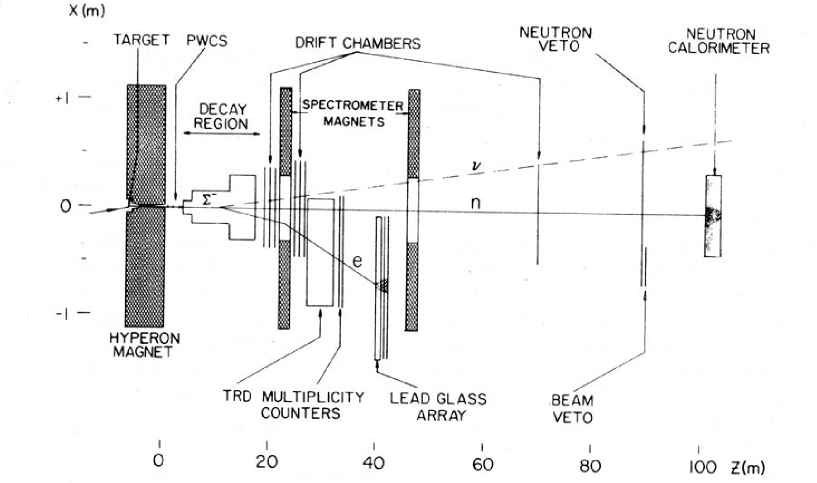
Figure 1: Plan view of the E715 apparatus, with typical particle trajectories. The incident proton-beam angle corresponds to a positive targeting angle in the horizontal plane. Note that the X and Z scales are different.

A plan view of the E715 experimental apparatus is shown in Fig. 1. The experiment E715 was performed using the Fermilab Proton Center charged-hyperon beam. Polarized hyperons were copiously produced at a nominal momentum of 250 $\mathrm{GeV}/\mathrm{c}$. Changing the direction of the incident 400 $\mathrm{GeV}/\mathrm{c}$ proton beam readily altered the hyperon polarization direction. At an average production angle of 2.5 mrad, the measured $\Sigma^{-}$ polarization was $(23.6\pm 4.3)\%$.

To distinguish the relatively rare beta-decay mode, $\Sigma^{-}\rightarrow n\,e^{-}\overline{\nu}\,\,$, from the dominant $\Sigma^{-}\rightarrow n\pi^{-}$ mode, the experiment employed double electron identification with a 12-plane transition radiation detector (TRD) and a four-layer lead-glass calorimeter array. High-pressure proportional chambers determined $\Sigma^{-}$ trajectories, and a drift-chamber magnetic spectrometer measured the momenta of charged decay products. A neutron calorimeter located far downstream provided energy and direction measurements for the decay neutrons, allowing a full reconstruction of the beta decays. A sample of 49,671 candidate beta decays contained a background of less than 2%.

The ability to reverse the $\Sigma^{-}$ polarization (by alternating positive and negative targeting angles) made possible the use of bias-canceling techniques to determine $\alpha_{e}$, $\alpha_{\nu}$, and $\alpha_{n}$ values as given in Table 4. In fact, some data were even recorded with the $\Sigma^{-}$ polarization perpendicular to the vertical hyperon magnet field, and the precession in the magnetic field used to determine the $\Sigma^{-}$ magnetic moment Zapalac with both two-body decays and beta decays.

The form factor ratios $|g_{1}/f_{1}|$ and $f_{2}/f_{1}$ were determined most sensitively from the neutron and electron spectra respectively in the $\Sigma^{-}$ rest frame yielding $|g_{1}/f_{1}-0.237g_{2}/f_{1}|=0.327\pm 0.020$ and $f_{2}/f_{1}=-0.96\pm 0.15$. A general fit that included the asymmetry parameters and made the conventional assumption $g_{2}=0$ gave the final value $g_{1}/f_{1}=-0.328\pm 0.019$. As Table 4 and the final value for $g_{1}/f_{1}$ show, this experiment unambiguously resolved the controversy concerning the sign of $g_{1}/f_{1}$ in favor of the Cabibbo model prediction.

3.3 $\Lambda\rightarrow pe^{-}\overline{\nu}_{e}$ 

(a) Brookhaven National Laboratory AGS experiment: This landmark experiment WiseLambda provided the first high statistics study of lambda beta decay. The neutral beam was derived at $4^{o}$ with respect to the primary proton beam, so that the lambdas were produced polarized. However, the polarization information was not used in the subsequent analysis. A sweeping magnet removed charged particles in the manner characteristic of hyperon beam arrangements, and a 10 radiation length lead filter removed photons leaving a neutral beam consisting mainly of lambdas, kaons and neutrons. The spectrometer consisted of two analyzing magnets and spark chambers to measure the laboratory momenta of the two charged decay particles with comparable precision. Four threshold Cerenkov counters were used for particle identification. The data sample after cuts consisted of slightly over 10,000 $\Lambda\rightarrow pe^{-}\overline{\nu}_{e}$ and 25,000 $\Lambda\rightarrow p\,\pi^{-}$events. This yielded a precision measurement of the branching ratio: BR = $\mbox{$\Lambda\rightarrow pe^{-}\overline{\nu}_{e}$}\,/\mbox{$\Lambda\rightarrow p\,\pi^{-}$}=(0.843\pm 0.017)10^{-3}$. Using the world average for the lifetime known at that time PDG78 the absolute rate for $\Lambda^{0}$ beta decay can be derived: $\Gamma(\mbox{$\Lambda\rightarrow pe^{-}\overline{\nu}_{e}$}\,)=(3.204\pm 0.068)\,10^{-3}s^{-1}$. The form factor analysis was made on the basis of the Dalitz plot that reflects the electron neutrino angular correlation. Although the lambdas were produced in principle polarized, this information was not used because the targeting angle was not reversed. This precluded making use of the bias canceling technique subsequently used to advantage by the $\Sigma^{-}\rightarrow n\,e^{-}\overline{\nu}\,\,$experiment JensenPrivate . Without polarization correlations the form factor result is a linear combination of $g_{1}$ and $g_{2}$ that the authors give as $|g_{1}/f_{1}|=0.715+0.25g_{2}/f_{1}$. In the final result, the form factor $g_{2}$ is set to zero and the final result given as $|g_{1}/f_{1}|=0.715\pm 0.026$. With these provisos, the form factor results are:

$$f_{1}=1.238\pm 0.024,\;|g_{1}|=0.885\pm 0.030,\;f_{2}=1.34\pm 0.20.$$

The values stated are extrapolated to $q^{2}=0$ and modified for radiative corrections. Although the sign of the form factors cannot be readily deduced from unpolarized data, the sign of $g_{1}$ can be safely set to be positive on the basis of earlier lower statistics experiments that measured correlations with lambda polarization Lindquist . The determination of $|g_{1}/f_{1}|$ from the Dalitz plot in the Brookhaven experiment does not depend on the value of $f_{2}$.

(b) Fermilab neutral hyperon beam: This experiment dwo is the highest statistics measurement of $\Lambda\rightarrow pe^{-}\overline{\nu}_{e}$ to date, having analyzed nearly 40,000 events. In conception this experiment has many similarities with the BNL one. A sweeping magnet removed charged particles, a characteristic feature of hyperon beams. Both a threshold Cerenkov counters and a lead-glass array were used for particle identification. The spectrometer consisted of an analyzing magnet and multiwire proportional chambers to measure the laboratory momenta of the two charged decay particles. Again, the polarization information is not used in the data analysis. There is however a noteworthy innovation in the event reconstruction. Typically, the $\Lambda^{0}$ momentum (hence the neutrino momentum) is reconstructed with a two-fold ambiguity because the $\Lambda^{0}$ direction in the laboratory is well-known, but the energy is not. Thus, in fitting for $\Lambda\rightarrow pe^{-}\overline{\nu}_{e}$ there is a two-fold ambiguity in the angle $\cos\theta^{*}_{e\nu}$ between the electron and anti-neutrino in the lambda rest frame, which diminishes its analyzing power. The authors point out that there is no ambiguity in the momentum of the proton-electron system considered as a fictitious particle, $\mathcal{Q}$. Thus the decay sequence is $\Lambda^{0}\rightarrow\mathcal{Q}+\bar{\nu}$ and $\mathcal{Q}\rightarrow p+e$. In the laboratory system, consider a plane P perpendicular to the direction of the neutral beam. By momentum conservation, the intersections of $\mathcal{Q},p,e$ with this plane are collinear, as are the intersections of $\Lambda^{0},\mathcal{Q},\bar{\nu}$. Since there is no twofold kinematic ambiguity in these lines of intersection, the distribution of the included angle is more sensitive to $|g_{1}/f_{1}|$ than the distribution in $\cos\theta^{*}_{e\nu}$. This method of analysis was used to advantage in a succeeding experiment on $\Xi^{0}\rightarrow\Sigma^{+}\,e^{-}\,\overline{\nu}_{e}\,\,$​​; we will discuss it more extensively in the section dedicated to that experiment.

The result for the form factors is: $|g_{1}/f_{1}|=0.731\pm 0.016$. While the result is given with positive sign on the basis of a slight sensitivity of induced terms to sign, we prefer to rely on experiments that include polarization correlation, where the effects are large. The caveats with respect to $g_{2}$ dependence apply, and this form factor is set to zero as in the BNL experiment. The values stated are extrapolated to $q^{2}=0$ and modified for radiative corrections. In addition, a value for the weak magnetism form-factor is given: $f_{2}/f_{1}=0.15\pm 0.30$. This is quite far from the expected value of $f_{2}/f_{1}\approx 1$. In fact, if one uses the expected value for $f_{2}$, the result changes slightly: $|g_{1}/f_{1}|=0.719\pm 0.016\pm 0.012$.

(c) CERN SPS Charged-Hyperon Beam: An experiment at the charged-hyperon beam at CERN collected over 7,000 $\Lambda\rightarrow pe^{-}\overline{\nu}_{e}$ events among a number of charged hyperon beta decay channels. Bourquin:1983I . The experiment is well-described in Gaillard:1984ny . We summarize it here for completeness. The lambdas arise from $\Xi^{-}\rightarrow\Lambda^{0}\pi^{-}$ decays, so that each $\Lambda^{0}$ is tagged. This gives the charged-hyperon beam an advantage over neutral beams where $K^{0}$ decays, and in particular $K^{0}\rightarrow\pi^{+}e^{-}\bar{\nu}$, can be a significant source of background. Electron identification relied on both lead glass and transition radiation detectors to suppress the dominant 2-body decay mode of the $\Lambda^{0}$. The form-factor analysis made use of baryon kinetic energy, electron kinetic energy, Dalitz plot and electron-neutrino correlation. Moreover, the $\Lambda^{0}$ is polarized with an asymmetry parameter of $\alpha=-0.456\pm 0.014$ PDG2002 , so that $g_{1}$ can be determined both in magnitude and sign. The result is $g_{1}/f_{1}=0.70\pm 0.03$ with $g_{2}$ taken to be 0. Otherwise, the sensitivity to $g_{2}$ is stated as $\Delta g_{1}/\Delta g_{2}=0.20$. The weak magnetism form-factor was derived from the electron spectrum to have the value $f_{2}/f_{1}=1.32\pm 0.81$ . The values stated are extrapolated to $q^{2}=0$ and modified for radiative corrections.

3.4 $\Xi^{0}\rightarrow\Sigma^{+}\,e^{-}\,\overline{\nu}_{e}\,\,$

This may appropriately be called “the last hyperon beta decay.” It is the last of observable beta decays of the octet to be measured. The experiment was long considered sufficiently problematic to be below the radar of most compilations. A notable exception was the original Cabibbo proposal cab . Paradoxically, this is in some respects the most accessible beta decay. The $\Sigma^{+}\,$is a unique signature for the beta decay mode (the analog two-body mode is forbidden by energy conservation) so that event samples are remarkably free of two-body backgrounds that typically plague experiments. Moreover, the final-state $\Sigma^{+}\,$polarization is self-analyzing because of the large asymmetry of the decay $\Sigma^{+}\rightarrow p\,\pi^{0}$  ($\alpha=-0.98$). It is thus sufficient to study angular correlations with the proton. However, attaining sufficient event rate required a new generation of hyperon experiments that combine the high-energy advantages of hyperon beams with the high phase space acceptance of neutral kaon beams. Beams with the desired properties arose in the context of recent precision studies of $CP$ violation in neutral kaon decays e'ktev ; Lai:2001ki . In place of the narrow phase-space selection of a hyperon beam magnet, the new experiments use an identifying feature of either the production or decay process. In effect, the event is “tagged.” In the case of the decay $\Xi^{0}\rightarrow\Sigma^{+}\,e^{-}\,\overline{\nu}_{e}\,\,$, only the beta decay mode has sufficient $Q$-value to produce a $\Sigma^{+}\,$​​. Identified $\Xi^{0}\rightarrow\Lambda\,\pi^{0}$ can be used as the primary source for the study of $\Lambda\,$decay.

The KTeV experiment (Fermilab E799) reported the first observation cb of the decay $\Xi^{0}\rightarrow\Sigma^{+}\,e^{-}\,\overline{\nu}_{e}\,\,$, followed by a measurement of the form factors ffcb . The KTeV neutral beam is produced by an 800 $\mathrm{GeV/c}$ proton beam hitting a 30 $\mathrm{cm}$ BeO target at an angle of 4.8 $\mathrm{mrad}$. The sweeping magnets used to remove charged particles from the neutral beam also serve to precess the polarization of the $\Xi^{0}\,$to the vertical direction. The polarity of the final sweeping magnet is regularly flipped so as to have equal numbers of $\Xi^{0}\,$polarized in opposite directions, making the ensemble average of the $\Xi^{0}\,$polarization negligible. The presence of both a CsI electromagnetic calorimeter and a system of transition radiation detectors (TRD) permitted double electron identification, a useful feature in beta decay experiments.

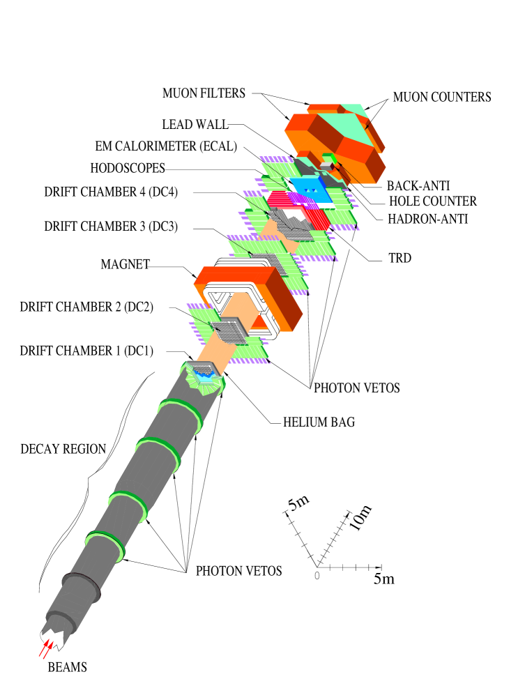
Figure 2: The KTeV Detector

Figure 3: The $\Sigma^{+}\rightarrow p\,\pi^{0}$  mass peak, after all selection criteria have been applied. The background to the left of the peak is due to $\Xi^{0}\rightarrow\Lambda\,\pi^{0}$ decays ( followed by $\Lambda\rightarrow p\,\pi^{-}$or $\Lambda\rightarrow pe^{-}\overline{\nu}_{e}$ ). Since $\Xi^{0}\rightarrow\Sigma^{+}\,e^{-}\,\overline{\nu}_{e}\,\,$is the only source of $\Sigma^{+}\,$in the beam ($\Xi^{0}\rightarrow\Sigma^{+}\,\pi^{-}\,$is kinematically forbidden), signal events are identified by having a $p$-$\pi^{0}\,$mass within 15 $\mathrm{MeV}$ of the nominal $\Sigma^{+}\,$mass.

Since the neutrino is unobserved, one cannot unambiguously reconstruct the directions in the center of mass. Instead one can obtain unambiguous angular variables transverse to the direction of the $\Xi^{0}\,$momentum. Following Dworkin dwo , we consider the decay sequence

$$\mbox{$\Xi^{0}\,$}\rightarrow Q+\overline{\nu_{e}},\,\,\,Q\rightarrow\mbox{$\Sigma^{+}\,$}+e^{-}$$ (33)

where we have introduced the fictitious particle $Q$. We then construct angular variables out of these transverse quantities. Denoting quantities in the $Q$ rest frame with an asterisk, we have the transverse momenta of the electron, proton, and neutrino in the $Q$ frame: ${\vec{p}}_{e\perp}^{*}$, ${\vec{p}}_{p\perp}^{*}$ and ${\vec{p}}_{\nu\perp}$. The magnitudes of the momenta in the $Q$ frame are calculated to obtain the unambiguous kinematic quantities

$$\mbox{$x_{e\nu\perp}$}=\frac{{\vec{p}}_{e\perp}^{*}\cdot{\vec{p}}_{\nu\perp}}{{E_{e}}^{*}{E_{\nu}}^{*}}$$ (34)

and

$$\mbox{$x_{p\nu\perp}$}=\frac{{\vec{p}}_{p\perp}^{*}\cdot{\vec{p}}_{\nu\perp}}{\mid{\vec{p}}_{p}^{*}\mid{E_{\nu}}^{*}}$$ (35)

which correspond to the polarization of the $\Sigma^{+}\,$along the neutrino direction, and the electron-neutrino correlations respectively. The kinematic quantity corresponding to the proton-electron correlation is $x_{pe}$, the cosine of the angle between the proton and the electron in the $\Sigma^{+}\,$frame. The one dimensional distributions for $x_{pe}$, $x_{e\nu\perp}$ and $x_{p\nu\perp}$ are shown in Fig. 4.

Figure 4: The three variables used to fit $g_{1}/f_{1}\,$and $g_{2}/f_{1}\,$, and the energy spectrum of the electron in the $\Sigma^{+}\,$frame (used to determine $f_{2}/f_{1}\,$). The points are data and the histogram is a Monte Carlo simulation with $g_{1}/f_{1}\,$$=1.27$ and $\mbox{$g_{2}/f_{1}\,$}=0.$

To determine $g_{1}/f_{1}\,$​, a maximum likelihood fit for $g_{1}/f_{1}\,$using $x_{pe}$, $x_{p\nu\perp}$  and $x_{e\nu\perp}$  is performed. After correcting for background, the final value for $g_{1}/f_{1}\,$is $1.32\pm^{0.21}_{0.17}(\mathrm{stat})$(Fig. 5). As a check of the Monte Carlo simulation, the two body asymmetry product $\alpha_{\Xi}\alpha_{\Lambda}$is determined with a sample of $70,000$ $\Xi^{0}\rightarrow\Lambda\,\pi^{0}$ events. The measured $\alpha_{\Xi}\alpha_{\Lambda}$$=-0.286\pm 0.008(\mathrm{stat})\pm 0.015(\mathrm{syst})$ is consistent with the Particle Data Group value of $-0.264\pm 0.013$ PDG2002 .

Figure 5: Confidence interval plot for $f_{1}$ and $g_{1}$. The inverted triangle is exact SU(3) symmetry; the star indicates the KTeV value. Solid circles and squares are SU(3) breaking fits from rat and Flores-Mendieta:1998ii respectively.

Relaxing the requirement that $g_{2}=0$, and fitting the distributions to $g_{1}/f_{1}\,$and $g_{2}/f_{1}\,$  simultaneously, one finds no evidence for a non-zero second class current term (Fig. 6), measuring $\mbox{$g_{1}/f_{1}\,$}=1.17\pm{0.28}(stat)\pm 0.05(syst)$ and $\mbox{$g_{2}/f_{1}\,$}=-1.7\pm^{2.1}_{2.0}(stat)\pm 0.5(syst)$.

Figure 6: Maximum likelihood fit to $g_{2}/f_{1}\,$and $g_{1}/f_{1}\,$.

Using the measured $g_{1}/f_{1}\,$​, and assuming $\mbox{$g_{2}/f_{1}\,$}=0$, one then determines the value for $f_{2}/f_{1}\,$using the electron energy spectrum in the $\Sigma^{+}\,$frame ( Fig. 4). (The electron spectrum is the only kinematic quantity that depends on $f_{2}/f_{1}\,$to lowest order in $(M_{\Xi^{0}}-M_{\Sigma^{+}})/M_{\Xi^{0}}$.) A maximum likelihood fit yelds the value $f_{2}/f_{1}\,$= $2.0\pm 1.2(\mathrm{stat})\pm 0.5(\mathrm{syst})$.

To summarize, the KTeV experiment made the first measurement of $g_{1}/f_{1}\,$for the decay $\Xi^{0}\rightarrow\Sigma^{+}\,e^{-}\,\overline{\nu}_{e}\,\,$​​, and found that $\mbox{$g_{1}/f_{1}\,$}=\mbox{$1.32\pm^{0.21}_{0.17}(\mathrm{stat})\pm 0.05(syst)$}$ assuming that no second class current is present and that the weak magnetism term has the exact $SU(3)\,$value. By using the electron–neutrino correlation and the final state polarization of the $\Sigma^{+}\,$observed via its two body decay $\Sigma^{+}\rightarrow p\,\pi^{0}$, one was able to determine both the sign and magnitude of $g_{1}/f_{1}\,$​. The answer is consistent with the exact $SU(3)\,$prediction, and $SU(3)\,$breaking schemes in which only $g_{1}$ is allowed to be modified from its exact $SU(3)\,$value. Predictions that allow for the renormalization of $f_{1}$ are disfavored. Furthermore, removing the constraint that $g_{2}=0$, and simultaneously fitting for $g_{1}/f_{1}\,$and $g_{2}/f_{1}\,$​​, reveals no evidence for a second-class current term. The analysis of the energy spectrum of the electron in the $\Sigma^{+}\,$frame gives a value for $f_{2}/f_{1}\,$that is consistent with the $SU(3)\,$prediction.

Outlook and future prospects: (a) $\Xi^{0}\rightarrow\Sigma^{+}\,e^{-}\,\overline{\nu}_{e}\,\,$: The KTeV experiment collected a factor of four more data in 1999. While analysis is still in progress, one can already get a sense of the data quality from the $\Sigma^{+}\,$mass plot shown in Fig. 7.

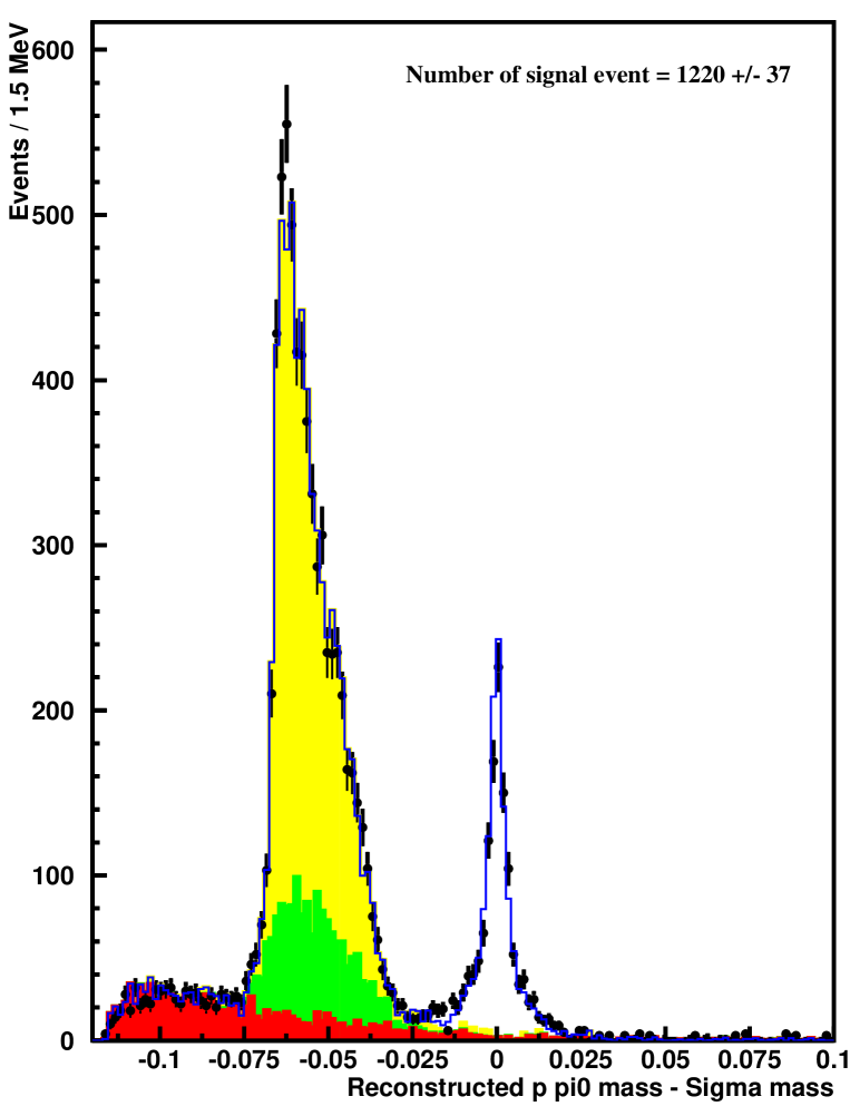
Figure 7: The $\Sigma^{+}\rightarrow p\,\pi^{0}$  mass peak after all selection criteria have been applied. The background to the left of the peak is due to $\Xi^{0}\rightarrow\Lambda\,\pi^{0}$ decays ( followed by $\Lambda\rightarrow p\,\pi^{-}$or $\Lambda\rightarrow pe^{-}\overline{\nu}_{e}$ ). Since $\Xi^{0}\rightarrow\Sigma^{+}\,e^{-}\,\overline{\nu}_{e}\,\,$is the only source of $\Sigma^{+}\,$in the beam ($\Xi^{0}\rightarrow\Sigma^{+}\,\pi^{-}\,$is kinematically forbidden), signal events are identified by having a $p$-$\pi^{0}\,$mass within 15 $\mathrm{MeV}$ of the nominal $\Sigma^{+}\,$mass.

Similarly, one gets an appreciation of the improved sensitivity from a mass plot of anti $\Sigma^{+}\,$shown in Fig. 8. This is a first observation of anti $\Xi^{0}\,$beta decay.

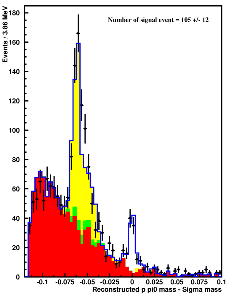
Figure 8: $\bar{\Sigma}^{+}$ mass plot from $\bar{\Xi}^{0}$ beta decay after all selection criteria have been applied. The background to the left of the peak appears larger as a result of the smaller cross section for anti $\Xi^{0}\,$production.

The CERN NA 48 experiment reported a sample of 60 $\Xi^{0}\,$beta decay candidates at the 2000 High Energy Physics Conference in Osaka. Based on this, a succeeding data run with somewhat improved instrumentation and trigger is planned for 2002-2004 with the expectation of collecting some 25,000 beta decay events. This will represent a significant advance in the precision study of hyperon beta decay.

(b) $\Lambda\rightarrow pe^{-}\overline{\nu}_{e}$ : An important advantage of working with intense neutral beams is the possibility of using “tagged” $\Lambda$’s from $\Xi^{0}\rightarrow\Lambda\,\pi^{0}$ decays to study $\Lambda^{0}$ beta decay, with the double advantage of mitigating the presence of a $Ke_{3}$ background and of $\Lambda$’s which are 40% polarized. The KTeV data from 1999 are expected to have some 5,000 $\Lambda\rightarrow pe^{-}\overline{\nu}_{e}$ from this source. In addition the forthcoming NA48 run at CERN in 2002-2004 can increase this sample by an order of magnitude. Thus a new level of precision in the $\Lambda\rightarrow pe^{-}\overline{\nu}_{e}$ parameters appears to be within reach.

3.5 Neutron decay

Measurements of neutron beta decay date back to the classic experiments of Robson with unpolarized neutrons Robson and of Burgy, Krohn, Novey, Ringo, and Telegdi with polarized neutrons Burgy . Modern experiments have measured the neutron lifetime and decay distribution parameters PDG2002 with levels of precision much greater than those achieved in hyperon decay experiments. First-order recoil effects (arising from terms containing $f_{2}$ and $g_{2}$) may even be detectable Gardner in the near future. At present, six precise measurements of the neutron lifetime give consistent results yielding an average of $(885.7\pm 0.8)$s PDG2002 ; Pendelbury . Clearly the opportunity to study trapped neutrons has greatly advanced the ability to perform these measurements.

Five contemporary experiments with polarized neutrons yield an average of $\alpha_{e}=-0.1162\pm 0.0013$ and a form factor ratio $(g_{1}/f_{1})_{n}=1.2670\pm 0.0030$ PDG2002 . These five measurements are not statistically consistent ($\chi^{2}/d.f.=10.5/4$) leading to an error scale factor of S = 1.6. The inconsistency arises from the conflict between the published PERKEO II result $(g_{1}/f_{1})_{n}=1.274\pm 0.003$ Abele and the other four results Liaud (average of $(g_{1}/f_{1})_{n}=1.2637\pm 0.0021$). A new PERKEO II measurement AbeleII exactly confirms their earlier result and yields $(g_{1}/f_{1})_{n}=1.2739\pm 0.0019$. The new experiment has the particular merit that the total correction to the raw data is only 2%, some 10 times smaller than in earlier experiments. This new result reinforces the inconsistency. Combining it with the other five results, we obtain an average of $(g_{1}/f_{1})_{n}=1.2680\pm 0.0026$ with $\chi^{2}/d.f.=12.4/5$ and S = 1.6. When comparing hyperon beta decay results to the Cabibbo model, the value of $(g_{1}/f_{1})_{n}$ provides us with a powerful constraint : $F+D=(g_{1}/f_{1})_{n}=1.2670\pm 0.0030$. For consistency, we choose to use the 2002 Particle Data Group average. In this context the difference between the PERKEO II results and those of earlier experiments is of little consequence. On the other hand, this difference is relatively important when determining $V_{ud}$ from the neutron lifetime and $(g_{1}/f_{1})_{n}$ AbeleII ; Towner .

4 Cabibbo-Model Fits

The Ademollo-Gatto Theorem suggests an analytic approach to the available data that first examines the vector form factor $f_{1}$ because it is not subject to first-order $SU(3)$  symmetry breaking effects. An elegant way to do this is to use the measured value of $g_{1}/f_{1}$ along with the predicted values of $f_{1}$ and $f_{2}$ (see Table 1) to extract a $V_{us}$ value from the decay rate for each decay. Consistency of the $V_{us}$ values obtained from different decays then indicates the success of the Cabibbo model.

Four hyperon beta decays have sufficient data to perform this analysis: $\Lambda\rightarrow p\,e^{-}\bar{\nu},\;\Sigma^{-}\rightarrow n\,e^{-}\bar{\nu},\;\Xi^{-}\rightarrow\Lambda\,e^{-}\bar{\nu},\;\Xi^{0}\rightarrow\Sigma^{+}\,e^{-}\bar{\nu}$. Table 5 shows the results for them. In this analysis, both model-independent and model-dependent radiative corrections GarciaBook are applied and q² variation of f₁ and g₁ is included. Also $SU(3)$  values g₂ = 0 and f₂ as given in Table 1 are used along with the numerical rate expressions tabulated in Ref. GarciaBook . The four values are clearly consistent ($\chi^{2}=2.26/3$d.f.) with the combined value of $V_{us}$ = 0.2250 $\pm$ 0.0027. This value is nearly as precise as that obtained from kaon decay ($V_{us}$ = 0.2196 $\pm$ 0.0023) and, as suggested by previous analyses Gaillard:1984ny ; highvus ; Flores-Mendieta:1998ii , is somewhat larger. In combination with $V_{ud}$ = 0.9740 $\pm$ 0.0005 obtained from superallowed pure Fermi nuclear decays Towner , the larger $V_{us}$ value from hyperon decays beautifully satisfies the unitarity constraint |$V_{ud}$|² + |$V_{us}$|² + |$V_{ub}$|² = 1. As discussed extensively by Towner and Hardy Towner , the unitarity constraint falls short by 2.2 standard deviations with the smaller kaon decay value.

Table 5: Results from $V_{us}$ analysis using measured $g_{1}/f_{1}$ values

Decay	Rate	$g_{1}/f_{1}$	$V_{us}$
Process	($\mu sec^{-1}$)
$\Lambda\rightarrow pe^{-}\overline{\nu}$	$3.161(58)$	$0.718(15)$	0.2224 $\pm$ 0.0034
$\Sigma^{-}\rightarrow ne^{-}\overline{\nu}$	$6.88(24)$	$-0.340(17)$	0.2282 $\pm$ 0.0049
$\Xi^{-}\rightarrow\Lambda e^{-}\overline{\nu}$	$3.44(19)$	$0.25(5)$	0.2367 $\pm$ 0.0099
$\Xi^{0}\rightarrow\Sigma^{+}e^{-}\overline{\nu}$	$0.876(71)$	$1.32(+.22/-.18)$	0.209 $\pm$ 0.027
Combined	—	—	0.2250 $\pm$ 0.0027

First order $SU(3)$  symmetry breaking effects are expected to manifest themselves in g₁/f₁. The newly measured decay $\Xi^{0}\rightarrow\Sigma^{+}\,e^{-}\bar{\nu}$ provides a direct test because it is predicted to have the same form factor ratio as the well-measured neutron beta decay: $n\rightarrow p\,e^{-}\bar{\nu}$. As shown in Table 3, the results are consistent with this prediction, but the errors are currently rather large. For the other decays, it is necessary to fit for the reduced axial-vector form factors $F$ and $D$. Since $g_{1}/f_{1}=F+D$ for neutron beta decay, this combination is very well determined. It is therefore better to fit for the linear combinations $F+D$ and $F-D$ which will then have essentially uncorrelated errors. This fit yields $F+D=1.2670\,\pm 0.0030$ and $F-D=-0.341\pm 0.016$ with $\chi^{2}=2.96/3$ d.f. As might be expected, the result for F - D is dominated by the reasonably precise $g_{1}/f_{1}$ value for $\Sigma^{-}\rightarrow n\,e^{-}\bar{\nu}$. Surprisingly, even with today’s improved measurements, no clear evidence of $SU(3)$  symmetry breaking effects emerges. They appear to be much smaller than expected.

The value for $V_{us}$ determined from hyperon beta decays, without applying any $SU(3)$  breaking corrections to $f_{1}$, but including radiative corrections, is:

$$V_{us}=0.2250\,(27)\quad\text{hyperon beta decay}$$ (36)

The expected negative correction to $f_{1}$ would drive this higher, to

$$V_{us} =0.2279\,(27)\quad\text{Ref. \cite[cite]{\@@bibref{Authors Phrase1YearPhrase2}{Donoghue:th}{\@@citephrase{(}}{\@@citephrase{)}}}}$$ (37)

$$V_{us} =0.2307\,(27)\quad\text{Ref. \cite[cite]{\@@bibref{Authors Phrase1YearPhrase2}{Schlumpf:1994fb}{\@@citephrase{(}}{\@@citephrase{)}}}}$$

The accepted value from $K_{l3}$ decays, including corrections from chiral perturbation theory, Leutwyler , is considerably lower,

$$V_{us}=0.2196\,(23)\quad K_{l3}\text{ decay}$$ (38)

We have a puzzle: why are the two values different? If we assume that the $f_{1}$ correction in hyperon beta decays must be negative, Eq. (36) must be considered a lower limit for $V_{us}$. We are thus driven to the conclusion that the value from $K_{l3}$ is an underestimate. Is this possible? Perhaps yes: a quark-model computation Jaus of the $F_{+}(0)$ correction in $K_{l3}$ finds $F_{+}(0)=0.965$. While at first sight this is compatible with the chiral perturbation theory Leutwyler result, $F_{+}(0)=0.961$, it is not evident that the two computations reflect the same corrections. It could well be that the two corrections should, at least in part, be combined. In other words it is possible that chiral perturbation theory neglects some short-distance contribution which is well described by the quark model, and this would explain the discrepancy between the two results.

While it is clear that more theoretical work is needed to fully clarify the situation, we are at this point convinced that there is no reason to prefer the $K_{l3}$ result over the one derived from hyperon beta decays. Indeed there is now also a preliminary experimental indication Sher that the $K_{e3}$ decay rate may be higher than the value used to obtain Eq. (38).

5 Conclusions and Open Questions

The determination of the elements of the CKM matrix is one of the main ingredients for evaluating the solidity of the standard model of elementary particles. This is a vast subject which has seen important progress with the determination of $\epsilon^{\prime}/\epsilon$ and the observation of $CP$ violation in B decays.

While a lot of attention has recently been justly devoted to the higher mass sector of the CKM matrix, it is the low mass sector, in particular $V_{ud}$ and $V_{us}$ where the highest precision can be attained, and which can provide the most sensitive test of the unitarity of the CKM matrix through the relation $|V_{ud}|^{2}+|V_{us}|^{2}+|V_{ub}|^{2}=1$. Given the fact that the $|V_{ub}|^{2}$ contribution is totally negligible, the unitarity test reduces to the consistency of $\cos\theta_{C}$ determined from nuclear beta decay and of $\sin\theta_{C}$ determined from strangeness changing semileptonic decays.

In the present review we have reconsidered the contribution that the hyperon beta decays can give to the determination of $\sin\theta_{C}$. The conventional analysis of hyperon beta decay in terms of the $F,D$ and $\sin\theta_{C}$ parameters is marred by the expectation of first order $SU(3)$ breaking effects in the axial-vector contribution. The situation is only made worse if one introduces adjustable $SU(3)$ breaking parameters as this increases the number of degrees of freedom and degrades the precision. If on the contrary, as we did here, one focuses the analysis on the vector form factors, treating the rates and $g_{1}/f_{1}$ as the basic experimental data, one has direct access to the $f_{1}$ form factor for each decay, and this in turn allows for a redundant determination of $\sin\theta_{C}$. The consistency of the values of $\sin\theta_{C}$ determined from the different decays is a first confirmation of the overall consistency of the model.

The value of $\sin\theta_{C}$ obtained from hyperon decays is of comparable precision with that obtained from $K_{l3}$ decays, and is in better agreement with the value of $\theta_{C}$ obtained from nuclear beta decay. While a discrepancy between $V_{us}$ and $V_{ud}$ could be seen as a portent of exciting new physics, a discrepancy between the two different determinations of $V_{us}$ can only be taken as an indication that more work remains to be done both on the theoretical and the experimental side.

On the theoretical side, renewed efforts are needed for the determination of $SU(3)$  ​​-breaking effects in hyperon beta decays as well as in $K_{l3}$ decays. While it is quite possible to improve the present situation on the quark-model front, the best hopes lie in lattice QCD simulations, perhaps combined with chiral perturbation theory for the evaluation of large-distance multiquark contributions.

We have given some indication that the trouble could arise from the $K_{l3}$ determination of $\sin\theta_{C}$, and we would like to encourage further experimental work in this field. We are however convinced of the importance of renewed experimental work on hyperon decays, of the kind now in progress at the CERN SPS. The interest of this work goes beyond the determination of $\sin\theta_{C}$, as it involves the intricate and elegant relationships that the model predicts.

6 Acknowledgements

With permission from the Annual Review of Nuclear and Particle Science. Final version of this material is scheduled to appear in the Annual Review of Nuclear and Particle Science Vol. 53, to be published in December 2003 by Annual Reviews, http//AnnualReviews.org. The idea for undertaking this review arose during Hyperon 99 at Fermilab. We are grateful to D. A. Jensen and E. Monnier for organizing this stimulating conference. The continuing intellectual stimulation provided by colleagues in the Fermilab KTeV Collaboration, particularly members of the hyperon working group, is gratefully acknowledged. We thank J. L. Rosner for a thorough and thoughtful reading of our manuscript. This work was supported in part by the U.S. Department of Energy under grant DE-FG02-90ER40560 (Task B).

Appendix A Appendix

We present the analytic expressions for the integrated final state polarization to order $\delta^{2}$ in the final state rest frame, assuming real form factors.

$$R = R_{0}[(1-\frac{3}{2}\delta)\mbox{$f_{1}^{2}$}+(3-\frac{9}{2}\delta)\mbox{$g_{1}^{2}$}-(4\delta)\mbox{$g_{1}g_{2}$}]+R(\delta^{2}),$$

$$R\mathsf{S}_{e} = R_{0}[(2-\frac{10}{3}\delta)\mbox{$g_{1}^{2}$}+(2-\frac{7}{3}\delta)\mbox{$f_{1}g_{1}$}-(\frac{1}{3}\delta)\mbox{$f_{1}^{2}$}$$

$$-(\frac{2}{3}\delta)\mbox{$f_{1}f_{2}$}+(\frac{2}{3}\delta)\mbox{$f_{2}g_{1}$}-(\frac{2}{3}\delta)\mbox{$f_{1}g_{2}$}-(\frac{10}{3}\delta)\mbox{$g_{1}g_{2}$}]+R\mathsf{S}_{e}(\delta^{2}),$$

$$R\mathsf{S}_{\nu} = R_{0}[(-2+\frac{10}{3}\delta)\mbox{$g_{1}^{2}$}+(2-\frac{7}{3}\delta)\mbox{$f_{1}g_{1}$}+(\frac{1}{3}\delta)\mbox{$f_{1}^{2}$}$$

$$+(\frac{2}{3}\delta)\mbox{$f_{1}f_{2}$}+(\frac{2}{3}\delta)\mbox{$f_{2}g_{1}$}-(\frac{2}{3}\delta)\mbox{$f_{1}g_{2}$}+(\frac{10}{3}\delta)\mbox{$g_{1}g_{2}$}]+R\mathsf{S}_{\nu}(\delta^{2}),$$

$$R\mathsf{S}_{\alpha} = R_{0}[(\frac{8}{3}-\frac{52}{15}\delta)\mbox{$f_{1}g_{1}$}+(\frac{16}{15}\delta)\mbox{$f_{2}g_{1}$}-(\frac{16}{15}\delta)\mbox{$f_{1}g_{2}$}]+R\mathsf{S}_{\alpha}(\delta^{2}),$$

$$R\mathsf{S}_{\beta} = R_{0}[(\frac{8}{3}-4\delta)\mbox{$g_{1}^{2}$}-(\frac{8}{15}\delta)\mbox{$f_{1}^{2}$}-(\frac{16}{15}\delta)\mbox{$f_{1}f_{2}$}$$ (39)

$$-(\frac{64}{15}\delta)\mbox{$g_{1}g_{2}$}]+R\mathsf{S}_{\beta}(\delta^{2}),$$

where

$$R_{0}=\frac{G_{S}^{2}(\delta M_{B})^{5}}{60\pi^{3}}.$$

$$R(\delta^{2}) = R_{0}\delta^{2}(\frac{6}{7}\mbox{$f_{1}^{2}$}+\frac{12}{7}\mbox{$g_{1}^{2}$}+6\mbox{$g_{1}g_{2}$}$$

$$+\frac{6}{7}\mbox{$f_{1}f_{2}$}+\frac{4}{7}\mbox{$f_{2}^{2}$}+\frac{12}{7}\mbox{$g_{2}^{2}$}),$$

$$R\mathsf{S}_{e}(\delta^{2}) = R_{0}\delta^{2}(\frac{55}{42}\mbox{$g_{1}^{2}$}+\frac{17}{21}\mbox{$f_{1}g_{1}$}+\frac{19}{42}\mbox{$f_{1}^{2}$}+\frac{4}{3}\mbox{$f_{1}f_{2}$}-\frac{10}{21}\mbox{$f_{2}g_{1}$}$$

$$+\frac{10}{21}\mbox{$f_{1}g_{2}$}+\frac{116}{21}\mbox{$g_{1}g_{2}$}+\frac{4}{21}\mbox{$f_{2}^{2}$}+\frac{4}{3}\mbox{$g_{2}^{2}$}-\frac{16}{21}\mbox{$f_{2}g_{2}$}),$$

$$R\mathsf{S}_{\nu}(\delta^{2}) = R_{0}\delta^{2}(-\frac{55}{42}\mbox{$g_{1}^{2}$}+\frac{17}{21}\mbox{$f_{1}g_{1}$}-\frac{19}{42}\mbox{$f_{1}^{2}$}-\frac{4}{3}\mbox{$f_{1}f_{2}$}-\frac{10}{21}\mbox{$f_{2}g_{1}$}$$

$$+\frac{10}{21}\mbox{$f_{1}g_{2}$}-\frac{116}{21}\mbox{$g_{1}g_{2}$}-\frac{4}{21}\mbox{$f_{2}^{2}$}-\frac{4}{3}\mbox{$g_{2}^{2}$}-\frac{16}{21}\mbox{$f_{2}g_{2}$}),$$

$$R\mathsf{S}_{\alpha}(\delta^{2}) = R_{0}\delta^{2}(\frac{316}{245}\mbox{$f_{1}g_{1}$}-\frac{752}{735}\mbox{$f_{2}g_{1}$}+\frac{752}{735}\mbox{$f_{1}g_{2}$}-\frac{128}{105}\mbox{$f_{2}g_{2}$}),$$

$$R\mathsf{S}_{\beta}(\delta^{2}) = R_{0}\delta^{2}(\frac{422}{735}\mbox{$f_{1}^{2}$}+\frac{88}{49}\mbox{$f_{1}f_{2}$}+\frac{8}{35}\mbox{$f_{2}^{2}$}$$ (40)

$$+\frac{362}{245}\mbox{$g_{1}^{2}$}+\frac{1576}{245}\mbox{$g_{1}g_{2}$}+\frac{8}{5}\mbox{$g_{2}^{2}$})$$

References

- (1) Cabibbo N. Phys. Rev. Lett. 10:531 (1963)
- (2) Kobayashi M, Maskawa T. Prog. Theor. Phys. 49:652 (1973)
- (3) Affolder A, et al (KTeV Collaboration). Phys. Rev. Lett. 82:3751 (1999)
- (4) Alavi-Harati A, et al (KTeV Collaboration). Phys. Rev. Lett. 87:132001 (2001)
- (5) Okun L. In Proc. 1958 Int. Conf. on High Energy Physics at CERN, June 30–July 5, 1958, ed. B. Ferretti, p. 223. Geneva: CERN (1958)
- (6) Sakata S. Prog. Theor. Phys. 16:686 (1956); see also, Maki Z, Nakagawa M, Sakata S. Prog. Theor. Phys. 28:870 (1962)
- (7) Berman SM. Radiative Corrections to Muon and Neutron Decay. PhD Thesis. California Institute of Technology, Pasadena, California, (1959); Berman SM. Phys. Rev. 112:267 (1958); Kinoshita T, Sirlin A. Phys. Rev. 113:1652 (1959)
- (8) Gell-Mann M, Lévy M. Nuovo Cimento 16:705 (1960)
- (9) Barbaro-Galtieri A, et al. Phys. Rev. Lett. 9:26 (1962)
- (10) Cronin J. In Proc. 14th Int. Conf. on High Energy Physics, Vienna, Aug. 28–Sept. 5, 1968, ed. Prentki J, Steinberger J, p. 281. Geneva: CERN (1968)
- (11) Hagiwara K, et al (Particle Data Group). Phys. Rev. D66:010001 (2002)
- (12) Gell-Mann M. Phys. Rev. 125:1067 (1962)
- (13) Weisberger WI. Phys. Rev. Lett. 14:1047 (1965); Adler SL. Phys. Rev. Lett. 14:1051 (1965)
- (14) Sheldon Glashow in a private communication with N Cabibbo
- (15) Alavi-Harati A, et al (KTeV Collaboration). Phys. Rev. D66:11????? (2002) [arXiv:hep-ex/0208007] ???help???
- (16) Lai A, et al (NA48 Collaboration). Eur. Phys. J. C22:231 (2001) [arXiv:hep-ex/0110019]
- (17) Aubert B, et al (BaBar Collaboration). Contributed to 31st Int. Conf. on High Energy Physics (ICHEP 2002), Amsterdam, The Netherlands, July 24–31, 2002 [arXiv:hep-ex/0207070]
- (18) Abe K, et al (Belle Collaboration). Contributed to 31st Int. Conf. High Energy Physics (ICHEP 2002), Amsterdam, The Netherlands, July 24–31, 2002 [arXiv:hep-ex/0207098]
- (19) Nir Y. Plenary talk 31st Int. Conf. High Energy Physics (ICHEP 2002), Amsterdam, The Netherlands, July 24–31, 2002 [arXiv:hep-ph/0208080]
- (20) Gaillard JM, Sauvage G. Annu. Rev. Nucl. Part. Sci. 34:351 (1984)
- (21) Bright S, Winston R, Swallow EC, Alavi-Harati A. Phys. Rev. D60:117505 (1999); see also Watson JM and Winston R. Phys. Rev. 181:1907 (1969)
- (22) Garcia A, Kielanowski R. The Beta Decay of Hyperons, Lecture Notes in Physics 222. Berlin: Springer-Verlag (1985)
- (23) Bjorken JD, Drell SD. Relativistic Quantum Mechanics. New York: McGraw-Hill (1964)
- (24) Weinberg S. Phys. Rev. 112:1375 (1958)
- (25) Primakoff H. Rev. Mod. Phys. 31:802 (1959)
- (26) Fujii A, Primakoff H. Nuovo Cimento 12:327 (1959)
- (27) Weinberg S. Phys. Rev. 115:481 (1959)
- (28) Sirlin A. Phys. Rev. 164:1767 (1967); Phys. Rev. Lett. 32:966 (1974)
- (29) Most recently, Martinez A, Torres JJ, Flores-Mendieta R, Garcia A. Phys. Rev. D63:014025 (2001) and references therein
- (30) Sirlin A. Nucl. Phys. B161:301 (1979)
- (31) Ademollo M, Gatto R. Phys. Rev. Lett. 13:264 (1964)
- (32) Fubini S, Furlan G. Physics 1:229 (1965)
- (33) Sakurai J. J. Currents and Mesons, Chicago Lectures in Physics. Chicago:University of Chicago Press (1969)
- (34) Donoghue JF, Holstein BR, Klimt SW. Phys. Rev. D35:934 (1987)
- (35) Schlumpf F. Phys. Rev. D51:2262 (1995) [arXiv:hep-ph/9409272]
- (36) Krause A. Helv. Phys. Acta 63:3 (1990)
- (37) Anderson J, Luty MA. Phys. Rev. D47:4975 (1993) [arXiv:hep-ph/9301219]
- (38) Sexton J, Weingarten D. Phys. Rev. D55:4025 (1997)
- (39) Flores-Mendieta R, Jenkins E, Manohar AV. Phys. Rev. D58:094028 (1998) [arXiv:hep-ph/9805416]
- (40) Quinn HR, Bjorken JD. Phys. Rev. 171:1660 (1968)
- (41) Holstein BR. In Hyperon 99, Proc. Hyperon Phys. Symp., Fermilab, Sept. 27-29 1999, ed. DA Jensen, E Monnier, p 4. Fermilab report FERMILAB-Conf-00/059-E (2000)
- (42) Hsueh SY, et al. Phys. Rev. D38:2056 (1988)
- (43) Oehme R, Winston R, Garcia A. Phys. Rev. D3:1618 (1971)
- (44) Cabibbo N, Chilton F. Phys. Rev. B137:1628 (1965)
- (45) Bourquin M, et al. Z. Phys. C21:17 (1983); see also Tanenbaum W, et al. Phys. Rev. D12:1871 (1975)
- (46) Keller P, et al. Phys. Rev. Lett. 48:971 (1982) and references therein; see also Garcia A, Swallow EC. Phys. Rev. Lett. 35:467 (1975)
- (47) Discussed at length in GarciaBook ; see, for example, Bohm A, Magnollay P, Garcia A, Kielanowski P. Phys. Rev. D27:180 (1983); Bohm A, Kmiecik M. Phys. Rev. D31:3005 (1985)
- (48) First observed for neutral hyperons: Bunce G, et al. Phys. Rev. Lett. 36:1113 (1976)
- (49) Lach J, Pondrom LG. Annu. Rev. Nucl. Part. Sci. 29:203 (1979)
- (50) Zapalac G, et al. Phys. Rev. Lett. 57:1526 (1986)
- (51) Wise J, et al. Phys. Lett. B91:165 (1980); Wise J, et al. Phys. Lett. B98:123 (1981)
- (52) Bricman C, et al (Particle Data Group). Phys. Lett. B75:1 (1978)
- (53) Jensen DA. private communication
- (54) See, for example, Lindquist J, et al. Phys. Rev. D16:2104 (1977)
- (55) Bourquin M, et al. Z. Phys. C21:1 (1983)
- (56) Alavi-Harati A, et al (KTeV Collaboration). Phys. Rev. Lett. 83:22 (1999)
- (57) Alavi-Harati A, et al (KTeV Collaboration). In DPF99: Proc. 1999 APS/DPF Meeting, Los Angeles, Jan. 5–9, 1999, ed. K Arisaka, Z Bern, http://www.dpf99.library.ucla.edu/session4/alavi0408.pdf
- (58) The feasibility was first studied by N. Solomey working with University of Chicago undergraduate A. Affolder
- (59) Dworkin J, et al. Phys. Rev. D41:780 (1990)
- (60) Robson J. Can. J. Phys. 36:1450 (1958)
- (61) Burgy M, Krohn V, Novey T, Ringo G, Telegdi V. Phys. Rev. 120:1827 (1960)
- (62) Gardner S, Zhang C. Phys. Rev. Lett. 86:5666 (2001)
- (63) For reviews and commentary see Pendelbury JM. Annu. Rev. Nucl. Part. Sci. 43:687 (1993); Schreckenbach J, et al. J. Phys. G18:1 (1992); Freedman SJ. Comm. Nucl. Part. Phys. 19:209 (1990)
- (64) Abele H, et al. Phys. Lett. B407:212 (1997)
- (65) Mostovoi YuA, et al. Phys. Atom. Nucl. 64:1955 (2001) [tr. YAF 64:2040 (2001)], Liaud P, et al. Nucl. Phys. A612:53 (1997); Yerozolimsky B, et al. Phys. Lett. B412:240 (1997); Bopp P, et al. Phys. Rev. Lett. 56:919 (1986)
- (66) Abele H, et al. Phys. Rev. Lett. 88:211801 (2002)
- (67) Towner IS, Hardy JC. In Proc. Vth Int. WEIN Symp.: Phys. Beyond the Standard Model, Santa Fe, NM, 1998, ed. P Herczeg, C Hoffman, HV Klapdor-Kleingrothaus, p. 338. Singapore: World Scientific (1999) [arXiv:nucl-th/9809087]
- (68) Ratcliffe PG. Phys. Rev. D59:014038 (1999)
- (69) Flores-Mendieta R, Garcia A, S’anchez-Col’on G. Phys. Rev. D54:6855 (1996); Dai J, Dashen R, Jenkins E, Manohar AV. Phys. Rev. D53:273 (1996)
- (70) Leutwyler H, Roos M. Z. Phys. C25:91 (1984)
- (71) Sher A, et al (E865 Collaboration). Contributed to DPF2002: 2002 APS/DPF Meeting, Williamsburg, Virginia, May 24–28, 2002, http://dpf2002.velopers.net/talks_pdf/332talk.pdf
- (72) Jaus W. Phys. Rev. D44:2851 (1991)