Solar Neutrino Oscillation Phenomenology

Abstract

This article summarises the status of the solar neutrino oscillation phenomenology at the end of 2002 in the light of the SNO and KamLAND results. We first present the allowed areas obtained from global solar analysis and demonstrate the preference of the solar data towards the Large-Mixing-Angle (LMA) MSW solution. A clear confirmation in favor of the LMA solution comes from the KamLAND reactor neutrino data. The KamLAND spectral data in conjunction with the global solar data further narrows down the allowed LMA region and splits it into two allowed zones – a low $\Delta m^{2}$ region (low-LMA) and high $\Delta m^{2}$ region (high-LMA). We demonstrate through a projected analysis that with an exposure of 3 kton-year (kTy) KamLAND can remove this ambiguity.

1. The Neutrinos from the sun

Solar neutrinos are produced via the reaction

$$4p\rightarrow^{4}He+2e^{+}+2{{\nu_{e}}}+28{\rm MeV}$$ (1)

The above process occurs through two main cycles of nuclear reactions – the pp chain (CNO cycle) which is responsible for 98.5% (1.5%) of the energy. There are eight different types of neutrino fluxes, named according to the parent nuclei of the decay chain which generates it. The pp chain gives rise to the neutrinos $pp,~{}~{}pep,~{}~{}hep,~{}~{}^{7}Be,~{}~{}^{8}B$ while the neutrinos ${}^{13}{N}$, ${}^{15}{O}$,${}^{17}{F}$ are generated through nuclear reactions forming the CNO cycle. The solar neutrino fluxes are calculated by the so called ”Standard Solar Models” (SSM) among which the most extensively used are the ones due to Bahcall and his collaborators  [?]. The flux predictions from the SSM are robust. Different solar models agree to a very high degree of accuracy ( to within 10%) when the same input values of the parameters are used and also demonstrate striking consistency with helioseismological measurements. The $pp$ neutrinos are mainly responsible for solar luminosity and the SSM prediction for the pp flux is least uncertain. The prediction for the ${}^{8}B$ neutrino flux is most uncertain stemming from the uncertainties associated with the cross-section of the reaction ${}^{7}{Be}(p\gamma)^{8}B$ producing these neutrinos.

2. Solar Neutrino Experiments

The pioneering experiment for the detection of solar neutrinos is the ${}^{37}{Cl}$ experiment in Homestake which started operation in 1968 . It utilises the reaction  [?]

$$\nu_{e}+^{37}{Cl}\rightarrow^{37}{Ar}+e^{-}.$$ (2)

The threshold for this is 0.814 MeV and hence it is sensitive to the ${}^{8}{B}$ and ${}^{7}{Be}$ neutrinos.

Three experiments SAGE in Russia and GALLEX and its updated version GNO in Gran-Sasso Underground laboratory in Italy uses the reaction  [?]

$$\nu_{e}\;+\;^{71}Ga\;\rightarrow\;^{71}Ge\;+\;e^{-}$$ (3)

for detecting the solar neutrinos. This reaction has a low threshold of 0.233 MeV and the detectors are sensitive to the basic $pp$ neutrinos.

The radio chemical experiments ${}^{37}{Cl}$ and ${}^{71}{Ga}$ experiments are sensitive to only $\nu_{e}$ and can provide the total solar ${\nu_{e}}$ flux.

The first real time measurement of the solar neutrino flux was done by the Kamiokande imaging water $\breve{\rm C}$erenkov detector, located in the Kamioka mine in Japan  [?]. It was subsequently upgraded to SuperKamiokande – a same type of detector but with much larger volume increasing the statistics  [?]. The neutrinos interact with the electrons in the water via

$$e^{-}+\nu_{x}\rightarrow e^{-}+{\nu_{x}}$$ (4)

This reaction is sensitive to all the three neutrino flavours. However the ${\nu_{\mu}}$ and ${\nu_{\tau}}$ react via the neutral current which is suppressed by a factor of 1/6 compared to the $\nu_{e}$ interaction which can be mediated by both charged and neutral currents. The recoil electron energy threshold in Kamiokande was 7.5 MeV which could be reduced to 5 MeV in SuperKamiokande. Thus both the detectors are sensitive mainly to the ${}^{8}{B}~{}$neutrinos.

The Sudbury Neutrino Observatory (SNO) experiment also uses a $\breve{\rm C}$erenkov detector but containing heavy water ($D_{2}O$). The deuterium in heavy water makes it possible to observe solar neutrinos in three different reaction channels  [?,?]

$\nu_{e}+d\rightarrow p+p+e^{-}$    (CC)

${\nu_{x}}+e^{-}\rightarrow{\nu_{x}}+e^{-}$    (ES)

$\nu_{x}+d\rightarrow n+p+\nu_{x}$     (NC)

The charged current (CC) reaction is exclusive for $\nu_{e}$, The electron scattering (ES) reaction is same as in SK. The unique feature of SNO is the neutral current (NC) reaction which is sensitive to all the three flavours with equal strength. For both CC and ES reactions the final state electrons are directly detected through the $\breve{\rm C}$erenkov light emitted by them which hits the PMTs and an event is recorded. For the NC reactions the final state neutron can be captured (i) by another deuteron (ii)by capture on Cl in an NaCl enriched heavy water (iii)by ${}^{3}{He}$ proportional counters. For both (i) and (ii) the nuclei after capturing the neutrons emits single and multiple gamma rays respectively which compton scatters the electrons in the medium. The $\breve{\rm C}$erenkov light produced by these electrons will produce an event. Therefore if the NC events are due to (i) and (ii) above then they cannot be disentangled from the CC and ES events Exclusive detection of the neutrons produced in the NC event is possible for the process (iii).

2.1 The total solar neutrino flux

The ratio of the observed solar neutrino rates to the SSM predictions are presented below.

experiment $\frac{obsvd}{BPB00}$ Cl 0.337 $\pm$ 0.029 Ga 0.553 $\pm$ 0.034 SK 0.465 $\pm$ 0.014 SNO(CC) 0.349 $\pm$ 0.021 SNO(ES) 0.473 $\pm$ 0.074 SNO(NC) 1.008 $\pm$ 0.123

The declared SNO NC data is due to neutron capture on deuteron. Therefore the CC,ES and NC events cannot be separated on an event by event basis. For extracting the separate rates from the entangled data sample one one needs to assume an undistorted ${}^{8}{B}~{}$flux as an input. The SNO rates quoted in the above Table are obtained under this assumption  [?]. In all the above experiments observed ${\nu_{e}}$ flux is less than the theoretical predictions implying disappearance of the solar $\nu_{e}$s. On the other hand for the SNO NC data the observed rate agrees to the theoretical prediction. Since the NC is sensitive to ${\nu_{\mu}}$ and ${\nu_{\tau}}$ as well this indicates that the $\nu_{e}$s are reappearing as ${\nu_{\mu}}$s and/or ${\nu_{\tau}}$s.

2.2 Information on Direction and Energy

Apart from providing a measurement for the total solar neutrino flux the real time measurements can also provide information on direction and energy of the incoming neutrinos. The electron scattering reaction used in SK and SNO has excellent directional sensitivity. In fact through this reaction the Kamiokande experiment first demonstrated the solar origin of the neutrinos.

Figure  1.: The left panel shows the number of events observed in SK as a function of $\cos\theta_{\odot}$ while the right panel shows the energy spectrum of the recoil electrons observed by SK.

The left panel in figure 1 plots the number of events observed in SK against the cosine of the angle with the sun’s direction. There is a clear peaking towards $\cos\theta_{\odot}$ = 1.0  [?]. The statistical capacity of SK allows it to make an energy wise binning of the data and present the recoil electron energy spectrum. The right panel in figure 1 shows the data/SSM as a function of the recoil electron energy with a 5 MeV threshold. The plot exhibits a flat recoil electron energy spectrum consistent with no spectral distortion  [?].

The panels 1 and 3 in Figure 2 show the number of CC+ES+NC+background events in SNO as a function of direction and energy respectively. The solid lines in the figures show the Montecarlo simulated CC,ES and NC events. The ES events show the strong directional correlation with sun as in SK. The CC events has an angular correlation $1-0.34cos\theta_{\odot}$ while the NC events have no directional dependence as the produced gamma rays do not carry any information of the incident neutrino. The electron produced in the CC reaction being the only light particle produced in the final state has a strong correlation with the incident neutrino energy and thus can provide a good measurement of the ${}^{8}B$ energy spectrum. The recoil electron spectrum from the ES reaction is softer.

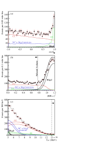
Figure  2.: The SNO spectrum vs $\cos\theta_{\odot}$, radial coordinate and recoil electron energy. Also shown is the MonteCarlo simulated events.

The NC events due to capture on deuteron has a peaked distribution around the energy of 6.25 MeV. These probability density functions are used to perform a maximum likelihood fit to the data.

2.3 Variations with time

SK already has enough statistics to divide their data into both energy and zenith angle bins. The latest SK data has been presented with a binning of eighth energy bins and each energy bin contains data subdivided into seven zenith angle bins.  [?]. This binning enables one to measure the day time and night time fluxes separately and study for any possible day/night asymmetry. Since in day time the neutrinos do not pass through the earths matter and in night time they traverse the earths matter an observed day/night asymmetry would be clear indicator of earths matter effect modifying the neutrino fluxes. The day/night asymmetry measured in SK and SNO are still not at a statistically significant level.

2.4 Evolution of the solar neutrino problem

Before the declaration of the SNO data there were two aspects of the solar neutrino problem. The first one is – in all the experiments the observed flux was less than SSM prediction. The second one was the ’problem of the ${}^{7}{Be}$ neutrinos’. We note that among the pre-SNO experiments SK and its predecessor Kamiokande is sensitive to the ${}^{8}{B}~{}$neutrinos. The ${}^{37}{Cl}$ experiment is sensitive mainly to the ${}^{8}{B}~{}$and ${}^{7}{Be}$ neutrinos while the sensitivity of the ${}^{71}{Ga}$ experiments amount to $pp$, ${}^{8}{B}~{}$and ${}^{7}{Be}$ neutrinos. Combining the ${}^{8}{B}$ flux measured in SK with the Cl data resulted in no room for the ${}^{7}{Be}$ neutrinos. Similarly the expected $pp$ flux in Ga consistent with solar luminosity plus the ${}^{8}{B}$ flux observed in SK indicated a negative flux of ${}^{7}{Be}$ neutrinos in Ga. The solar physics could not explain this preferential vanishing of ${}^{7}{Be}$ flux over ${}^{8}{B}~{}$flux as in the pp chain ${}^{7}{Be}$ comes before ${}^{8}{B}~{}$and any mechanism that reduces the ${}^{7}{Be}$ flux would eventually reduce the ${}^{8}{B}~{}$flux. Therefore the answer was sought in the properties of neutrinos and neutrino flavour conversion was considered as the most promising candidate for the solution. SNO provided the compelling evidence.

The SNO CC reaction is sensitive only to $\nu_{e}$ while the ES reaction in both SK and SNO is sensitive to both $\nu_{e}$ and $\nu_{\mu}/\nu_{\tau}$. Therefore a higher ES flux as compared to the CC flux will imply the presence of ${\nu_{\mu}}/{\nu_{\tau}}$ in the solar $\nu_{e}$ flux. Combining the SK ES and SNO CC results one gets

$$\phi_{ES}^{SK}-\phi_{CC}^{SNO}=0.57\pm 0.17\times 10^{6}{\rm/cm^{2}/sec}$$ (5)

This is a 3.3$\sigma$ signal for $\nu_{e}$ transition to an active flavour (or against $\nu_{e}$ transition to solely a sterile state).

The NC reaction is sensitive to all the three flavours with equal strength resulting in a greater sensitivity to the neutral current component in the solar $\nu_{e}$ flux. Comparing the NC and CC data from SNO one gets

$$\phi_{NC}^{SNO}-\phi_{CC}^{SNO}=3.41\pm 0.65\times 10^{6}{\rm/cm^{2}/sec}$$ (6)

In two circumstances we can have the CC and NC rates equal to each other. Either when there is no flavour conversion or for flavour conversion to a purely sterile state which does not interact with the detector. The observed CC/NC difference rules out both these possibilities at 5.3$\sigma$.

3. Two Flavour Oscillation

If neutrinos have mass then the flavour eigenstates ${\nu_{e}}$ and ${\nu_{\mu}}/{\nu_{\tau}}$ are different from the mass eigenstates $\nu_{1}$,$\nu_{2}$ and related as

$$\pmatrix{\nu_{e}\cr\nu_{x}}=\pmatrix{\cos\theta&\sin\theta\cr-\sin\theta&\cos\theta}\pmatrix{\nu_{1}\cr\nu_{2}}$$ (7)

where $\theta$ is the mixing angle in vacuum. This leads to neutrino oscillation in vacuum  [?]. Then the survival probability that a ${\nu_{e}}$ remains ${\nu_{e}}$ after traveling distance L in vacuum is

$$P_{\nu_{e}\nu_{e}}=1-\sin{{}^{2}}2\theta\sin{{}^{2}}(1.27{\Delta m}^{2}L/E)$$ (8)

$\Delta m^{2}=m_{2}^{2}-m_{1}^{2}$. The term containing $\Delta{m}^{2}$ is the oscillatory term resulting from coherent propagation of the mass eigenstates.

In matter, only $\nu_{e}$’s undergoes Charged current interaction giving rise to an matter induced mass term of the form $\sqrt{2}G_{F}N_{e}$. This changes the mixing angles as

$$\tan 2\theta_{M}=\frac{\Delta m^{2}\sin 2\theta}{\Delta m^{2}\cos 2\theta-2\sqrt{2}G_{F}n_{e}E}$$ (9)

$n_{e}$ is the electron density of the medium and $E$ is the neutrino energy. Eq. (9) demonstrates the resonant behavior of $\theta_{M}$. Assuming $\Delta m^{2}>0$ the mixing angle in matter is maximal (irrespective of the value of mixing angle in vacuum) for an electron density satisfying,

$$2\sqrt{2}G_{F}n_{e,res}E=\Delta m^{2}\cos 2\theta$$ (10)

This is the Mikheyev-Smirnov-Wolfenstein (MSW) effect of matter-enhanced resonant flavor conversion  [?].

The most general expression for $\nu_{e}$ survival probability in an unified formalism over the mass range $10^{-12}-10^{-3}$ eV² and for the mixing angle $\theta$ in the range [0,$\pi/2$] is  [?]

$$P_{ee} = P_{\odot}P_{\oplus}+(1-P_{\odot})(1-P_{\oplus})$$ (12)

$$+2\sqrt{P_{\odot}(1-P_{\odot})P_{\oplus}(1-P_{\oplus})}\cos\xi$$

where $P_{\odot}$ denotes the probability of conversion of $\nu_{e}$ to one of the mass eigenstates in the sun and $P_{\oplus}$ gives the conversion probability of the mass eigenstate back to the $\nu_{e}$ state in the earth. All the phases involved in the Sun, vacuum and inside Earth are included in $\xi$. Depending on the value of $\Delta m^{2}/E$ one has the following three limits
(i)in the regime $\Delta m^{2}/E\stackrel{{\scriptstyle<}}{{\sim}}5\times 10^{-10}$ eV²/MeV matter effects inside the Sun suppress flavor transitions while the effect of the phase $\xi$ remains. This is the vacuum oscillation limit.
(ii)For $\Delta m^{2}/E\stackrel{{\scriptstyle>}}{{\sim}}10^{-8}$ eV²/MeV, the total oscillation phase becomes very large and the $\cos\xi$ term in Eq. (12) averages out to zero signifying incoherent propagation of the neutrino mass eigenstates. This is the MSW limit.
(iii)For $5\times 10^{-10}$ eV²/MeV $\stackrel{{\scriptstyle<}}{{\sim}}\Delta m^{2}/E\stackrel{{\scriptstyle>}}{{\sim}}10^{-8}$ eV²/MeV, both matter effects inside the Sun and coherent oscillation effects in the vacuum become important. This is the quasi vacuum oscillation (QVO) regime.

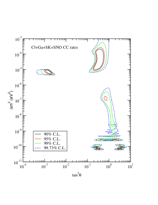
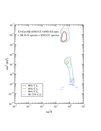
Figure  3.: The allowed regions in $\Delta{m}^{2}$ -$\tan^{2}\theta$ plane from data on total solar rates in the left panel and from data on total solar rates and SK spectrum data in right panel.

Next we present the results obtained by performing a $\chi^{2}$-analysis of the solar neutrino data. The procedure followed can be found in  [?,?,?]. In figure 3 we present the allowed regions obtained from analysis including the total fluxes measured in Cl, Ga, SK and SNO  [?]. There are basically five regions which are allowed – the small mixing angle region (SMA), the large mixing angle high $\Delta{m}^{2}$ regions (LMA), the large mixing angle-low $\Delta{m}^{2}$ regions (LOW), the vacuum oscillation regions symmetric about $\tan^{2}\theta=1.0$ and the quasi vacuum region between the LOW and the vacuum oscillation regions.

In the scond panel of figure 3 we present the allowed areas after including the SK spectrum data with the total rates data  [?]. The SMA region and large part of the vacuum oscillation region are seen to have been washed away with the inclusion of the SK spectrum data.

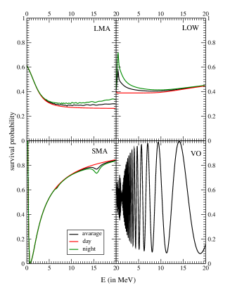
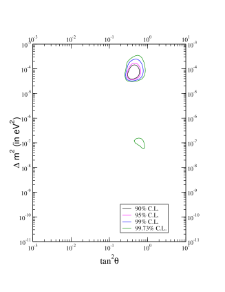
Figure  4.: The left panel shows the dependence of the probability on energy. The right panel gives the allowed area after including the latest SNO spectrum data including the NC events.

In the left panel of fig. 4 we show the dependence of the probabilities on energy. In the SMA and the VO oscillation regions the probability has a non-monotonic dependence on energy whereas in the LMA and LOW regions the survival probability does not have any appreciable dependence on energy beyond 5 MeV which is the threshold for SK and SNO. Thus these regions are favoured by the flat SK spectrum.

In the right panel of figure 4 ( from  [?]) we present the allowed regions obtained from an global $\chi^{2}$ analysis  [?,?,?,?] of the total rates observed in Cl and Ga (SAGE, GALLEX and GNO combined rate), the 1496 day SK zenith angle energy spectrum data and the recent SNO data of combined CC+ES+NC+background data in 17 day and 17 night energy bin. After the inclusion of the SNO results
(i) LMA emerges as the favoured solution.
(ii) The LOW region now appears only at 3$\sigma$.
(iii)Values of $\Delta m^{2}$ above $3\times 10^{-4}$ eV² are seen to be disfavored.
(iv)The QVO and VO solution are not allowed at $3\sigma$.
(v) Maximal mixing ($\theta=\pi/4$) is disfavored at $3.4\sigma$.
(vi) SMA solution is disfavored at 3.7$\sigma$
(vii)The Dark Side ($\theta>\pi/4$) solutions disappear.

Apart from including the SNO spectral data the figure 4 also has the new 1496 day SK zenith angle spectrum data. The data reveal a flat zenith angle spectrum. The inclusion of this data rule out the higher part of the LOW solution beyond $1.5\times 10^{-7}$ eV² for which peaks in the zenith-angle spectrum are expected  [?].

4. KamLAND

KamLAND is a 1000 ton liquid scintillator neutrino detector situated at the former site of Kamiokande  [?]. It looks for ${\bar{\nu_{e}}}$ oscillation coming from 16 reactors at distances 81 - 824 km. Most powerful reactors are at a distance $\sim$ 180 km. The detection process is $\bar{\nu_{e}}p\rightarrow e^{+}n$. The $e^{+}$ produced annihilates with the electrons in the medium to produce prompt photons. The neutrons get absorbed by the protons in the medium to produce delayed photons. The correlation of time,position and energy between these two constitute a grossly background free signal. The survival probability relevant in KamLAND is the vacuum survival probability (cf. eq. 8) summed over the distances from all the reactors. The average energy and length scales for KamLAND are $E_{\nu}\sim$ 3 MeV, L $\sim$ 1.8 $\times 10^{5}$ m which makes it sensitive to $\Delta m^{2}\sim 1.6\times 10^{-5}$ eV² which is in the LMA region. The figure 5 shows the probabilities for KamLAND for the average distance of 180 km and solar neutrinos for $\Delta{m}^{2}$ (=$6\times 10^{-5}$ eV²) and $\tan^{2}\theta$ (=0.5)  [?]. Whereas for the solar probabilities the $\Delta{m}^{2}$ dependence is completely averaged out in KamLAND the probability exhibits a $L/E$ dependence which gives it an unprecedented sensitivity to determine $\Delta{m}^{2}$ .

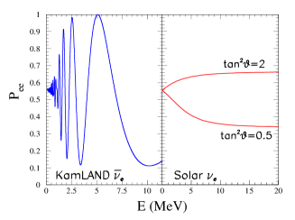
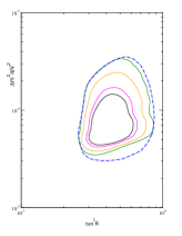
Figure  5.: The left figure shows the variation of the survival probability with energy for KamLAND and for the solar neutrinos. The right figure gives the allowed region from an analysis of KamLAND rate and global solar data. The allowed region from only solar analysis is shown also by the outer dashed line.

The solar best-fit predicts a rate in KamLAND $0.65^{+0.08}_{-0.39}$ (3$\sigma$)  [?] while the observed rate is $0.611\pm 0.094$ corresponding to 145 days of data. Thus KamLAND confirms the LMA solution. In figure 5 we show the allowed area obtained from a $\chi^{2}$-analysis of KamLAND rates data and global solar data  [?]. The contour obtained from only solar analysis is also drawn (dashed lines) for understanding the role played by KamLAND . The inclusion of the KamLAND rates data gives a lower bound of $\Delta m^{2}>4\times 10^{-5}$ eV². The other parts of the parameter space allowed from the solar analysis are not constrained much.

Figure 6 shows the allowed areas obtained from a $\chi^{2}$ analysis of the only KamLAND spectrum  [?]. For an average energy of 5 MeV and a distance 180 km a $\Delta{m}^{2}$ of $7\times 10^{-}5$ eV² corresponds to the oscillation wavelength ($\lambda$) $\sim$ the distance traveled(L) and $P_{ee}\approx 1$, for $\Delta{m}^{2}$ of $3.5\times 10^{-5}$ eV² $\lambda=2L$ and $P_{ee}=0.0$. Again for $\Delta{m}^{2}$ = $1.4\times 10^{-4}$ eV² $\lambda=L/2$ and $P_{ee}=1$. Since the KamLAND spectral data corresponds to a peak around 5 MeV islands around the first and the third $\Delta{m}^{2}$ are allowed whereas the middle $\Delta{m}^{2}$ is disfavoured as is seen from the panel 1 of figure 6.

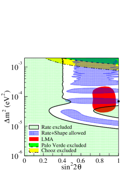
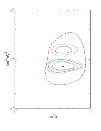
Figure  6.: The left panel shows the allowed regions in the $\mbox{$\Delta{m}^{2}$~{}}-\tan^{2}\theta$ plane from analysis of KamLAND spectrum data. The right panel shows the allowed region from a global analysis of KamLAND spectrum and solar neutrino data.

In the second panel of figure 6 we show the allowed area from KamLAND spectrum and global solar data obtained through a $\chi^{2}$ analysis  [?]. Inclusion of the KamLAND spectral data splits the allowed region into two zones at 99% C.L. low-LMA (LMA1) and high-LMA (LMA2). LMA2 has less statistical significance (by $\approx 2\sigma$) The global best-fit comes at $\Delta m^{2}=7.17\times 10^{-5}$ eV² and $\tan^{2}\theta=0.44$ in low-LMA. LOW region is disfavoured at $5\sigma$. Maximal mixing although allowed by the KamLAND spectrum data gets disfavoured at 3.4$\sigma$ by the overall analysis.

In the left panel of figure 7 we explore through a projected analysis of 1 kton year simulated spectrum the potential of KamLAND in distinguishing between the two allowed areas.

The allowed $\Delta m^{2}$ ranges around both low-LMA and high-LMA zones decrease in size. Since the solar data favours the low-LMA zone the allowed areas become more precise for spectrum simulated at the low-LMA zone while ambiguity between the two zones remains for high-LMA spectrum. In the right panel of 7 we show that a higher statistics (3 kton year) from KamLAND can remove this ambiguity almost completely determining $\Delta{m}^{2}$ to within 6%.

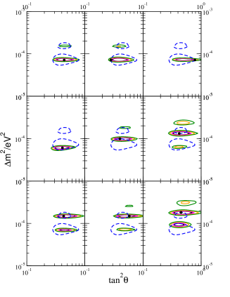
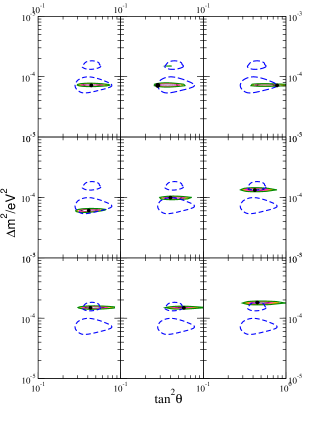
Figure  7.: The 1 kTy (left panel) and 3 kTy (right panel) projected contours of KamLAND and solar data. The points at which the spectra are simulated are shown by bold dots.

Analysis of solar and KamLAND data has been done in the realistic three neutrino scenario in  [?]. In this case the non-zero value of the mixing angle $\theta_{13}$ connecting the atmospheric sector and the solar sector modifies the allowed area in $\Delta m^{2}-\tan^{2}\theta$ parameter space. A third solution at a $\Delta{m}^{2}$ higher than the high-LMA zone gets marginally allowed for the three flavour case. As $\theta_{13}$ is increased the high-LMA zones tend to disappear.

5. Conclusions

The solar neutrino research began with a motivation of understanding the sun through the neutrino channel. Over the years it metamorphosed into a tool of unraveling the fundamental properties of the neutrinos. At the end of 2002 the status of the solar neutrino oscillation phenomenology can be summarised as
$\bullet$ Comparison of SNO CC and SNO NC signifies neutrino flavour conversion at $5.3\sigma$.
$\bullet$ Rules out transitions to pure sterile states at $5.3\sigma$.
$\bullet$ LMA is the favoured solution to the solar neutrino problem with $3\times 10^{-5}$ eV${}^{2}\leq\Delta m^{2}\leq 3\times 10^{-4}$ eV² and $0.25\leq\tan^{2}\theta\leq 0.87$ at $3\sigma$.
$\bullet$ KamLAND confirms LMA.
$\bullet$ Best-fit $\Delta m^{2}$ shifts from $6\times 10^{-5}$ eV² as obtained from global solar analysis to $7.2\times 10^{-5}$ eV².
$\bullet$ There is no significant change in best-fit $\theta$ ($\tan^{2}\theta=0.4$).
$\bullet$LMA region splits into two parts at 99% C.L..
$\bullet$$3\sigma$ allowed range after the first KamLAND data is $4.96\times 10^{-5}$ eV${}^{2}<\Delta m^{2}<2\times 10^{-4}$ eV² and $0.27<\tan^{2}\theta<0.88$.
$\bullet$Transitions to a mixed state is still allowed with $<13\%(52\%)$ sterile mixture at $1\sigma(3\sigma)$  [?].
At this juncture the emerging goals in solar neutrino research are
(i)precise determination of the oscillation parameters;
(ii)to observe the low energy end of the solar neutrino spectrum consisting of the pp,CNO and the ${}^{7}{Be}$ line and do a full solar neutrino spectroscopy.
As far as precision determination of $\Delta{m}^{2}$ is concerned KamLAND has remarkable sensitivity and 3 kton year KamLAND data can remove the ambiguity between the two presently allowed zones completely. Even before that a day-night asymmetry $>1$% in SNO can exclude LMA2  [?]. However the constraining power of KamLAND for $\theta$ is not as good being limited by the 6% systematic error and also by the fact that in the statistically significant regions the observed KamLAND spectrum corresponds to a peak in the survival probability where the $\theta$ sensitivity is very low. At the present value of the best-fit parameters in the low-LMA region a new KamLAND like reactor experiment with a baseline of $\sim$ 70 km will be sensitive to the the minimum in the survival probability increasing the $\theta$ sensitivity by a large amount  [?]. The upcoming Borexino experiment should see a rate $0.64\pm 0.03~{}(1\sigma)$ and no day-night asymmetry. It cannot differentiate between the two LMA regions. However it can provide a measurement of the ${}^{7}{Be}$ flux coming from the sun. Real time measurement of the $pp$ neutrino flux is the target of the so called ”LowNU” experiments like XMASS, HELLAZ, HERON. CLEAN, MUNU, GENIUS using $\nu-e$ scattering and LENS, MOON and SIREN using charged current reactions  [?]. All these experiments involve development of new and challenging experimental concepts and research work is in progress for evolving these techniques.

I acknowledge my collaborators A. Bandyopadhyay, S. Choubey, R. Gandhi and D.P. Roy.

REFERENCES

- [1] J. N. Bahcall, M.H. Pinsonneault and S. Basu, Astrophys. J. 555 (2001)990.
- [2] S. Goswami, arXiv:hep-ph/0303075
- [3] L. Miramonti and F. Reseghetti, Riv. Nuovo Cim. 25N7 (2002) 1 [arXiv:hep-ex/0302035].
- [4] B. T. Cleveland et al., Astroph. J. 496 (1998) 505.
- [5] J.N. Abdurashitov et al., (The SAGE collaboration), astro-ph/0204245; W. Hampel et al., (The Gallex collaboration), Phys. Lett. bf B447, 127 (1999); M. Altmann et al., (The GNO collaboration),Phys. Lett. B492,16 (2000).
- [6] Y. Fukuda et al., (The Kamiokande collaboration), Phys. Rev. Lett. 77, 1683 (1996).
- [7] S. Fukuda et al. [Super-Kamiokande Collaboration], Phys. Lett. B 539, 179 (2002).
- [8] Q.R. Ahmad et al., (The SNO Collaboration) Phys. Rev. Lett. 87, 071301 (2001).
- [9] Q. R. Ahmad et al. (SNO Collaboration),Phys. Rev. Lett. 89, 011301 (2002); Phys. Rev. Lett. 89, 011302 (2002).
- [10] S. Fukuda et al. [Super-Kamiokande Collaboration], Phys. Rev. Lett. 86 (2001) 5651.
- [11] M. B. Smy, hep-ex/0202020.
- [12] B. Pontecorvo, JETP 6, 429 (1958); Z. Maki, M. Nakagawa and S. Sakata, Prog. Theor. Phys. 28, 870 (1962).
- [13] L. Wolfenstein, Phys. Rev. D34, 969 (1986); S.P. Mikheyev and A.Yu. Smirnov, Sov. J. Nucl. Phys. 42(6), 913 (1985); Nuovo Cimento 9c, 17 (1986).
- [14] S.T. Petcov, Phys. Lett. B214 (1988) 139; Phys. Lett. B406, 355 (1997); G.L. Fogli, E.Lisi, D. Montanino and A. Palazzo, Phys. Rev. D62, 113004, (2000).
- [15] S. Choubey, S. Goswami and D. P. Roy, Phys. Rev. D 65, 073001 (2002) S. Choubey, S. Goswami, N. Gupta and D. P. Roy, Phys. Rev. D 64, 053002 (2001).
- [16] S. Choubey, S. Goswami, K. Kar, H. M. Antia and S. M. Chitre, Phys. Rev. D 64 (2001) 113001
- [17] A. Bandyopadhyay, S. Choubey, S. Goswami and K. Kar, Phys. Lett. B 519, 83 (2001).
- [18] S. Choubey, A. Bandyopadhyay, S. Goswami and D. P. Roy, arXiv:hep-ph/0209222.
- [19] A. Bandyopadhyay, S. Choubey, S. Goswami and D. P. Roy, Phys. Lett. B 540, 14 (2002).
- [20] A. Bandyopadhyay, S. Choubey and S. Goswami, Phys. Lett. B 555, 33 (2003).
- [21] V. Barger, D. Marfatia, K. Whisnant and B. P. Wood, Phys. Lett. B 537, 179 (2002); P. Creminelli, G. Signorelli and A. Strumia, [arXiv:hep-ph/0102234 (version 3)]; J. N. Bahcall, M. C. Gonzalez-Garcia and C. Pena-Garay, JHEP 0207, 054 (2002) ; P. C. de Holanda and A. Yu. Smirnov, arXiv:hep-ph/0205241; G. L. Fogli, E. Lisi, A. Marrone, D. Montanino and A. Palazzo, arXiv:hep-ph/0206162.
- [22] M. C. Gonzalez-Garcia, C. Pena-Garay and A. Yu. Smirnov, Phys. Rev. D 63, 113004 (2001).
- [23] K. Eguchi et al. [KamLAND Collaboration], Phys. Rev. Lett. 90, 021802 (2003).
- [24] J. N. Bahcall, M. C. Gonzalez-Garcia and C. Pena-Garay, arXiv:hep-ph/0212147.
- [25] A. Bandyopadhyay, S. Choubey, R. Gandhi, S. Goswami and D. P. Roy, arXiv:hep-ph/0211266.
- [26] A. Bandyopadhyay, S. Choubey, R. Gandhi, S. Goswami and D. P. Roy, arXiv:hep-ph/0212146.
- [27] G. L. Fogli, E. Lisi, A. Marrone, D. Montanino, A. Palazzo and A. M. Rotunno, arXiv:hep-ph/0212127;
- [28] P. C. de Holanda and A. Yu. Smirnov, arXiv:hep-ph/0212270.
- [29] A. Bandyopadhyay, S. Choubey and S. Goswami, arXiv:hep-ph/0302243, to appear in Phys. Rev.D.
- [30] The talk by S. Schönert, http://neutrino2002.ph.tum.de.