DESY 03–060

DFF 404/05/03

LPTHE–03–20

hep-ph/0307188

July 2003

Renormalisation group improved small-$\boldsymbol{x}$ Green’s function
M. Ciafaloni^(a), D. Colferai^(a), G.P. Salam^(b) and A.M. Staśto^(c)

^(a) Dipartimento di Fisica, Università di Firenze, 50019 Sesto Fiorentino (FI), Italy;
INFN Sezione di Firenze, 50019 Sesto Fiorentino (FI), Italy
^(b) LPTHE, Universities of Paris VI & VII and CNRS, 75252 Paris 75005, France
^(c) Theory Division, DESY, D22603 Hamburg;
H. Niewodniczański Institute of Nuclear Physics, Kraków, Poland

We investigate the basic features of the gluon density predicted by a renormalisation group improved small-$x$ equation which incorporates both the gluon splitting function at leading collinear level and the exact BFKL kernel at next-to-leading level. We provide resummed results for the Green’s function and its hard Pomeron exponent $\omega_{s}(\alpha_{s})$, and for the splitting function and its critical exponent $\omega_{c}(\alpha_{s})$. We find that non-linear resummation effects considerably extend the validity of the hard Pomeron regime by decreasing diffusion corrections to the Green’s function exponent and by slowing down the drift towards the non-perturbative Pomeron regime. As in previous analyses, the resummed exponents are reduced to phenomenologically interesting values. Furthermore, significant preasymptotic effects are observed. In particular, the resummed splitting function departs from the DGLAP result in the moderate small-$x$ region, showing a shallow dip followed by the expected power increase in the very small-$x$ region. Finally, we outline the extension of the resummation procedure to include the photon impact factors.

1 Introduction

Progress in understanding small-$x$ physics has been characterized by quite a number of steps: first the BFKL evolution equation [1] and its early prediction of the small-$x$ rise of hard cross sections, leading to the notion of hard Pomeron in perturbative QCD; then, the qualitative confirmation of such a rise at HERA [2], showing however a somewhat milder effect and, at the same time, good agreement with DGLAP evolution [3] at two-loop level; then the parallel calculation of the next-to-leading (NL) BFKL kernel [4, 5], leading to a dramatic decrease of the effect and to possible instabilities [6, 7, 8] of the leading $\log s$ series; finally, the proposal of various resummation approaches [9, 10, 11, 12, 13, 14, 15] and recipes to stabilize the series, in order to provide reliable predictions for processes with two hard scales and DIS-type processes.

The resummation approach proposed by some of us [9, 10, 11] and summarized in Sec. 2 identifies a few physical QCD effects that lead to large corrections. Firstly, the cross section dependence on the ratio of the hard scales of the problem, which is constrained by the renormalisation group (RG) requirement of single-logarithmic scaling violations in the relevant Bjorken variables. Secondly, the occurrence, at NL level, of the non-singular part (in moment space) of the anomalous dimension, yielding a sizable negative contribution. Finally, the running coupling effects which modify and make ambiguous the very notion of a hard Pomeron.

A key effect of the running coupling is that the BFKL evolution drifts towards smaller momentum scales, which are more strongly coupled, thus making non-perturbative physics more important at high energies. This means that the asymptotically leading Pomeron $\omega_{\mathbb{P}}$ [16] is actually a non-perturbative strong coupling quantity [17, 18]. This feature can be taken into account by the initial condition in the DGLAP evolution of structure functions, but may be a problem in the processes with two hard scales (like Mueller-Navelet jets [19], $\gamma^{*}\gamma^{*}$ scattering [20] etc.) where the perturbative hard Pomeron behavior can be observed at intermediate energies only.

Recently, it has been noticed that the transition to the Pomeron regime is driven, in some small-$x$ models, by a sudden tunneling effect [21, 22] at moderate values of $\alpha_{s}(t)\log 1/x$, so that the $b$-expansion [23] may be needed to suppress the Pomeron and to identify the hard Pomeron exponent $\omega_{s}(t)$ and its diffusion corrections [24, 25, 8, 26] (here $t=\log{\boldsymbol{k}}^{2}/\Lambda^{2}$, where ${\boldsymbol{k}}$ is the transverse momentum of the hard probe, and $\Lambda=\Lambda_{\mathrm{QCD}}$). Furthermore, the gluon splitting function is expected to be power behaved in the small-$x$ region too, but with a different exponent $\omega_{c}(t)$, due to running coupling effects. Therefore, in a resummed approach with running coupling one has to investigate various high-energy exponents: the hard Pomeron index $\omega_{s}(t)$ just mentioned, the resummed anomalous dimension singularity $\omega_{c}(t)$, which are generally different and perturbatively calculable, finally the asymptotic Pomeron $\omega_{\mathbb{P}}$ which is determined by the strong coupling behavior of the model.

The calculation of $\omega_{s}$ and $\omega_{c}$ was performed in the renormalisation group improved (RGI) approach of [11]. The result was that $\omega_{s}(t)$ carries important non-linear effects, leading to a stable and sizable decrease with respect to its LL BFKL value, and that $\omega_{c}(t)$ is sizably smaller than $\omega_{s}(t)$ also. However, the method of solution of the RGI equation used in [11] was best suited for the homogeneous equation, rather than the Green’s function (cfr. Sec. 2). Therefore, no real estimate of hard small-$x$ cross sections was really possible.

The purpose of the present paper is to further investigate the RGI approach by providing a numerical calculation in ${\boldsymbol{k}}$ and rapidity space of the Green’s function and of the corresponding splitting function. By then using ${\boldsymbol{k}}$-factorization [27] and the corresponding impact factors [28, 29, 30, 31], this sets the ground for a full cross section calculation. Here we also provide the high energy exponents and a semi-analytical treatment of the diffusion corrections. Part of the results of this paper have been summarized elsewhere [32].

In order to perform such an analysis, we introduce a resummation scheme slightly different from that proposed in [11], which turns out to be more convenient for numerical implementation, and belongs to a class of schemes that are identical modulo NNL$x$ (and NLO in $Q^{2}$) ambiguities intrinsic in the resummation approach. Recall, that — as summarized in the introductory Sec. 2 — the RGI approach incorporates leading and next-to-leading kernel information exactly, with some extra $\omega$-dependence ($\omega$ is the Mellin variable conjugated to $Y\sim\log 1/x$) so as to implement the RG constraints and the resummation of leading log collinear singularities mentioned before. Such requirements fix the form of the $\omega$-dependence of the kernel, apart from NNL terms, which remain and allow some freedom in the choice of the resummation scheme.

The exact definition of the kernel and of the resummation scheme is provided in Sec. 3. Stated in words, the main difference of the present formulation with respect to that of Ref. [11] is that the resummation of the collinear behavior quoted before is obtained here by the $\omega$-dependence of the leading kernel, rather than by a string of subleading ones. This allows us to include the full $\omega$-dependence of the one-loop anomalous dimension in a more direct way, while of course, leading plus NL kernel information is correctly incorporated, as in all such schemes.

The detailed investigation of the gluon Green’s function with its hard Pomeron behavior and its diffusion corrections is performed in Sec. 4, by analytical and numerical methods. The full numerical evaluation relies on the method introduced in Ref. [33]. Through the numerical study we are able to analyze the border between perturbative and non-perturbative Pomeron behavior, at realistic values of $Y$ and $\alpha_{s}$, and to extract the leading terms ($\sim bY$, $\sim b^{2}Y^{3}$) in the exponent of the perturbative part. Such terms can also be calculated analytically by the $b$-expansion method [24, 23]. We are thus able to identify both the hard Pomeron exponent at order ${\cal O}(b)$ and its diffusion corrections, and we notice sizable non-linear effects which stabilize the intercept, decrease the diffusion effects and slow down the drift towards the non-perturbative Pomeron regime.

We also provide in Sec. 5 the resummed splitting function. At the analytical level, we notice that the $\omega$-expansion method [10, 11] allows one to define a resummed characteristic function which, in the saddle-point approximation, can be related to the “duality” approach of Ref. [12], depending on the choice of the intercept in the latter. Beyond the saddle-point estimate, the resummed splitting function is evaluated numerically by the method of Ref. [34], and shows a power increase $\sim x^{-\omega_{c}(\alpha_{s})}$ in the very small-$x$ region, together with a shallow dip (compared to the DGLAP result) at moderately small $x$ values.

A preliminary discussion of the off-shell photon impact factors is provided in Sec. 6. Here we show how the resummation scheme incorporating collinear leading logs can be extended to the impact factor, and how the latter can be extracted from the result obtained in the recent literature [31]. We finally summarize and discuss our results in Sec. 7.

2 Renormalisation Group improved approach

The size of subleading corrections [4, 5] to the BFKL kernel ${\cal K}({\boldsymbol{k}},{\boldsymbol{k}}^{\prime})$ and the ensuing instabilities [6, 7, 8] make it mandatory to understand the physical origin of the large terms and possibly resum them. In a series of papers [9, 10, 11] (for a review see [35]) it was argued that most of the large corrections were due to collinear contributions, so as to achieve consistency of high-energy factorization [27] at subleading level [28] with the renormalisation group. This requires resummation [9] of both the energy scale-dependent terms of the kernel [5] and of the leading-log collinear logarithms [10] for both $Q\gg Q_{0}$ and $Q\ll Q_{0}$, with $Q$, $Q_{0}$ being the hard scales of the process. In the following we summarize the approach of [11], which incorporates both the renormalisation group requirements and the known exact forms of the leading [1] and next-to-leading [4, 5] BFKL kernel. A resummation for anomalous dimensions within a single collinear regime $Q\gg Q_{0}$ has been proposed in [12], and alternative resummations in [13, 14, 15].

2.1 ${\boldsymbol{k}}$-factorization and high-energy exponents

We consider a general process of scattering of two hard probes $A$ and $B$ with scales $Q$ and $Q_{0}$ at high center-of-mass energy $\sqrt{s}$. We assume that the cross section can be written in the following ${\boldsymbol{k}}$-factorized form [27]:

$$\sigma_{AB}(s;Q,Q_{0})=\int\frac{d\omega}{2\pi i}\,\frac{d^{2}{\boldsymbol{k}}}{{\boldsymbol{k}}^{2}}\,\frac{d^{2}{\boldsymbol{k}}_{0}}{{\boldsymbol{k}}_{0}^{2}}\left(\frac{s}{QQ_{0}}\right)^{\omega}h_{\omega}^{A}(Q,{\boldsymbol{k}})\;{\cal G}_{\omega}({\boldsymbol{k}},{\boldsymbol{k}}_{0})\;h_{\omega}^{B}(Q_{0},{\boldsymbol{k}}_{0})$$ (1)

where $h^{A}$ and $h^{B}$ are dimensionless impact factors which characterize the probes and ensure that $|{\boldsymbol{k}}|$ ($|{\boldsymbol{k}}_{0}|$) is of order $Q$ ($Q_{0}$), and the gluon Green’s function is defined by

$${\cal G}_{\omega}({\boldsymbol{k}},{\boldsymbol{k}}_{0})=\langle{\boldsymbol{k}}|[\omega-{\cal K}_{\omega}]^{-1}|{\boldsymbol{k}}_{0}\rangle\;.$$ (2)

The function ${\cal K}_{\omega}$ is the kernel of the small-$x$ equation of the general form

$$\omega{\cal G}_{\omega}({\boldsymbol{k}},{\boldsymbol{k}}_{0})=\delta^{2}({\boldsymbol{k}}-{\boldsymbol{k}}_{0})+\int\frac{d^{2}{\boldsymbol{k}}^{\prime}}{\pi}\;{\cal K}_{\omega}({\boldsymbol{k}},{\boldsymbol{k}}^{\prime})\;{\cal G}_{\omega}({\boldsymbol{k}}^{\prime},{\boldsymbol{k}}_{0})\;.$$ (3)

The factorization formula (1) involving two-(Regge)gluon exchange, has been justified up to NL $\log s$ level in Refs. [28] for initial partons and in [29, 30] for physical probes. At further subleading levels, many (Regge)gluon Green’s functions contribute to the cross section as well, due to the s-channel iteration. However, our purpose here is to incorporate leading-twist collinear behavior, and at that level the two-gluon contribution is dominant, so that we shall consider only the contribution (1) in the following.

While ${\boldsymbol{k}}$-factorization is supposed to be valid for $\alpha_{s}\lesssim\omega\ll 1$, we shall sometimes extrapolate Eq. (1) to sizable values of $\omega={\cal O}(1)$ and moderate values of $s$, encouraged by the stability of our resummation, and by the possibility of incorporating phase space thresholds in Eq. (1) (cfr. Sec. 6). It should be kept in mind that such a region lies outside the validity range of Eq. (1), so that the extrapolated Green’s function loses — most probably — its original meaning as two-(Regge)gluon propagator.

In writing Eq. (1), we have performed the choice of energy scale $s_{0}=QQ_{0}$, in terms of which the high energy kinematics shows a simpler phase space, as explained in more detail in Sec. 6. Actually, for intermediate subenergies it is more convenient to introduce as energy variables the scalar products of type $\nu=2k_{\mu}k_{0}^{\mu}$, which have $|{\boldsymbol{k}}||{\boldsymbol{k}}_{0}|$ as threshold, so that $|{\boldsymbol{k}}||{\boldsymbol{k}}_{0}|/\nu$ is a good Mellin variable. Correspondingly, the energy dependence of the Green’s function and of the impact factors is defined by ($k\equiv|{\boldsymbol{k}}|,k_{0}\equiv|{\boldsymbol{k}}_{0}|$)

$${\cal G}(\nu,{\boldsymbol{k}},{\boldsymbol{k}}_{0}) =\int\frac{d\omega}{2\pi i}\left(\frac{\nu}{kk_{0}}\right)^{\omega}{\cal G}_{\omega}({\boldsymbol{k}},{\boldsymbol{k}}_{0})$$ (4)

$$\equiv\frac{1}{kk_{0}}G(Y;t,t_{0})\;,\qquad\left(Y\equiv\log\frac{\nu}{kk_{0}}\;,\qquad t\equiv\log\frac{k^{2}}{\Lambda^{2}}\right)$$

and

$$h(\nu,Q,{\boldsymbol{k}})=\int\frac{d\omega}{2\pi i}\left(\frac{\nu}{Qk}\right)^{\omega}h_{\omega}(Q,{\boldsymbol{k}})\;.$$ (5)

In this paper, we are mostly interested in the properties of the two-scale Green’s function and of its high-energy exponents. It was pointed out in [11] that, in the improved approach with running coupling, the high energy limits of the Green’s function and of the collinear splitting functions are regulated by different indices, which both originate from the frozen coupling hard Pomeron exponent. We shall define the index $\omega_{s}(t)$ by (cfr. Sec. 4.4)

$$G(Y;t,t_{0})\simeq\frac{1}{\sqrt{2\pi\bar{\alpha}_{s}\chi^{\prime\prime}Y}}\exp[\omega_{s}(\frac{t+t_{0}}{2})Y+\text{diffusion corrections}]\;,\qquad\bar{\alpha}_{s}\equiv\alpha_{s}\frac{N_{c}}{\pi}$$ (6)

in the limit $\omega_{s}(t)Y\gg 1$ and $t\simeq t_{0}\gg 1$, and the index $\omega_{c}(t)$ by

$$xP(\bar{\alpha}_{s}(k^{2}),x)\;\stackrel{{\scriptstyle x\rightarrow 0}}{{\longrightarrow}}\;x^{-\omega_{c}(t)}p(\bar{\alpha}_{s})\;,$$ (7)

where $P(\bar{\alpha}_{s}(k^{2}),x)$ is the resummed gluon-gluon splitting function (Sec. 5). The exponent $\omega_{s}$ in Eq. (6) used to be defined as the location of the anomalous dimension singularity in the saddle point approximation. It is now understood [11], see also [13], that this singularity is actually an artefact of the saddle point approximation, and that the true anomalous dimension singularity, located at $\omega=\omega_{c}(t)$, causes the power behavior of the effective splitting function. This result has then been confirmed in the alternative resummation procedures of [36, 37, 13].

Even the definition in Eq. (6) is not free of ambiguities, due to the occurrence of diffusion corrections to the exponent [24, 25, 8, 26] which rapidly increase with $Y$, and to the contamination of the non-perturbative Pomeron, which dominates above some critical rapidity [22, 23].

In the following, both regimes $t\simeq t_{0}$ and $t\gg t_{0}$ will be discussed in detail in the RG-improved approach, by emphasizing our perturbative predictions and their range of validity.

2.2 Scale changing transformations

Let us note that the symmetrical scale choice $\nu_{0}=kk_{0}$ performed in Eq. (4) is not the only possible one, and is physically justified only in the case $k\sim k_{0}$. This configuration occurs for example in the process of $\gamma^{*}\gamma^{*}$ scattering at high energy with comparable virtualities of both photons [20], forward jet/$\pi^{0}$ production in DIS [38] or production of 2 hard jets at hadron colliders [19]. However, in the typical deep inelastic situation, when one of the scales is much larger, $k\gg k_{0}$ ($k_{0}\gg k$) the correct Bjorken variable is rather $k^{2}/s$ ($k_{0}^{2}/s$). In order to switch to this asymmetric case one should perform a similarity transformation on the gluon Green’s function of the form

$${\cal G}_{\omega}\rightarrow\bigg{(}{k_{>}\over k_{<}}\bigg{)}^{\omega}{\cal G}_{\omega}\;,$$ (8)

where $k_{>}=\max(k,k_{0})$ and $k_{<}=\min(k,k_{0})$. The transformation (8) implies the following change of kernel ${\cal K}_{\omega}$

$${\cal K}_{\omega}(k,k^{\prime}) \;\rightarrow\;{\cal K}^{u}_{\omega}(k,k^{\prime})\,=\,{\cal K}_{\omega}(k,k^{\prime})\bigg{(}{k\over k^{\prime}}\bigg{)}^{\omega}\;,\qquad\nu_{0}=k^{2}\;,$$ (9a)

$${\cal K}_{\omega}(k,k^{\prime}) \;\rightarrow\;{\cal K}^{l}_{\omega}(k,k^{\prime})\,=\,{\cal K}_{\omega}(k,k^{\prime})\bigg{(}{k^{\prime}\over k}\bigg{)}^{\omega}\;,\qquad\nu_{0}=k^{\prime}{}^{2}\;,$$ (9b)

where now ${\cal K}^{u}_{\omega}$ (${\cal K}^{l}_{\omega}$) means the kernel for the upper-$k^{2}$ (lower-$k^{\prime}{}^{2}$) energy scale choice.

Our goal is to find a resummed prescription for ${\cal K}_{\omega}(k,k^{\prime})$ which takes into account the large $Y$ terms and is consistent with renormalisation group equations. The kernel ${\cal K}_{\omega}(k,k^{\prime})$ is not scale invariant, and it can be expanded in powers of the coupling constant as follows

$${\cal K}_{\omega}(k,k^{\prime})=\sum_{n=0}^{\infty}[\bar{\alpha}_{s}(k^{2})]^{n+1}\;{\cal K}_{n}^{\omega}(k,k^{\prime})\;.$$ (10)

where

$$\bar{\alpha}_{s}(k^{2})={1\over b\log(k^{2}/\Lambda^{2})}\;,\qquad b={11\over 12}-{N_{f}\over 6N_{c}}\;,$$ (11)

and the coefficient kernels ${\cal K}_{n}^{\omega}(k,k^{\prime})$ are now scale invariant, and additionally carry some $\omega$-dependence. We shall now see how the renormalisation group constraints on ${\cal K}_{\omega}^{u}$ and ${\cal K}_{\omega}^{l}$ determine the collinear behavior of ${\cal K}_{\omega}$ .

2.3 Renormalisation group constraints and shift of $\gamma$ poles

It is important to notice that the $\omega$-dependence of the scale invariant kernels ${\cal K}_{n}^{\omega}$, present in Eq. (10), is not negligible (even for the small $\omega$ values being considered) and follows from the requirement that collinear singularities have to be single logarithmic in both regimes $k\gg k_{0}$ and $k_{0}\gg k$. If $k\gg k_{0}$, it is simplest to discuss the kernel in its form ${\cal K}_{\omega}^{u}$, Eq. (9a). A leading-$\log k^{2}$ analysis for $k\gg k^{\prime}$ shows that its collinear singularities are determined by the non-singular part (in $\omega$ space), $A_{1}(\omega)$, of the gluon anomalous dimension,

$$\bar{\alpha}_{s}A_{1}(\omega)=\gamma_{gg}(\omega)-{\bar{\alpha}_{s}\over\omega},$$ (12)

and

$$A_{1}(\omega)=-{11\over 12}+{\cal O}(\omega),\hskip 28.45274pt(N_{f}=0)\;,$$ (13)

In contrast the singular part $\bar{\alpha}_{s}/\omega$ is accounted for by the iteration of the BFKL equation itself.

To be precise, one has

$${\cal K}_{\omega}^{u}(k,k^{\prime})\simeq\frac{\bar{\alpha}_{s}(k^{2})}{k^{2}}\exp\int_{t^{\prime}}^{t}d(\log\kappa^{2})\;A_{1}(\omega)\bar{\alpha}_{s}(\kappa^{2})=\frac{\bar{\alpha}_{s}(k^{2})}{k^{2}}\left(1-b\bar{\alpha}_{s}(k^{2})\log\frac{k^{2}}{k^{\prime}{}^{2}}\right)^{-\frac{A_{1}(\omega)}{b}}\;,$$ (14)

where $t=\log k^{2}/\Lambda_{QCD}^{2}$, indeed showing single logarithmic scaling violations. A similar reasoning, yields the collinear behavior of ${\cal K}_{\omega}^{l}$ from Eq. (9b) with the opposite strong ordering behavior $k^{\prime}\gg k$, which is relevant in the regime $k_{0}\gg k$.

But ${\cal K}_{\omega}^{u}$ and ${\cal K}_{\omega}^{l}$ are related to ${\cal K}_{\omega}$ by the $\omega$-dependent similarity transformations (9a,9b), so that the latter must have the following collinear structure

$${\cal K}_{\omega}(k,k^{\prime})\simeq\bar{\alpha}_{s}(k^{2})\left[\frac{1}{k^{2}}\left(\frac{k^{\prime}}{k}\right)^{\omega}\left(\frac{\bar{\alpha}_{s}(k^{2})}{\bar{\alpha}_{s}(k^{\prime}{}^{2})}\right)^{-\frac{A_{1}(\omega)}{b}}\Theta(k-k^{\prime})\;+\right.\\ \left.+\;\frac{1}{k^{\prime}{}^{2}}\left(\frac{k}{k^{\prime}}\right)^{\omega}\left(\frac{\bar{\alpha}_{s}(k^{2})}{\bar{\alpha}_{s}(k^{\prime}{}^{2})}\right)^{\frac{A_{1}(\omega)}{b}-1}\Theta(k^{\prime}-k)\right]\,.$$ (15)

In this expression one can see that the $\omega$-dependence provided by $\left(\frac{k_{<}}{k_{>}}\right)^{\omega}$ is essential, because $k_{>}/k_{<}$ can be a large parameter. We also keep the $\omega$-dependence in $A_{1}(\omega)$, in order to take into account the full one-loop anomalous dimension.

By expanding in $b\bar{\alpha}_{s}$ the renormalisation group logarithms present in the collinear behavior of Eqs. (14,15), we obtain the leading collinear singularities of the coefficient kernels ${\cal K}^{\omega}_{n}$ in Eq. (10). This implies that, in $\gamma$-space, the corresponding eigenvalues have the following structure

$$\chi_{n}^{\omega}(\gamma)={1\!\cdot\!A_{1}(A_{1}+b)\cdots[A_{1}+(n-1)b]\over(\gamma+\frac{\omega}{2})^{n+1}}+{1\!\cdot\!(A_{1}-b)A_{1}\cdots[A_{1}-nb]\over(1-\gamma+\frac{\omega}{2})^{n+1}}\;,$$ (16)

where the $\omega$ dependence of $A_{1}$ is left implicit. Therefore the position of the $\gamma\rightarrow 0$ ($\gamma\rightarrow 1$) poles is shifted by $-{\textstyle\frac{\omega}{2}}$ ($+{\textstyle\frac{\omega}{2}}$) for the kernel (15) with symmetrical scale choice $\nu_{0}=kk_{0}$. Through this shift one is able to resum [9] the higher order $\gamma$-poles of the kernel that are due to scale changing effects.

In fact, the leading and next-to-leading eigenvalues corresponding to this symmetrical choice of scale have the collinear behavior

$$\chi_{0}^{\omega}(\gamma)\simeq{1\over\gamma+{\textstyle\frac{\omega}{2}}}+{1\over 1-\gamma+{\textstyle\frac{\omega}{2}}}\;,$$

$$\chi_{1}^{\omega}(\gamma)\simeq{A_{1}(\omega)\over(\gamma+{\textstyle\frac{\omega}{2}})^{2}}+{A_{1}(\omega)-b\over(1-\gamma+{\textstyle\frac{\omega}{2}})^{2}}\;.$$ (17)

Now, in order to obtain the NLL coefficient [11] in the $\bar{\alpha}_{s}$ expansion one has to expand in $\omega$ the term $\chi_{0}^{\omega}(\gamma)$ to first order with subsequent identification $\omega\rightarrow\bar{\alpha}_{s}\chi_{0}^{\omega=0}$, and add the $\chi_{1}^{\omega=0}$ terms. The result for the NLL eigenvalue in the collinear approximation then reads

$$\chi_{1}^{\mathrm{coll}}(\gamma)=\left[\bar{\alpha}_{s}\chi_{0}^{\omega}(\gamma){\partial\chi_{0}^{\omega}\over\partial\omega}+\chi_{1}^{\omega}\right]_{\omega=0}=-{1\over 2\gamma^{3}}-{1\over 2(1-\gamma)^{3}}+{A_{1}(0)\over\gamma^{2}}+{A_{1}(0)-b\over(1-\gamma)^{2}}+\dots\;.$$ (18)

We note that the $\omega$-dependent shift has generated cubic poles $\frac{1}{\gamma^{3}},\frac{1}{(1-\gamma)^{3}}$ which seem to imply double logs $\log^{2}\frac{k_{<}^{2}}{k_{>}^{2}}$, but are actually needed with the choice of scale $kk_{0}$ in order to recover the correct Bjorken variable $k_{>}^{2}/s$. The collinear terms with $A_{1}(\omega)$ have instead generated double poles $\frac{1}{\gamma^{2}},\frac{1}{(1-\gamma)^{2}}$ which correspond to single logs, $\log\frac{k_{<}^{2}}{k_{>}^{2}}$.

The double and cubic poles at $\gamma=0$ and $\gamma=1$ so obtained are precisely those of the full NLL BFKL kernel eigenvalue. In fact Eq. (18) is a collinear approximation to the full NLL BFKL kernel eigenvalue [4, 5] which has the following form

$$\chi_{1}(\gamma) =-\frac{b}{2}[\chi^{2}_{0}(\gamma)+\chi^{\prime}_{0}(\gamma)]-\frac{1}{4}\chi_{0}^{\prime\prime}(\gamma)-\frac{1}{4}\left(\frac{\pi}{\sin\pi\gamma}\right)^{2}\frac{\cos\pi\gamma}{3(1-2\gamma)}\left(11+\frac{\gamma(1-\gamma)}{(1+2\gamma)(3-2\gamma)}\right)$$

$$\quad+\left(\frac{67}{36}-\frac{\pi^{2}}{12}\right)\chi_{0}(\gamma)+\frac{3}{2}\zeta(3)+\frac{\pi^{3}}{4\sin\pi\gamma}$$

$$\quad-\sum_{n=0}^{\infty}(-1)^{n}\left[\frac{\psi(n+1+\gamma)-\psi(1)}{(n+\gamma)^{2}}+\frac{\psi(n+2-\gamma)-\psi(1)}{(n+1-\gamma)^{2}}\right]\;.$$ (19)

It turns out that the collinear approximation (18) above reproduces the exact eigenvalue (19) up to 7% [11, 35] accuracy when $\gamma\in]0,1[$. This suggests that the collinear terms are the dominant contributions in the NLL kernel.

In the following, we shall normally incorporate the shift of $\gamma$-poles in the form

$$\chi_{n}^{\omega}(\gamma)=\chi_{nL}^{\omega}(\gamma+{\textstyle\frac{\omega}{2}})+\chi_{nR}^{\omega}(1-\gamma+{\textstyle\frac{\omega}{2}})\;,$$ (20)

where $\chi_{nL}^{\omega}$ ($\chi_{nR}^{\omega}$) have only $\gamma\rightarrow-{\textstyle\frac{\omega}{2}}$ ($\gamma\rightarrow 1+{\textstyle\frac{\omega}{2}}$) singularities of the type in Eq. (16). In this way the collinear singularities are single logarithmic in both limits $k\gg k_{0}$ and $k_{0}\gg k$, and the energy scale dependent terms are automatically resummed. The modified leading-order eigenvalue that we adopt has the following structure (compare (17)):

$$\chi_{0}^{\omega}=2\psi(1)-\psi(\gamma+{\textstyle\frac{\omega}{2}})-\psi(1-\gamma+{\textstyle\frac{\omega}{2}})\;,$$ (21)

in the case of symmetric choice of energy scale $\nu_{0}=kk_{0}$. This form of the kernel was considered previously in [39, 40]. It is obtained from the leading order BFKL kernel by imposing the so-called kinematical (or consistency) constraint [41, 42, 43] which limits the virtualities of the transverse momenta of the gluons in the real emission part of the kernel. The origin of this constraint is the requirement that in the multi-Regge kinematics the virtualities of the exchanged gluons be dominated by their transverse parts. The NLL contribution of the resummed kernel, $\chi_{1}^{\omega}$ was then [11] constructed by the requirement that the collinear limit in Eq. (17) should be correctly reproduced, and the exact form of the NL kernel (19) should be obtained also.

The final NLL eigenvalue function proposed in [10, 11] reads

$$\chi_{1}^{\omega}(\gamma) = \chi_{1}(\gamma)+{1\over 2}\chi_{0}(\gamma){\pi^{2}\over\sin^{2}\pi\gamma}$$ (22)

$$-A_{1}(0)\psi^{\prime}(\gamma)-[A_{1}(0)-b]\psi^{\prime}(1-\gamma)$$

$$+A_{1}(\omega)\psi^{\prime}(\gamma+{\textstyle\frac{\omega}{2}})+[A_{1}(\omega)-b]\psi^{\prime}(1-\gamma+{\textstyle\frac{\omega}{2}})$$

$$-{\pi^{2}\over 6}[\chi_{0}(\gamma)-\chi_{0}^{\omega}(\gamma)]\;.$$

The first line is the original NLL term $\chi_{1}(\gamma)$ with the subtraction of the cubic poles which come from the changes of the energy scale and which are resummed by the leading order $\omega$-dependent kernel (21). The second and third lines contain shifted collinear double poles, and finally the last line contains the shifted single poles which additionally appear as an artefact of the resummation procedure.

2.4 $\boldsymbol{\omega}$-expansion and collinear resummation

In the present paper we choose a form of the improved kernel that differs somewhat from that of Ref. [11] — quoted in Eqs. (21,22) — by using the possibility of translating part of the $\alpha_{s}$-dependence in Eq. (10) into additional $\omega$-dependence. Actually, it was pointed out in [10, 11] that, at high energies, $\omega$ is a more useful expansion parameter than $\alpha_{s}(k^{2})$, the relation being given roughly by $\omega\simeq\bar{\alpha}_{s}\chi_{0}$, as noticed already in connection with Eq. (18).

The $\omega$-expansion is a systematic way of solving the homogeneous equation

$$(\omega-{{\cal K}_{\omega}}){\cal F}_{\omega}(k)=0\;,$$ (23)

where ${\cal K}_{\omega}$ is given by Eq. (10), by the $\gamma$-representation

$${\cal F}_{\omega}(t)=\int\frac{d\gamma}{2\pi i}\;e^{\gamma t-\frac{1}{b\omega}X_{\omega}(\gamma)}\;,$$ (24)

in which $\chi_{\omega}(\gamma)=X^{\prime}_{\omega}(\gamma)$ satisfies a non-linear integro-differential equation equivalent to Eq. (23). The latter is derived by using the representation $t\to-\partial_{\gamma}$ in Eq. (10), and is given by [11]

$$\chi_{\omega}(\gamma)=\chi^{\omega}_{0}(\gamma)+\left(\frac{\omega}{\chi_{\omega}-b\omega\partial_{\gamma}}\right)\chi^{\omega}_{1}+\left(\frac{\omega}{\chi_{\omega}-b\omega\partial_{\gamma}}\right)^{2}\chi^{\omega}_{2}+\cdots\;.$$ (25)

Approximate solutions to Eq. (25) can be obtained either by truncating at, say, NL level (i.e., setting $\chi_{2}=\chi_{3}=\cdots=0$), or by expanding in the $\omega$-parameter to all orders. The latter procedure yields the solution [10, 11]

$$\chi_{\omega}(\gamma)=\chi_{0}^{\omega}(\gamma)+\omega\frac{\chi_{1}^{\omega}(\gamma)}{\chi_{0}^{\omega}(\gamma)}+\omega^{2}\frac{1}{\chi_{0}^{\omega}(\gamma)}\left[\frac{\chi_{2}^{\omega}(\gamma)}{\chi_{0}^{\omega}(\gamma)}+b\left(\frac{\chi_{1}^{\omega}}{\chi_{0}^{\omega}}\right)^{\prime}-\left(\frac{\chi_{1}^{\omega}}{\chi_{0}^{\omega}}\right)^{2}\right]+\dots\;,$$ (26)

and amounts to replacing the kernel ${\cal K}_{\omega}$ by an effective kernel $\bar{\alpha}_{s}(k^{2}){\cal K}_{\omega}^{{\mathrm{eff}}}$, where ${\cal K}_{\omega}^{{\mathrm{eff}}}$ is scale invariant. The corresponding characteristic function $\chi_{\omega}(\gamma)$ in Eq. (26) is — very roughly — obtained by the replacement $\bar{\alpha}_{s}\rightarrow\omega/\chi_{\omega}$ in Eq. (10), so that indeed $\omega$ plays the role of a new expansion parameter. A virtue of the expansion (26) is that it contains simple (leading) collinear poles only, because the double-poles left in $\chi_{1}^{\omega}$ after the $\omega$-shift are canceled by the denominators.

The $\omega$-expansion is particularly useful for the resummation of the leading collinear singularities of Eqs. (15) and (16). Suppose we first take $\bar{\alpha}_{s}$ frozen (limit $b=0$). Then, the leading poles of Eq. (16) have approximately the factorized form

$$\chi_{n}^{\omega}\simeq\chi_{0}^{\omega}(\chi_{{\mathrm{c}}}^{\omega})^{n}\;,\qquad\chi_{{\mathrm{c}}}^{\omega}=\frac{A_{1}(\omega)}{\gamma+{\textstyle\frac{\omega}{2}}}+\frac{A_{1}(\omega)}{1-\gamma+{\textstyle\frac{\omega}{2}}}\;,$$ (27)

(valid for $\gamma+{\textstyle\frac{\omega}{2}}\simeq 0$ or $1-\gamma+{\textstyle\frac{\omega}{2}}\simeq 0$), so that the resummed behavior (15) reads

$${\cal K}_{\omega}\simeq\sum_{n=0}^{\infty}\bar{\alpha}_{s}K_{0}^{\omega}[\bar{\alpha}_{s}K_{{\mathrm{c}}}^{\omega}]^{n}=\bar{\alpha}_{s}K_{0}^{\omega}(1-\bar{\alpha}_{s}K_{{\mathrm{c}}}^{\omega})^{-1}\;.$$ (28)

Exactly the same result can be obtained by the $\omega$-expansion (26) truncated at the NL level, by setting $\chi_{1}^{\omega}/\chi_{0}^{\omega}\simeq\chi_{{\mathrm{c}}}^{\omega}$, and thus considering the kernel

$$\tilde{\cal K}_{\omega}=\bar{\alpha}_{s}(K^{\omega}_{0}+\omega K^{\omega}_{\mathrm{c}})\;.$$ (29)

In fact, the resolvent of the latter is given by

$$\tilde{{\cal G}}_{\omega}\equiv[\omega-\tilde{\cal K}_{\omega}]^{-1}\simeq(1-\bar{\alpha}_{s}K^{\omega}_{\mathrm{c}})^{-1}\left[\omega-\bar{\alpha}_{s}K^{\omega}_{0}(1-\bar{\alpha}_{s}K^{\omega}_{\mathrm{c}})^{-1}\right]^{-1}\;,$$ (30)

and is then proportional to the Green’s function of the resummed kernel (28).

In other words, leading-log collinear singularities are equivalently incorporated by a string of subleading kernels (as in Eq. (28)), or by a NL contribution of order $\bar{\alpha}_{s}\omega$ (as in Eq. (29)) — apart from a redefinition of the impact factors. In the realistic case with running coupling it is straightforward to check that $b$-dependence only remains in the first term of the $\omega$-expansion (26)

$$\chi_{\omega}(\gamma)\simeq\chi_{0}^{\omega}+\omega\left(\frac{A_{1}}{\gamma+{\textstyle\frac{\omega}{2}}}+\frac{A_{1}-b}{1-\gamma+{\textstyle\frac{\omega}{2}}}\right)+\dots\;,$$ (31)

whereas it cancels out in all remaining subleading terms. Therefore, in order to incorporate the leading log collinear behavior in the form (31) we can set, for instance,

$$\tilde{\cal K}_{\omega}=\bar{\alpha}_{s}(\boldsymbol{q}^{2})K^{\omega}_{0}+\omega\bar{\alpha}_{s}(k_{>}^{2})K^{\omega}_{\mathrm{c}}+\mathrm{NLL}\;,$$ (32)

as an improved leading kernel. Here we assume that the scale for $\bar{\alpha}_{s}$ in the leading BFKL part is provided by the momentum of the emitted gluon $\boldsymbol{q}={\boldsymbol{k}}-{\boldsymbol{k}}^{\prime}$, as suggested by the $b$-dependent part of the NLL eigenvalue in Eq. (19), which corresponds to the kernel $b\frac{1}{\boldsymbol{q}^{2}}\log\frac{\boldsymbol{q}^{2}}{{\boldsymbol{k}}^{2}}\big{|}_{\mathrm{Reg}}$ (see [5]), and — via $\omega$-expansion — to the $b$-term in Eq. (31). A simplified version of Eq. (32) without the NLL term and with one collinear term (for $\gamma\rightarrow 0$) was used in [43] for a phenomenological analysis of the structure functions.

Note that, if we take literally the $\omega$-expansion (26) with the choice of NLL term (22), then $\chi_{1}^{\omega}/\chi_{0}^{\omega}$ would coincide with $\chi_{{\mathrm{c}}}^{\omega}$ close to the collinear poles, but would be different in detail away from them, and would actually contain spurious poles at complex values of $\gamma$ due to the zeroes of $\chi_{0}^{\omega}(\gamma)$. Such poles cancel out if the full $\omega$-expansion series (26) is summed up, but are present at any finite truncation of the series, thus implying poor convergence of the solution whenever $\gamma$-values close to the spurious poles become important. For this reason in this paper we prefer to resum collinear singularities by the improved kernel (32), which contains only collinear poles. Furthermore, the NLL term needed to complete Eq. (32) — to be detailed in the next section — turns out to have only simple (leading) collinear poles, because the running coupling terms have been already included in the $q^{2}$-scale dependence of the running coupling. Therefore, the full kernel has the same virtues as Eq. (26) in the collinear limit and, lacking spurious poles, is more suitable for numerical iteration.

3 Form of the resummed kernel

3.1 Next-to-leading coefficient kernel

We have still to incorporate in our improved kernel the exact form of the NLL result [4, 5] in the scheme of the $\bar{\alpha}_{s}$ expansion, i.e. (32). We choose to start from the leading kernel in Eq. (32) which incorporates both the collinear resummation and the running coupling effects due to the choice of scale $\boldsymbol{q}^{2}$. The full improved kernel then has the form

$$\tilde{\cal K}_{\omega}=\bar{\alpha}_{s}(\boldsymbol{q}^{2})K^{\omega}_{0}+\omega\bar{\alpha}_{s}(k_{>}^{2})K^{\omega}_{\mathrm{c}}+\bar{\alpha}_{s}^{2}(k_{>}^{2})\tilde{K}^{\omega}_{1}\;,$$ (33)

where $k_{>}=\max(k,k^{\prime})$, $k_{<}=\min(k,k^{\prime})$, and $\tilde{K}^{\omega}_{1}$ is determined below.

We recall that the Mellin transform of the collinear part ${\cal K}_{{\mathrm{c}}}^{\omega}$, defined by

$$\chi_{{\mathrm{c}}}^{\omega}(\gamma)={A_{1}(\omega)\over\gamma+{\textstyle\frac{\omega}{2}}}+{A_{1}(\omega)\over 1-\gamma+{\textstyle\frac{\omega}{2}}}\;,$$ (34)

leads to the expression

$$K_{{\mathrm{c}}}^{\omega}(k,k^{\prime})=\frac{A_{1}(\omega)}{k_{>}^{2}}\left(\frac{k_{<}}{k_{>}}\right)^{\omega}\;.$$ (35)

One can match the above prescription to the standard kernel at NLL order by expanding in $\omega$ and in $b\bar{\alpha}_{s}$ to first order

$$\tilde{\cal K}_{\omega}\simeq\bar{\alpha}_{s}(k^{2})(K_{0}^{0}+\omega K_{0}^{1}+\omega K_{{\mathrm{c}}}^{0})+\bar{\alpha}_{s}^{2}(\tilde{K}_{1}^{0}+K_{0}^{\mathrm{run}}),$$ (36)

where we have defined

$$K_{\mathrm{c}}^{0}\equiv K_{\mathrm{c}}^{\omega=0}\;,\qquad K_{j}^{0}\equiv K_{j}^{\omega=0}\;,\qquad K_{j}^{1}\equiv\left.{\partial K_{j}^{\omega}\over\partial\omega}\right|_{\omega=0}\;,\qquad\chi_{0}^{\mathrm{run}}(\gamma)=-\frac{b}{2}(\chi^{\prime}_{0}+\chi_{0}^{2})\;,$$ (37)

by noting that the running coupling term has the form [see Eqs. (88,89) and App. A]

$$K_{0}^{\mathrm{run}}(k,k^{\prime})=-b\left[\log\frac{\boldsymbol{q}^{2}}{{\boldsymbol{k}}^{2}}K_{0}({\boldsymbol{k}},{\boldsymbol{k}}^{\prime})\right]_{\mathrm{Reg}}\;.$$ (38)

By replacing the expression (36) into Eq. (1) we obtain the relationship with the customary BFKL Green’s function

$$[\omega-\tilde{\cal K}_{\omega}]^{-1}=\left(1-\bar{\alpha}_{s}(K_{0}^{1}+K_{{\mathrm{c}}}^{0})\right)^{-1}\left[\omega-\bar{\alpha}_{s}\left(K_{0}+\bar{\alpha}_{s}K_{1}+{\cal O}(\bar{\alpha}_{s}^{2})\right)\right]^{-1}\;,$$ (39)

where $K_{0}$ and $K_{1}$ are LL and NLL $\omega$-independent kernels. The two expressions will match provided we identify

$$K_{0} =K_{0}^{0}$$

$$\tilde{K}_{1}^{0} =K_{1}-K_{0}^{0}(K_{0}^{1}+K_{{\mathrm{c}}}^{0})-K_{0}^{\mathrm{run}}\;,$$ (40)

and we properly redefine the (so far unspecified) impact factors (see Sec. 6). Thus the term $\tilde{K}_{1}^{0}$ in (40) corresponds to the customary NLL expression (19) with subtractions.

In $\gamma$-space the subtracted NLL eigenvalue function which corresponds to the $\tilde{K}_{1}^{\omega}$ has the following form:

$$\tilde{\chi}_{1}(\gamma) =\chi_{1}(\gamma)-\chi_{0}^{0}(\gamma)[\chi_{0}^{1}(\gamma)+\chi_{\mathrm{c}}^{0}(\gamma)]-\chi_{0}^{\mathrm{run}}(\gamma)$$

$$=\chi_{1}(\gamma)+{1\over 2}\chi_{0}(\gamma){\pi^{2}\over\sin^{2}(\pi\gamma)}-\chi_{0}(\gamma){A_{1}(0)\over\gamma(1-\gamma)}+\frac{b}{2}(\chi^{\prime}_{0}+\chi_{0}^{2})\;.$$ (41)

The subtractions cancel the triple poles (due to change of energy scales) and the double poles (from the non-singular part of the anomalous dimension). Therefore the resulting kernel $\tilde{\chi}_{1}$ contains at most single poles at $\gamma=0,1$. Eq. (32) together with the eigenvalues (21), (34) and (41) gives a complete prescription for the resummed model. This new formulation is identical to the previous $\omega$-expansion [10, 11] near the collinear poles. It has the advantage that it can be easily transformed into the $(x,k^{2})$ space (it is free of ratios in $\gamma$-space, such as $\chi_{1}/\chi_{0}$) and avoids the spurious poles that were present in (26).

Note that the choice of scale in $\bar{\alpha}_{s}$ in the first term in Eq. (33) is determined by the form of the NLL part. Any change of scale in this term would correspond to the change of NLL terms proportional to $b$. The scale for the collinear parts is chosen to match the standard DGLAP formulation whereas in the NLL part is purely conventional, and its change would be of the NNLL order. In the following, in order to study the dependence on renormalisation scale uncertainties, we introduce the quantity $x_{\mu}$ and generalize eq. (33) as follows

$${\cal K}_{\omega}=\left(\bar{\alpha}_{s}(x_{\mu}^{2}q^{2})+b\bar{\alpha}_{s}^{2}\log x_{\mu}^{2}\right)K^{\omega}_{0}+\omega\left(\bar{\alpha}_{s}(x_{\mu}^{2}k_{>}^{2})+b\bar{\alpha}_{s}^{2}\log x_{\mu}^{2}\right)K^{\omega}_{\mathrm{c}}+\bar{\alpha}_{s}^{2}(x_{\mu}^{2}k_{>}^{2})\tilde{K}^{\omega}_{1}\,.$$ (42)

3.2 Form of the kernel in ($\boldsymbol{x,{\boldsymbol{k}}^{2}}$) space

We define the resummed kernel in ($x,k^{2}$) space as the (integrated) inverse Mellin transform of $\tilde{\cal K}_{\omega}$:

$$\tilde{\cal K}(z;k,k^{\prime})\equiv\int\frac{d\omega}{2\pi i}\;z^{-\omega}\,\frac{1}{\omega}\tilde{\cal K}_{\omega}(k,k^{\prime})$$ (43)

where the real variable $z$ can assume values between $x$ and 1.

The subtractions of (41) are translated into $(x,k^{2})$ space to give

$${1\over 2}\chi_{0}(\gamma){\pi^{2}\over\sin^{2}(\pi\gamma)} \rightarrow {1\over 4|k^{2}-k^{\prime 2}|}\left[\log^{2}{k^{\prime 2}\over k^{2}}+4{\mathrm{Li}_{2}}\Big{(}1-{k_{<}^{2}\over k_{>}^{2}}\Big{)}\right]$$

$$-\chi_{0}(\gamma){A_{1}(0)\over\gamma(1-\gamma)} \rightarrow -A_{1}(0)\;\mathrm{sign}(k^{2}-k^{\prime 2})\left[{1\over k^{2}}\log{|k^{2}-k^{\prime 2}|\over k^{\prime 2}}-{1\over k^{\prime 2}}\log{|k^{\prime 2}-k^{2}|\over k^{2}}\right]$$

$$\frac{1}{2}[\chi_{0}^{2}(\gamma)+\chi_{0}^{\prime}(\gamma)] \rightarrow \left[{1\over q^{2}}\log{q^{2}\over k^{2}}\right]_{\mathrm{Reg}}\;,$$ (44)

where the dilogarithm function is defined to be

$${\mathrm{Li}_{2}}(w)\ :=\;-\int_{0}^{w}{dt\over t}\log(1-t)\;,\quad{\mathrm{Li}_{2}}(1)={\pi^{2}\over 6}\;.$$ (45)

In $(x,k^{2})$ space the symmetric shift is translated into the symmetric kinematical constraint which has to be imposed onto the real emission part of the BFKL and also into the collinear non-singular DGLAP terms:

$$kz<k^{\prime}<\frac{k}{z}$$ (46)

(in the following we denote the imposition of the kinematical constraint onto the appropriate parts of the kernel by the superscript (kc), i.e. $K_{0}^{\mathrm{kc}}(k,k^{\prime})$).

The final resummed kernel $\tilde{\cal K}(z;k,k^{\prime})$ is the sum of three contributions:

$$\int_{x}^{1}\frac{dz}{z}\int dk^{\prime 2}\;\tilde{\cal K}(z;k,k^{\prime})f(\frac{x}{z},k^{\prime})\\ =\int_{x}^{1}\frac{dz}{z}\int dk^{\prime 2}\left[\bar{\alpha}_{s}(\boldsymbol{q}^{2})K_{0}^{\mathrm{kc}}(z;{\boldsymbol{k}},{\boldsymbol{k}}^{\prime})+\bar{\alpha}_{s}(k_{>}^{2})K_{{\mathrm{c}}}^{\mathrm{kc}}(z;k,k^{\prime})+\bar{\alpha}^{2}_{s}({k}^{2}_{>})\tilde{K}_{1}(k,k^{\prime})\right]f(\frac{x}{z},k^{\prime})\;.$$ (47)

The different terms are as follows:
$\bullet$ LO BFKL with running coupling and consistency constraint ($\boldsymbol{q}={\boldsymbol{k}}-{\boldsymbol{k}}^{\prime}$)

$$\int_{x}^{1}\frac{dz}{z}\int dk^{\prime 2}\;\left[\bar{\alpha}_{s}(\boldsymbol{q}^{2})K_{0}^{\mathrm{kc}}(z;{\boldsymbol{k}},{\boldsymbol{k}}^{\prime})\right]f(\frac{x}{z},k^{\prime})\\ =\int_{x}^{1}\frac{dz}{z}\int{d^{2}\boldsymbol{q}\over\pi\boldsymbol{q}^{2}}\;\bar{\alpha}_{s}(\boldsymbol{q}^{2})\left[f(\frac{x}{z},|{\boldsymbol{k}}+\boldsymbol{q}|)\Theta(\frac{k}{z}-k^{\prime})\Theta(k^{\prime}-kz)-\Theta(k-q)f(\frac{x}{z},k)\right]\;,$$ (48)

$\bullet$ non-singular DGLAP terms with consistency constraint

$$\int_{x}^{1}\frac{dz}{z}\int dk^{\prime}{}^{2}\; \bar{\alpha}_{s}(k_{>}^{2})K_{{\mathrm{c}}}^{\mathrm{kc}}(z;k,k^{\prime})f(\frac{x}{z},k^{\prime})$$

$$=\int_{x}^{1}{dz\over z}\int_{(kz)^{2}}^{k^{2}}\frac{{dk^{\prime}}^{2}}{k^{2}}\;\bar{\alpha}_{s}(k^{2})z{k\over k^{\prime}}\tilde{P}_{gg}(z{k\over k^{\prime}})f(\frac{x}{z},k^{\prime})$$

$$+\int_{x}^{1}{dz\over z}\int_{k^{2}}^{(k/z)^{2}}\frac{{dk^{\prime}}^{2}}{k^{\prime}{}^{2}}\;\bar{\alpha}_{s}({k^{\prime}}^{2})z{k^{\prime}\over k}\tilde{P}_{gg}(z{k^{\prime}\over k})f(\frac{x}{z},k^{\prime})\;,$$ (49)

$\bullet$ NLL part of the BFKL with subtractions included

$$\int_{x}^{1}\frac{dz}{z}\int dk^{\prime}{}^{2}\;\bar{\alpha}^{2}_{s}({k}^{2}_{>})\tilde{K}_{1}(k,k^{\prime})f(\frac{x}{z},k^{\prime})\\ ={1\over 4}\int_{x}^{1}\frac{dz}{z}\int d{k^{\prime}}^{2}\;\bar{\alpha}^{2}_{s}({k}^{2}_{>})\bigg{\{}\\ {\left({67\over 9}-{\pi^{2}\over 3}\right){1\over|{k^{\prime}}^{2}-k^{2}|}\left[f(\frac{x}{z},{k^{\prime}}^{2})-{2k_{<}^{2}\over({k^{\prime}}^{2}+k^{2})}f(\frac{x}{z},k^{2})\right]+}\\ {\bigg{[}-{1\over 32}\left({2\over{k^{\prime}}^{2}}+{2\over k^{2}}+\left({1\over{k^{\prime}}^{2}}-{1\over k^{2}}\right)\log\left({k^{2}\over{k^{\prime}}^{2}}\right)\right)+{4{\mathrm{Li}_{2}}(1-k_{<}^{2}/k_{>}^{2})\over|{k^{\prime}}^{2}-k^{2}|}}\\ {-4A_{1}(0){\rm sgn}({k}^{2}-{k^{\prime}}^{2})\left({1\over k^{2}}\log{|{k^{\prime}}^{2}-k^{2}|\over{k^{\prime}}^{2}}-{1\over{k^{\prime}}^{2}}\log{|{k^{\prime}}^{2}-k^{2}|\over{k}^{2}}\right)}\\ -\left(3+\left({3\over 4}-{({k^{\prime}}^{2}+k^{2})^{2}\over 32{k^{\prime}}^{2}k^{2}}\right)\right)\int_{0}^{\infty}{dy\over k^{2}+y^{2}{k^{\prime}}^{2}}\log|{1+y\over 1-y}|\\ +{1\over{k^{\prime}}^{2}+k^{2}}\left({\pi^{2}\over 3}+4{\mathrm{Li}_{2}}({k_{<}^{2}\over k_{>}^{2}})\right)\bigg{]}f(\frac{x}{z},k^{\prime})\bigg{\}}\\ +{1\over 4}6\zeta(3)\int_{x}^{1}\frac{dz}{z}\;\bar{\alpha}^{2}_{s}(k^{2})f(\frac{x}{z},k)\;.\hskip 113.81102pt$$ (50)

The non-singular splitting function in the DGLAP terms is defined as follows:

$$\tilde{P}_{gg}=P_{gg}-{1\over z}\;,$$ (51)

where we take

$$P_{gg}=\frac{1-z}{z}+z(1-z)+\frac{z}{(1-z)_{+}}+\frac{11}{12}\delta(1-z)\;,$$ (52)

(we only consider purely gluonic channel, $n_{f}=0$). Also we note that the argument of the splitting function ${\tilde{P}}$ has to be shifted in (49) in order to reproduce the correct collinear limit when the kinematic constraint ($kz<k^{\prime}<\frac{k}{z}$) is included. This follows from the inverse Mellin transform of Eq. (35)

$$K_{{\mathrm{c}}}^{\mathrm{kc}}(z;k,k^{\prime})=\int\frac{d\omega}{2\pi i}\;\frac{A_{1}(\omega)}{k_{>}^{2}}\left(\frac{k_{<}}{k_{>}}\right)^{\omega}\,z^{-\omega}=\frac{1}{k_{>}^{2}}\left(z\frac{k_{>}}{k_{<}}\right)\tilde{P}\left(z\frac{k_{>}}{k_{<}}\right)\;.$$ (53)

In other words the correct variable in the splitting function is modified by the ratio of two virtualities in the case when the kinematical constraint is included

$$z \rightarrow z{k\over k^{\prime}}<1\,\,{\rm for}\,\,k^{\prime}<k$$

$$z \rightarrow z{k^{\prime}\over k}<1\,\,{\rm for}\,\,k<k^{\prime}\;.$$ (54)

3.3 Choice of scheme

The prescription formulated above for the kernel eigenvalue (41) is free of double and cubic poles in $\gamma=0$ (and $\gamma=1$), however there are still some residual single poles. These poles come from the constant terms from the expansion of subtraction $\chi_{0}^{1}+\chi_{{\mathrm{c}}}^{0}$ around $\gamma=0$ ($\gamma=1$). Expanding this subtraction around $\gamma=0$ one obtains

$$-\chi_{0}^{0}(\chi_{0}^{1}+\chi_{{\mathrm{c}}}^{0})=-\chi_{0}^{0}\;\bigg{[}-{1\over 2\gamma^{2}}-{\pi^{2}\over 6}+{A_{1}(0)\over\gamma}+A_{1}(0)+{\cal O}(\gamma)\;\bigg{]}\;,$$ (55)

therefore there appear additional singular terms,

$$\left[{\pi^{2}\over 6}-A_{1}(0)\right]{1\over\gamma}\;,$$ (56)

in the subtracted kernel $\tilde{\chi}{}_{1}^{0}$ which are not shifted. Furthermore, the term (56) contributes to the 2-loop anomalous dimension, together with the constant term arising from the leading kernel as follows:

$$\chi_{0}^{\omega}+\omega\chi_{{\mathrm{c}}}^{\omega}\simeq\frac{1+\omega A_{1}}{\gamma+{\textstyle\frac{\omega}{2}}}-\omega\,C(\omega)+{\cal O}(\gamma+{\textstyle\frac{\omega}{2}})\;,$$ (57)

where

$$C(\omega) = -\frac{A_{1}(\omega)}{\omega+1}+\frac{\psi(1+\omega)-\psi(1)}{\omega}$$

$$C(0) = \frac{\pi^{2}}{6}-A_{1}(0)\;.$$ (58)

By combining (56) with (57) we would get the contribution

$$\Delta\gamma^{(2)}=\frac{\bar{\alpha}_{s}^{2}}{\omega}C(0)-\bar{\alpha}_{s}C(\omega)\gamma^{(1)}\simeq\frac{\bar{\alpha}_{s}^{2}}{\omega}\left[C(0)-C(\omega)\big{(}1+\omega A_{1}(\omega)\big{)}\right]\;,$$ (59)

where $\gamma^{(1)}=\bar{\alpha}_{s}(1+\omega A_{1}(\omega))/\omega$ is the DGLAP anomalous dimension in the leading order. The expression (59) violates the momentum sum rule $\Delta\gamma^{(2)}(\omega=1)=0$.

We thus consider two possible forms of subtraction. In the first scheme A we add and subtract from the NLL part the term proportional to $C(0)$ in the following way,

$$\tilde{\chi}_{1}(\gamma)\to\tilde{\chi}_{1}^{\omega}(\gamma)=\tilde{\chi}_{1}(\gamma)-C(0)\chi_{0}(\gamma)+C(0)\chi_{0}^{\omega}(\gamma)\;,$$ (60)

which leads to the following modification of the kernel in $(x,k^{2})$ space

$$\int_{x}^{1}\frac{dz}{z}\int dk^{\prime 2}\left\{\bar{\alpha}_{s}(\boldsymbol{q}^{2})K_{0}^{\mathrm{kc}}(z;k,k^{\prime})+\bar{\alpha}_{s}(k_{>}^{2})K_{{\mathrm{c}}}^{\mathrm{kc}}(z;k,k^{\prime})+\right.\\ \left.+\bar{\alpha}^{2}_{s}({k}^{2}_{>})\left[\tilde{K}_{1}(k,k^{\prime})+C(0)K_{0}^{\mathrm{kc}}(z;k,k^{\prime})-C(0)K_{0}(k,k^{\prime})\right]\right\}f(\frac{x}{z},k^{\prime})\,.$$ (61)

This scheme satisfies general RG constraints, but contains the anomalous dimension (59) and violates the momentum sum rule.

In the second scheme B we shall consider a modification which adds the shifted pole to the NLL kernel with the $\omega$-dependent coefficient $(1+\omega A_{1}(\omega))$

$$\tilde{\chi}_{1}(\gamma)\to\tilde{\chi}_{1}^{\omega}(\gamma)=\tilde{\chi}_{1}(\gamma)-\left(\frac{1}{\gamma}+\frac{1}{1-\gamma}\right)C(0)+\left(\frac{1}{\gamma+{\textstyle\frac{\omega}{2}}}+\frac{1}{1+{\textstyle\frac{\omega}{2}}-\gamma}\right)C(\omega)[1+\omega A_{1}(\omega)]\;.$$ (62)

It is straightforward to check that in this case the 2-loop anomalous dimension vanishes, due to a cancellation between the pole term (62) and the constant term in (57). Therefore, scheme B satisfies energy-momentum conservation.

The change in the resummed kernel in $(x,k^{2})$ space corresponding to scheme B is obtained by inverse Mellin transform of (62) and is given by

$$\int_{x}^{1}\frac{dz}{z}\int dk^{\prime 2}\left\{\bar{\alpha}_{s}(\boldsymbol{q}^{2})K_{0}^{\mathrm{kc}}(z;k,k^{\prime})+\bar{\alpha}_{s}(k_{>}^{2})K_{{\mathrm{c}}}^{\mathrm{kc}}(z;k,k^{\prime})+\bar{\alpha}^{2}_{s}({k}^{2}_{>})\tilde{K}_{1}(k,k^{\prime})\right\}f(\frac{x}{z},k^{\prime})-\\ -\int_{x}^{1}{dz\over z}\left\{C(0)\left[\int_{0}^{k^{2}}\frac{{dk^{\prime}}^{2}}{k^{2}}\bar{\alpha}^{2}_{s}(k^{2})f(\frac{x}{z},k^{\prime})+\int_{k^{2}}^{\infty}\frac{{dk^{\prime}}^{2}}{k^{\prime}{}^{2}}\bar{\alpha}^{2}_{s}({k^{\prime}}^{2})f(\frac{x}{z},k^{\prime})\right]-\right.\\ \left.-\left[\int_{(kz)^{2}}^{k^{2}}\frac{{dk^{\prime}}^{2}}{k^{2}}\bar{\alpha}^{2}_{s}(k^{2})z{k\over k^{\prime}}S_{2}(z{k\over k^{\prime}})f(\frac{x}{z},k^{\prime})+\int_{k^{2}}^{(k/z)^{2}}\frac{{dk^{\prime}}^{2}}{k^{\prime}{}^{2}}\bar{\alpha}^{2}_{s}({k^{\prime}}^{2})z{k^{\prime}\over k}S_{2}(z{k^{\prime}\over k})f(\frac{x}{z},k^{\prime})\right]\right\}\;,$$ (63)

with the function $S_{2}(z)$ given by

$$S_{2}(z)=\frac{1}{144z}\left\{132+24{\pi}^{2}+z[-541+24{\pi}^{2}+72z(1+3z)]-144\log(-1+\frac{1}{z})\log(\frac{1}{z})\right.\\ +12\bigg{(}\log(1-z)[-1-2z(23+z(-15+8z))-12(1+z)\log(1-z)]+12z\log(-1+\frac{1}{z})\log(\frac{1}{z})\\ +2z[1+z(-21+5z)-6\log(1-z)]\log(z)-6(-1+2z)\log^{2}(z)\bigg{)}\\ +144(-1+z)\left.[{\mathrm{Li}_{2}}(z)+\frac{1}{2}\log(\frac{1}{z})\log\bigg{[}\frac{z}{(1-z)^{2}}\bigg{]}-\frac{{\pi}^{2}}{6}]-144(1+2z){\mathrm{Li}_{2}}(1-z)\right\}\;.$$ (64)

Note that whatever scheme we choose, ${\tilde{K}}_{1}$ contains higher-twist poles (at $\gamma=-1,-2,\ldots$ and $\gamma=2,3,\ldots$), which are not shifted. In the calculations that follow we keep these poles unshifted independently of the choice of energy-scale. This means that calculations of the Green’s function carried out with different energy-scale choices will formally differ at NNLL level. In practice however we find that this energy-scale dependence is very small.

4 Characteristic features of the resummed Green’s function

We shall first investigate the features of the two-scale Green’s function $G(Y;k^{2},k_{0}^{2})$ based on the form of the resummed kernel just proposed. In the perturbative regime $k^{2},k_{0}^{2}\gg\Lambda_{QCD}^{2}$ with $\omega_{s}(k^{2})Y$ large we have both perturbative contributions, leading to the hard Pomeron exponent, and non-perturbative ones, due to the asymptotic Pomeron, which is sensitive to the strong coupling region. It was noticed in [21, 22] that the hard Pomeron dominates for energies below a certain threshold $\bar{\alpha}_{s}(k^{2})Y<1/b\omega_{\mathbb{P}}$ beyond which there is a tunneling transition to the non-perturbative regime. It has also been noticed [23], that in the formal limit $b\rightarrow 0$ with $\bar{\alpha}_{s}(k^{2})$ fixed the Pomeron is suppressed as $\exp(-1/b\bar{\alpha}_{s})$, so that one can define a purely perturbative Green’s functions and investigate the diffusion corrections to the hard Pomeron exponent. In the following, we use the $b$-expansion up to second order, so as to obtain the exponent $\omega_{s}(t)$ and the additional parameters occurring in the diffusion corrections predicted by our improved small-$x$ equation. Furthermore, we analyze the perturbative non-perturbative interface numerically so as to estimate, as a function of $\log Q^{2}$, the critical rapidity beyond which the non-perturbative Pomeron takes over.

Since the perturbative rapidity range turns out to be considerably extended with respect to LL expectations, we shall be able to extract numerically the full perturbative Green’s function and among other things its high-energy exponent and diffusion corrections to it.

4.1 Frozen coupling features

Let us first consider the features of $G(Y;t_{1},t_{2})$ in the limit of frozen coupling $\bar{\alpha}_{s}=\bar{\alpha}_{s}(k_{0}^{2})$, i.e. $b=0$. In such a case the kernel ${\cal K}_{\omega}$ becomes scale invariant, but the solution to Eq. (3) is still non-trivial, due to the $\omega$-dependence which complicates the $Y$-evolution, it no longer being purely diffusive. In fact, the characteristic function becomes

$$\bar{\alpha}_{s}\chi_{\omega}(\gamma,\bar{\alpha}_{s})=\bar{\alpha}_{s}(\chi^{\omega}_{0}+\omega\chi_{{\mathrm{c}}}^{\omega})+\bar{\alpha}_{s}^{2}\tilde{\chi}_{1}^{\omega}\;,$$ (65)

and the important $\omega$ values, corresponding to the pole of the resolvent, are defined by

$$\omega=\bar{\alpha}_{s}\chi_{\omega}(\gamma,\bar{\alpha}_{s})\;,$$ (66)

whose solution at fixed $\gamma$ we denote by

$$\omega=\bar{\alpha}_{s}\chi^{(0)}_{{\mathrm{eff}}}(\gamma,\bar{\alpha}_{s})\;,$$ (67)

the superscript (0) referring to the $b=0$ limit. The effective characteristic function (67) so defined has the interpretation of a BFKL-type eigenvalue reproducing the pole (66). As such, it can be compared, at least for frozen coupling, to the analogous quantity defined in the “duality” approach of Ref. [12]. It provides information about the hard Pomeron exponent and the diffusion coefficient $D=\chi_{m}^{\prime\prime}/2\chi_{m}$.

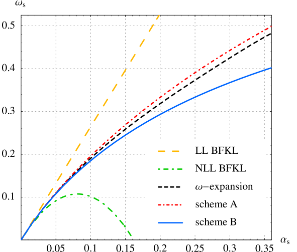
Figure 1: $\omega_{s}$ as a function of $\alpha_{s}$ for different subtraction schemes together with the original result for the $\omega$-expansion. The calculation is done in the fixed coupling case.

In Fig. 1 we compare the results for the exponent $\omega_{s}$ as a function of $\alpha_{s}$ calculated in the case of fixed coupling for schemes $A,B$ and the original $\omega$-expansion method presented in [10, 11]. The critical exponent is obtained by evaluating the effective kernel eigenvalue at the minimum

$$\omega_{s}^{(0)}=\bar{\alpha}_{s}\chi^{(0)}_{{\mathrm{eff}}}(\gamma_{m},\bar{\alpha}_{s})\;.$$ (68)

All resummed results for the intercept are significantly reduced in comparison with the LL result and they all give stable predictions even for large values of $\bar{\alpha}_{s}$. As we see from the plot, the changes of resummation procedure as well as subtraction scheme do not significantly influence the values of $\omega_{s}$. They give at most $20\%$ change at the highest $\alpha_{s}\simeq 0.35$.

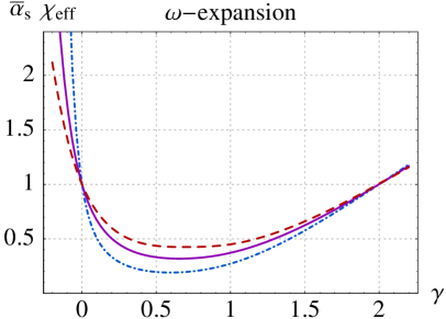
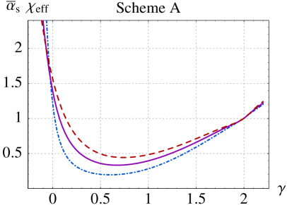
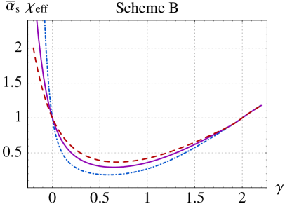
Figure 2: $\bar{\alpha}_{s}\chi_{{\mathrm{eff}}}(\gamma,\bar{\alpha}_{s})$ as a function of $\gamma$ in different schemes for different values of $\alpha_{s}$: $\alpha_{s}=0.1$ (dash-dotted line), $\alpha_{s}=0.2$ (solid line), $\alpha_{s}=0.3$ (dashed line). The calculation is done in the fixed coupling case.

In Fig. 2 we show the effective kernel eigenvalue as a function of $\gamma$. We have considered here the asymmetric $\omega$-shift, which corresponds to the upper energy scale choice $\nu_{0}=k^{2}$. In this case it is easy to show that close to $\gamma=0$ the effective eigenvalues from scheme B and the original $\omega$-expansion [11] satisfy the momentum sum rule. This is illustrated in Fig. 2 by the fact that $\bar{\alpha}_{s}\chi_{{\mathrm{eff}}}(\gamma=0,\bar{\alpha}_{s})=1$ for all values of $\bar{\alpha}_{s}$ in these schemes. This can be seen by expanding around $\gamma=0$, where we have

$$\chi_{\omega}(\gamma,\bar{\alpha}_{s})\propto\frac{1+\omega A_{1}(\omega)}{\gamma}$$ (69)

which for $\gamma=0$ gives $\omega A_{1}(\omega)=-1$, which has the solution $\omega=1$. Note that a second fixed intersection point of curves with different $\alpha_{s}$ occurs at $\gamma=2$. This is expected from energy-momentum conservation in the collinear regime $Q_{0}^{2}\gg Q^{2}$, because of a behavior similar to Eq. (69) around the shifted pole $1+\omega-\gamma=0$. This intersection has no counterpart in the approach of Ref. [12].

We also examine the second derivative $\chi_{{\mathrm{eff}}}^{\prime\prime}(\gamma,\bar{\alpha}_{s})$ which controls the diffusion properties of the small-$x$ equation, Fig. 3. As we see from the plot, the second derivative is more model-dependent than the intercept $\omega_{s}$, though the two models A and B presented in this paper give quite similar answers. The value of the second derivative will influence the diffusion corrections to the hard Pomeron, as we shall see in Sec. 4.4, and also the transition of the solution to the non-perturbative regime.

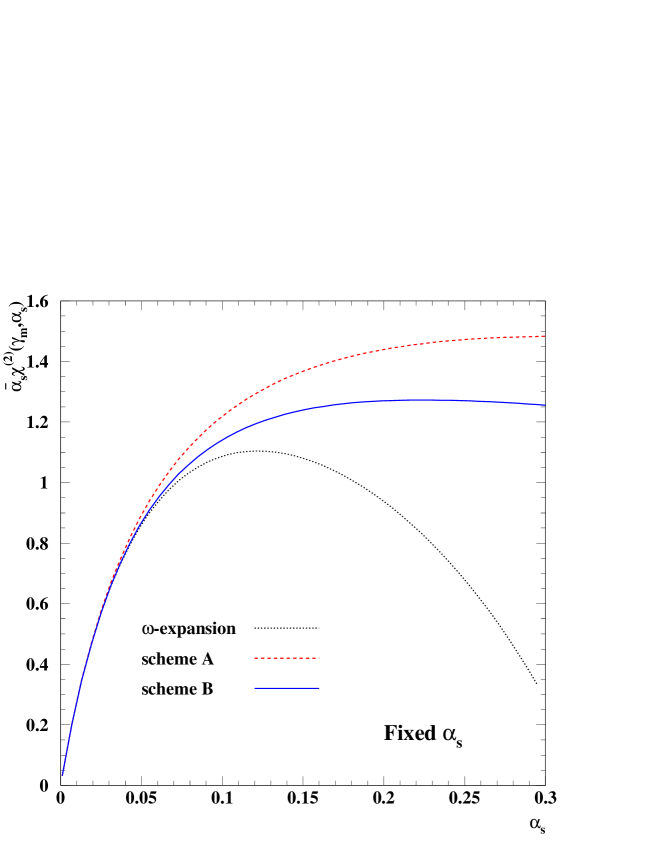
Figure 3: $\chi^{\prime\prime}(\gamma_{m},\bar{\alpha}_{s})$ as a function of $\alpha_{s}$ for two different subtraction models and the $\omega$-expansion scheme.

4.2 Numerical methods for solution

In this section we are going to investigate in detail the shape of the solutions to the integral equation with the resummed kernel given in sections 3.2 and 3.3. To this aim we solve numerically the following integral equation

$$G(Y;k,k_{0})=G^{(0)}(k,k_{0})\Theta(Y)+\int_{0}^{Y}dy\int_{k_{min}}^{k_{max}}dk^{\prime 2}\;{\cal K}(Y-y;k,k^{\prime})G(y;k^{\prime},k_{0})\\$$ (70)

with (so as to have the same normalization as in Eq. (3)),

$$2\pi k_{0}^{2}G^{(0)}(k,k_{0})=\delta(\log\frac{k}{k_{0}})\,.$$

We use the method of iterations and discretized kernel similar to that introduced in [33]. More precisely in our problem (see (47)) we can rewrite the kernel in the following way:

$${\cal K}(Y-y;k,k^{\prime})=\sum_{\alpha}{\cal K}_{\alpha}(Y-y;k,k^{\prime})=\sum_{\alpha}K_{\alpha}(k,k^{\prime})\,P_{\alpha}(Y-y)\,\Theta_{R}\Big{(}Y-y-{\rm max}(\log\frac{k}{k^{\prime}},\log\frac{k^{\prime}}{k})\Big{)}\;,$$ (71)

where the index $\alpha$ enumerates different terms in the equation (47) (that is LL BFKL, LL DGLAP, and the different components of NLL BFKL with subtractions), each of which factorize into transverse and longitudinal parts. The $P_{\alpha}$ are the singular and non-singular pieces of the splitting function as well as the subtraction terms $S_{2}(x)$. The additional $\Theta_{R}$ stands for the kinematical constraint, applied to all terms that in Mellin-space have an $\omega$-shift.

To find the solution numerically one introduces a grid in rapidity $Y$ and logarithm of momentum, $\tau=\log k/k_{0}$, with small spacings, $\Delta Y$ and $\Delta\tau$ respectively. The solution is then calculated at the grid points. Linear interpolation gives the values of the solution in the points between the nodes of the grid

$$G(Y;k,k_{0})=\sum_{i}\sum_{j}\,\phi_{i}(Y)\psi_{j}(k)\,G(Y_{i};k_{j},k_{0})$$ (72)

where $\phi_{i}(Y)$ and $\psi_{j}(k)$ are the appropriate basis functions for linear interpolation. To find the solution for $G$ the equation (70) is solved by a method of evolution in rapidity. In a first step one takes $G(Y_{0}=0;k_{m},k_{0})=G^{(0)}(k_{m},k_{0})$ and estimates $G(Y_{1};k_{m},k_{0})$ at the next point of the grid, $Y_{1}=\Delta Y$, using the integral equation (70). This gives a first approximated value for $G(Y_{1};k_{m},k_{0})$. This function is then again used in equation (70) to calculate the next approximation. Usually a few iterations are sufficient to find an accurate answer (typically $5-8$). After obtaining $G(Y_{1};k_{m},k_{0})$ with the desired accuracy one proceeds to calculate the solution on the next point of the grid $Y_{2}=2\Delta Y$ and so on. The procedure is then repeated for all points of the grid in rapidity $Y_{n}=n\Delta Y$.

The procedure presented above requires numerous evaluations of the right hand side of equation (70). Given the fact that we have two convolutions in $y$ and $k^{\prime}$, with the complicated kernel ${\cal K}$, such a procedure can be quite time consuming.

In order to speed up the calculation one can discretize in $k^{\prime}$ the kernels $K_{\alpha}$ and in $y$ the functions $P_{\alpha}$ using the basis functions in the following form

$$K^{(\alpha)}_{m,i} = \int dk^{\prime 2}\,K_{\alpha}(k_{m},k^{\prime})\,\psi_{i}(k^{\prime})$$

$$P^{(\alpha)}_{n-j} = \int dy\,P_{\alpha}(Y_{n}-y)\,\phi_{j}(y)\;,$$ (73)

where we have used the fact that the functions $P_{\alpha}$ depend only on the difference $Y_{n}-y$ which — together with the linear interpolation — results in a one-dimensional vector $P$ instead of a matrix. One can simplify the treatment of the $\Theta_{R}$ function in (71) by using the same grid spacing in $y$ and in $\log k$, $\Delta y=\Delta\tau$ (or for energy-scale choice $\nu_{0}=k^{2}$, $\Delta y=2\Delta\tau$). After the discretization procedure, the convolution on the right hand side in equation (70) (and using (71)) can be then represented as a multiplication as follows

$$\int dy\int dk^{\prime 2}\;{\cal K}_{\alpha}(Y_{n}-y;k_{m},k^{\prime})\,G(y;k^{\prime},k_{0})=\sum_{i=0}^{i_{max}}\,\sum_{j=0}^{n-|m-i|}\,P^{(\alpha)}_{n-j-|m-i|}\,K^{(\alpha)}_{m,i}\,G(y_{j};k_{i},k_{0})\;,$$ (74)

so that in practice all the integrations present in equations (70) are performed once before the evolution, and then only the multiplications of kernel matrices and gluon Green’s function vectors are done during the iterations.

Of course, in a numerical analysis one is not able to use exact distributions — in particular for the delta function in $k$ as an initial condition, see Eq. (3). In practice what is done is to set to $1/\Delta\tau$ one point on the fine grid i.e. $2\pi k_{0}^{2}G^{(0)}(k_{m},k_{0})=\frac{1}{\Delta\tau}\delta_{m0}$, where $\Delta\tau$ is the grid spacing in $\log k$. The resulting Green’s function will be finite in the $Y=0$ limit but dependent on the size of the grid spacing. We illustrate this effect in the upper set of curves of Fig. 4, where we have solved the equation (70) with the kernel in LL approximation with $3$ different grid spacings $\Delta\tau=0.05,\;0.1,\;0.2$. One might be worried by the apparently substantial dependence on the choice of the grid spacing $\Delta\tau$. However this is just a consequence of the grid-dependent discretization of the initial $\delta$-function and disappears when one convolutes the gluon Green’s function with some smooth impact factor. We will therefore consider from now on a slightly asymmetric choice of scales, $G(Y;t_{0},t_{0}+\epsilon)$ with $\epsilon=0.2$. In the lower set of curves of Fig. 4 one sees that the dependence on the grid spacing in this case is relatively small. For the remaining plots in this paper we have used $\Delta\tau=0.1$ or smaller.

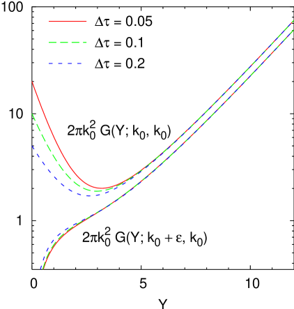
Figure 4: Gluon Green’s function as a function of rapidity $Y$ for three different grid spacings $\Delta\tau=0.05,0.1,0.2$. LL evolution is used with a fixed coupling, $\bar{\alpha}_{s}=0.2$; $\epsilon\simeq 0.2k_{0}$.

4.3 Basic features of the Green’s function

Let us now discuss the properties of the gluon Green’s function obtained with the method discussed above. We shall use a one-loop coupling with $n_{f}=4$, normalized such that $\bar{\alpha}_{s}(9\,\,\mathrm{GeV}^{2})=0.244$. The coupling is cut off at scale ${\bar{k}}=0.74\,\,\mathrm{GeV}$ — a detailed analysis of the sensitivity to this regularization is postponed to section 4.5. In the kernel, for the time being we consider $n_{f}=0$, since our single-channel RGI approach does not properly account for the quark sector (however we will see below that simply varying $n_{f}$ in the kernel has only a small effect).

Results will be given given for: LL evolution (with $\bar{\alpha}_{s}(q^{2})$); our two resummation schemes, A and B; and two variants of ‘pure’ NLL evolution: one, labeled ‘NLL $\alpha_{s}(q^{2})$’ where the kernel is $\bar{\alpha}_{s}(q^{2})K_{0}+\bar{\alpha}_{s}^{2}(k_{>}^{2})K_{1}^{b=0}$, with $K_{1}^{b=0}$ corresponding to eq. (19) without the first term in square brackets; and another, labeled ‘NLL $\alpha_{s}(k^{2})$’, where the kernel is $\bar{\alpha}_{s}(k^{2})K_{0}+\bar{\alpha}_{s}^{2}(k^{2})K_{1}$, and $K_{1}$ corresponds to eq. (19) in full.

Fig. 5 shows Green’s functions $G(Y;k_{0}+\epsilon,k_{0})$ as a function of rapidity $Y$, and fig. 6 shows $kk_{0}G(Y;k,k_{0})$ as a function of $k$ for $Y=10$. To aid legibility, each figure has been separated into two plots, the left-hand one (a) showing LL and schemes A and B, while the right-hand one (b) shows the two pure NLL curves and scheme B. We choose a moderately high value for the initial transverse scale, $k_{0}=20\,\,\mathrm{GeV}$, $\bar{\alpha}_{s}(k_{0})\simeq 0.15$, so as to be able to focus on the perturbative aspects of the problem (non-perturbative effects are formally suppressed by powers of $\Lambda^{2}/k_{0}^{2}$). Such a scale has been used for BFKL dijet studies at the Tevatron [46].

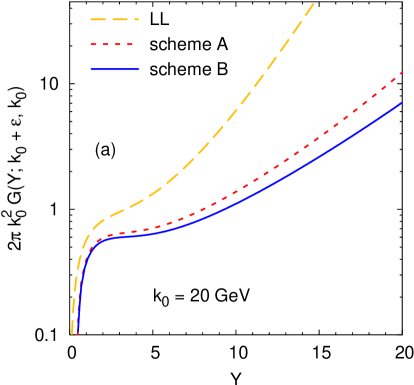
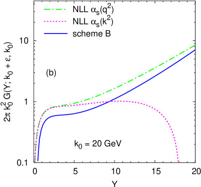
Figure 5: Gluon Green’s function $G(Y;k_{0}+\epsilon,k_{0})$ as a function of rapidity $Y$: (a) for LL and the two RGI schemes A and B; (b) for scheme B and two variants of pure NLL evolution. The parameters are $k_{0}=20\,\,\mathrm{GeV}$ and $\epsilon\simeq 0.2k_{0}$.

A number of features of fig. 5a are worth commenting. Most noticeable is the significant reduction in the high-energy growth of the Green’s function when going from LL evolution to our resummed schemes A and B. This is as expected from the discussion of high-energy exponents, fig. 1. Also important is the fact that for the RGI schemes the high-energy growth does not start until a rapidity of about $4$. Both of these observations are relevant to the problem of trying to reconcile theoretical predictions with the lack of experimental evidence for a strong high-energy growth of cross sections at today’s energies. The small difference between the two RGI resummation schemes, A and B, is in accord with their slightly different $\omega_{s}$ values (cf. fig. 1).

As regards the transverse momentum dependence of the Green’s function, fig. 6a there are a number of further differences between the LL and RGI results. The higher overall normalization for LL evolution is just a consequence of a larger $\omega_{s}$ value. But one also sees that the large-$k$ tails in $k$ for the resummed models are substantially steeper than in the LL case. This can be understood by comparing the diffusion coefficients in these models: the RGI models are characterized by a smaller $\chi^{\prime\prime}_{{\mathrm{eff}}}$ and, as a consequence, they have less diffusion than in the LL case. As was the case for the $Y$ dependence, the two RGI schemes give very similar results, here differing essentially only in the normalization.

Some comments are due concerning the structure at low $k$: there, there is a component of the evolution that is sensitive to the larger coupling, $\alpha_{s}(1\,\,\mathrm{GeV}^{2})\simeq 0.4$. For the LL case the resulting stronger evolution (than at $k_{0}^{2}$) over-compensates the suppression due to the large ratio of scales $k_{0}/k$, leading to the absence of a decreasing low-$k$ tail. For the RGI schemes the difference between $\omega_{s}$ values at $1\,\,\mathrm{GeV}$ and $k_{0}$ is not sufficient to bring about this overcompensation for $Y=10$, so there still is a decreasing tail for small $k$. However the results are sensitive to the fact that at large $\alpha_{s}$ the difference between $\omega_{s}$ values for the two schemes becomes non-negligible. This is what causes the low-$k$ Green’s function to be almost three times larger for scheme A than scheme B. It should of course be kept in mind that all the properties at low $k$ are strongly dependent on the particular choice of infrared regularization of the coupling.

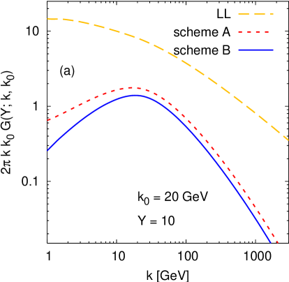
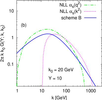
Figure 6: Gluon Green’s function $2\pi kk_{0}G(Y;k,k_{0})$ at rapidity $Y=10$ as a function of the transverse scale $k$. The sets of kernels used in plots (a) and (b) are the same as in figure 5.

Let us now examine the right-hand plots of figures 5 and 6, which show results with pure NLL evolution. We recall that the original motivation for introducing RGI resummation schemes was the large size of the NLL corrections, and in particular the fact that for moderate values of the coupling the NLL terms change the sign of $\chi(\gamma)$ and its second derivative around $\gamma=1/2$, with the situation being even worse in the collinear region. Nevertheless, as was pointed out by Ross [7], because of the change of sign of $\chi^{\prime\prime}(\frac{1}{2})$, the usual saddle point at $\gamma=\frac{1}{2}$ is replaced by two saddle points off the real axis, at $\gamma=1/2+i\nu_{0}$ and $1/2-i\nu_{0}^{*}$, and it is the value of $\chi$ at these new saddle points that determines the high-energy behavior of the (fixed-coupling) NLL Green’s function:

$$\pi kk_{0}G(Y;k,k_{0})=\int\frac{d\gamma}{2\pi i}e^{\bar{\alpha}_{s}Y\chi(\gamma)}\left(\frac{k^{2}}{k_{0}^{2}}\right)^{\gamma-\frac{1}{2}}\sim e^{\bar{\alpha}_{s}Y\chi(\frac{1}{2}+i\nu_{0})}\left(\frac{k^{2}}{k_{0}^{2}}\right)^{i\nu_{0}}+e^{\bar{\alpha}_{s}Y\chi(\frac{1}{2}-i\nu_{0}^{*})}\left(\frac{k^{2}}{k_{0}^{2}}\right)^{-i\nu_{0}^{*}}\,.$$ (75)

Since $\chi(\gamma)=\chi^{*}(\gamma^{*})$ this gives

$$\pi kk_{0}G(Y;k,k_{0})\sim e^{\bar{\alpha}_{s}Y\Re[\chi(\frac{1}{2}+i\nu_{0})]-\Im[\nu_{0}]\log\frac{k^{2}}{k_{0}^{2}}}\cos\left(\Re[\nu_{0}]\log\frac{k^{2}}{k_{0}^{2}}+\bar{\alpha}_{s}Y\,\Im[\chi(\frac{1}{2}+i\nu_{0})]\right)\,.$$ (76)

When $\chi_{1}(\gamma)$ is symmetric in $\gamma\leftrightarrow 1-\gamma$, as is the case if we use $\alpha_{s}(q^{2})$ in the LL term (or as can be achieved with the modified Mellin transform suggested in [4] and used in [7]), then $\bar{\alpha}_{s}\chi(\frac{1}{2}+\nu_{0})$ is real, having a value of about $0.2$. One therefore expects to find a high-energy growth of the Green’s function that numerically is not so different from that with out RGI resummed schemes. This is precisely what is observed in fig. 5b for the ‘NLL $\alpha_{s}(q^{2})$’ result.

On the other hand if $\chi_{1}(\gamma)$ is not symmetric in $\gamma\leftrightarrow 1-\gamma$ then $\chi$ will be complex at the saddle points. This is the case for the ‘NLL $\alpha_{s}(k^{2})$’ kernel and the change in sign of the Green’s function around $Y=18$ can be understood as a direct consequence of a zero of eq. (76) when $\bar{\alpha}_{s}Y\,\Im[\chi(\frac{1}{2}+i\nu_{0})]=\pi/2$.

The oscillatory behavior of eq. (76) also becomes an issue when $k\neq k_{0}$, as is visible in fig. 6b. For NLL evolution with $\alpha_{s}(q^{2})$ the change of sign intervenes only for ratios of $k/k_{0}$ that are fairly small or large from a phenomenological point of view (at least for Mueller-Navelet or $\gamma^{*}\gamma^{*}$ type processes). For evolution with $\alpha_{s}(k^{2})$ the situation is more dramatic because of the sum of terms in the argument of the cosine of eq. (76).

So our overall conclusions regarding NLL evolution is that, while in certain instances it may give results that are not too different from those with RGI methods, in general it offers only limited predictive power, because of the strong sensitivity to the details of the formulation. Though here we have just discussed renormalisation scale sensitivity, we note that changing the energy scale $\nu_{0}$ from say $kk_{0}$ to $k^{2}$ also leads to a Green’s function that oscillates as a function of $Y$, since once again the characteristic function is asymmetric.

A final point relating to figures 5 and 6 concerns the overall normalization of the results. One sees that at low $Y$ the LL and NLL results all have similar normalizations, while the RGI results are slightly lower. This is because the $\omega$-dependence is associated with an implicit NLO impact factor. This of course has to be taken into account should one wish to use the RGI Green’s function in conjunction with any NLO impact factor calculation, as is discussed in detail in section 6. To close this section we present brief results on $n_{f}$ and renormalisation scale dependence for the RGI schemes.

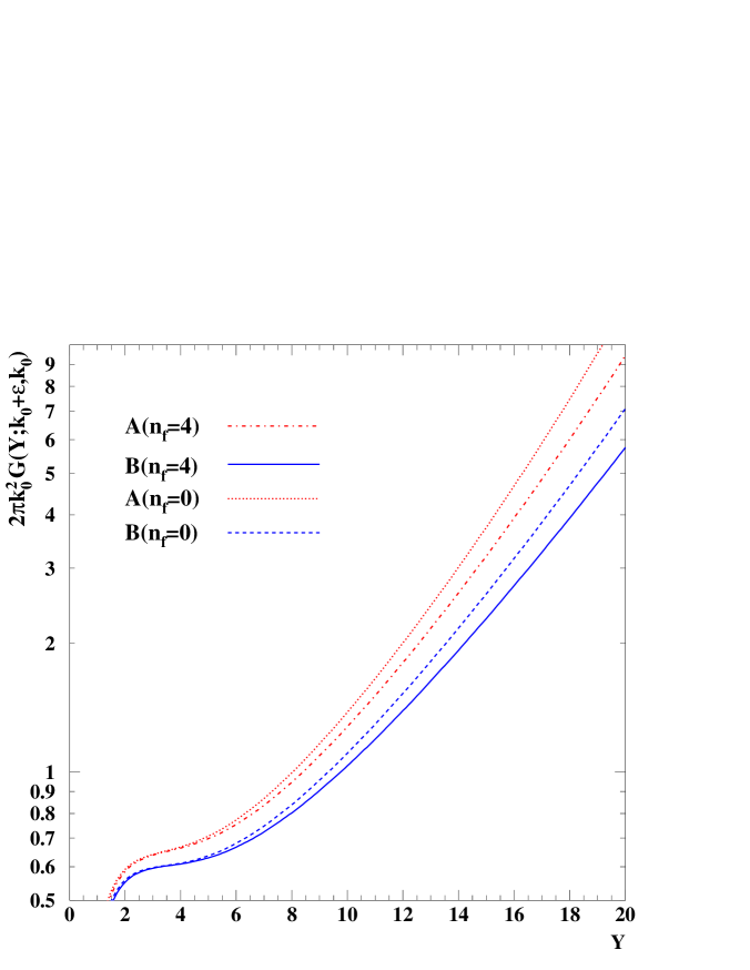
Figure 7: Gluon Green’s function $G(Y;k_{0},k_{0}+\epsilon)$ as a function of rapidity $Y$ for two different resummation schemes $A,B$ in the $n_{f}=0,4$ cases. Parameter $\epsilon\simeq 0.2k_{0}$

Our RGI approach has been constructed for a purely gluonic channel and only scheme B satisfies the momentum sum rule in this case. For phenomenological purposes one would wish to include quarks and in Fig. 7 we present the two schemes in the cases when $n_{f}=0$ and $n_{f}=4$ in the NLL kernel. As is clear from the plot, having $n_{f}\neq 0$ does not change the result in a significant way. We note that the full inclusion of quarks in a RG-consistent manner is a non-trivial operation in this framework especially if one is to construct resummed quark anomalous dimensions that satisfy the momentum sum rules.

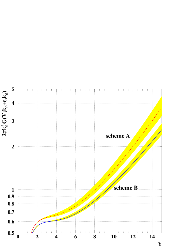
Figure 8: Gluon Green’s function $G(Y;k_{0},k_{0}+\epsilon)$ as a function of rapidity $Y$ for two different resummation models $A,B$. The bands represent the uncertainty due to a variation of the renormalisation scale in the range $1/2<x_{\mu}^{2}<2$. Parameter $\epsilon\simeq 0.2k_{0}$

Finally, we show the dependence of the gluon Green’s function on the renormalisation scale choice eq. (42). We have varied the scale $x_{\mu}$ in the range $1/2<x^{2}_{\mu}<2$. The results of the calculation are presented in Fig. 8 where the yellow bands correspond to the renormalisation scale variation for two resummation schemes.

4.4 $\boldsymbol{b}$-expansion of intercept and of diffusion coefficient

In order to properly evaluate the hard Pomeron intercept $\omega_{s}$ in the case with running coupling it is necessary to control the corrections with respect to the frozen coupling limit. To this end we shall apply the $b$-expansion method presented in [23].

According to this method, we use the formal limit $b\to 0$ (with $\alpha_{s}(t_{0})$ kept fixed) in order to suppress the non-perturbative Pomeron. The left-over perturbative Green’s function can then be expanded in $b$ in the form

$$G(Y;t_{0},t_{0})=G^{(0)}(Y;t_{0},t_{0})\exp\left[b\omega_{s}^{(1)}Y+{\cal O}(b^{2}\alpha_{s}^{5}Y^{3})\right]\left(1+{\cal O}(b^{2}\alpha_{s}^{4}Y^{2})\right)\;,$$ (77)

which shows a shift of $\omega_{s}$ of order $b\alpha_{s}^{2}$, as well as diffusion corrections of order $(b\alpha_{s})^{2}(\omega_{s}Y)^{2}$ and $(b\alpha_{s})^{2}(\omega_{s}Y)^{3}$. The purpose of this subsection is to compute $\omega_{s}^{(1)}$ [defined by Eq. (77)] and the $Y^{3}$ terms both analytically and numerically. Further corrections to $\omega_{s}$ of order $b^{2}\alpha_{s}^{3}$ appear as subleading contributions in this expansion and are probably not really meaningful, given the complex $Y$-dependence of the exponent involving the parameter $b\alpha_{s}^{2}Y$ [23].

We start by expanding the $\alpha_{s}$-dependence of the kernel around the frozen-coupling limit up to ${\cal O}(b^{2})$ by setting, for instance at scale $q^{2}$,

$$\alpha_{s}(q^{2})-\alpha_{s}(k_{0}^{2})=-b\alpha_{0}^{2}\left(\log\frac{q^{2}}{k^{2}}+(t-t_{0})\right)+b^{2}\alpha_{0}^{3}\left(\log^{2}\frac{q^{2}}{k^{2}}+2(t-t_{0})\log\frac{q^{2}}{k^{2}}+(t-t_{0})^{2}\right)\;,$$ (78)

where $\alpha_{0}\equiv\bar{\alpha}_{s}(k_{0}^{2})$ throughout this section. We then define the kernel with frozen-coupling ${\cal K}_{\omega}^{(0)}\equiv\left.{\cal K}_{\omega}\right|_{\bar{\alpha}_{s}\to\alpha_{0}}$ and the correction kernel $\Delta$ as

$$\Delta(t,t^{\prime}) \equiv{\cal K}_{\omega}-{\cal K}_{\omega}^{(0)}={\cal K}_{\omega}-\alpha_{0}\left(K_{0}^{\omega}+\omega K_{\mathrm{c}}^{\omega}\right)-\alpha_{0}^{2}\tilde{K}_{1}^{\omega}$$ (79)

$$=\Delta_{0}(t-t^{\prime})+(t_{0}-t)\Delta_{1}(t-t^{\prime})+(t_{0}-t)^{2}\Delta_{2}(t-t^{\prime})\;,$$ (80)

where the $\Delta_{i}$’s are scale-invariant, and are obtained from the definition (47) by picking up the relevant terms in the running coupling expansions of type (78). We obtain:

$$\Delta_{0} =-b\alpha_{0}^{2}\left[\log\frac{q^{2}}{k^{2}}K_{0}^{\omega}+\log\frac{k_{>}^{2}}{k^{2}}(\omega K_{\mathrm{c}}^{\omega}+2\alpha_{0}\tilde{K}_{1}^{\omega})\right]+{\cal O}(b^{2}\alpha_{0}^{3})$$ (81a)

$$\Delta_{1} =b\alpha_{0}^{2}\left[K_{0}^{\omega}+\omega K_{\mathrm{c}}^{\omega}+2\alpha_{0}\tilde{K}_{1}^{\omega}\right]+{\cal O}(b^{2}\alpha_{0}^{3})$$

$$=b\alpha_{0}^{2}\frac{\partial}{\partial\alpha_{0}}K_{\omega}^{(0)}(\alpha_{0};k^{2},k_{0}^{2})+{\cal O}(b^{2}\alpha_{0}^{3})$$ (81b)

$$\Delta_{2} =b^{2}\alpha_{0}^{3}\left[(K_{0}^{\omega}+\omega K_{\mathrm{c}}^{\omega})+3\alpha_{0}\tilde{K}_{1}^{\omega}\ \right]\;.$$ (81c)

Now we evaluate the Green’s function $G_{\omega}(t,t_{0})$ in $\omega$-space up to second order in $b$, with the purpose of deriving the leading diffusion terms $\sim b^{2}Y^{3}$ and the intercept shift at ${\cal O}(b)$; to this purpose, expansion (81) is sufficient. We have

$$G=G^{(0)}+G^{(1)}+G^{(2)}+\cdots$$ (82)

with

$$G^{(0)} =\big{[}\omega-K_{\omega}^{(0)}\big{]}^{-1}$$ (83a)

$$G^{(1)} =G^{(0)}\Delta\;G^{(0)}=\int\frac{d\gamma}{2\pi i}\;e^{(\gamma-{\textstyle\frac{1}{2}})(t-t_{0})}G^{(0)}(\gamma)\left[\Delta_{0}G^{(0)}+\Big{(}\Delta_{1}G^{(0)}\Big{)}^{\prime}+\Big{(}\Delta_{2}G^{(0)}\Big{)}^{\prime\prime}\right](\gamma)$$ (83b)

$$G^{(2)} =G^{(0)}\Delta\;G^{(1)}=\int\frac{d\gamma}{2\pi i}\;e^{(\gamma-{\textstyle\frac{1}{2}})(t-t_{0})}G^{(0)}(\gamma)\left[\Delta_{0}G^{(1)}+\Big{(}\Delta_{1}G^{(1)}\Big{)}^{\prime}+\Big{(}\Delta_{2}G^{(1)}\Big{)}^{\prime\prime}\right](\gamma)$$ (83c)

where, inside the integrals, we have used the same notation for the kernels and their $\gamma$-space eigenvalues. We restrict our attention to $t=t_{0}$ and perform partial integrations to obtain

$$G^{(1)}_{\omega}(t_{0},t_{0}) =\int\frac{d\gamma}{2\pi i}\;\left[\Big{(}\Delta_{0}+\frac{1}{2}\Delta_{1}^{\prime}\Big{)}G^{(0)2}+\Delta_{2}\left(\frac{1}{2}\Big{(}G^{(0)2}\Big{)}^{\prime\prime}-\Big{(}G^{(0)}{}^{\prime}\Big{)}^{2}\right)\right]$$

$$=\int\frac{d\gamma}{2\pi i}\;\left[\frac{\Delta_{0}+\frac{1}{2}\Delta_{1}^{\prime}+\frac{1}{3}\Delta_{2}^{\prime\prime}}{\big{[}\omega-\chi_{\omega}^{(0)}\big{]}^{2}}+\frac{1}{3}\,\frac{\Delta_{2}\chi_{\omega}^{(0)}{}^{\prime\prime}}{\big{[}\omega-\chi_{\omega}^{(0)}\big{]}^{3}}\right]\;,$$ (84)

where the $\gamma$-variable dependence is understood in the $\Delta$’s, $G$’s and $\chi$’s. Up to this order, the maximal energy dependence comes from the cubic pole, which yields a $\sim b^{2}\alpha_{0}^{3}Y^{2}$ dependence. The double pole yields instead terms $\sim b\alpha_{0}^{2}Y$ which provide the ${\cal O}(b)$ correction to $\omega_{s}$. By noting that

$$G^{(0)}(Y;t_{0},t_{0}) =\int\frac{d\gamma}{2\pi i}\frac{d\omega}{2\pi i}\;\frac{e^{\omega Y}}{\omega-\chi_{\omega}^{(0)}(\gamma)}\simeq\frac{Je^{\omega_{s}^{(0)}Y}}{\sqrt{4\pi D\omega_{s}^{(0)}Y}}$$ (85)

$$J =\left[1-\partial_{\omega}\chi_{\omega}^{(0)}({\textstyle\frac{1}{2}})\right]^{-1}_{\omega=\omega_{s}^{(0)}}\;,$$ (86)

and that a squared Jacobian factor $J^{2}$ occurs in $G^{(1)}$, we obtain the ${\cal O}(b)$ correction

$$b\omega_{s}^{(1)}=\left[\Delta_{0}({\textstyle\frac{1}{2}})+\frac{1}{2}\Delta_{1}^{\prime}({\textstyle\frac{1}{2}})\right]J\;,$$ (87)

where actually $\Delta_{1}^{\prime}({\textstyle\frac{1}{2}})=0$, because $\Delta_{1}(\gamma)$ is symmetric for $\gamma\leftrightarrow 1-\gamma$.

The eigenvalue function $\Delta_{0}(\gamma)$ is found from the definition in Eq. (81a) by noting that the generalized regularized kernel

$$\frac{1}{\pi\boldsymbol{q}^{2}}\left(\frac{\boldsymbol{q}^{2}}{{\boldsymbol{k}}^{2}}\right)^{\lambda}\left(\frac{k_{<}}{k_{>}}\right)^{\omega}-\frac{1}{\lambda}\delta^{2}(\boldsymbol{q})\;,$$ (88)

has characteristic function $\chi_{L}^{[\lambda]}(\gamma+{\textstyle\frac{\omega}{2}})+\chi_{R}^{[\lambda]}(1-\gamma+{\textstyle\frac{\omega}{2}})$, where

$$\chi^{[\lambda]}(\gamma)=\frac{1}{\lambda}\left[\exp\left(\lambda\chi_{0}(\gamma)+\frac{1}{2}\lambda^{2}\chi_{0}^{\prime}(\gamma)+{\cal O}(\lambda^{3})\right)-1\right]\;,$$ (89)

and the subscript $L$ ($R$) refers to the projection with left-hand (right-hand) poles. By proper expansion in $\lambda$ we obtain (See App. A)

$$\Delta_{0}(\gamma)+\frac{1}{2}\Delta_{1}^{\prime}(\gamma)=-\frac{b\alpha_{0}^{2}}{2}\left\{[\chi_{0}^{2}]_{L}(\gamma+{\textstyle\frac{\omega}{2}})-\omega\chi_{{\mathrm{c}}L}^{\prime}(\gamma+{\textstyle\frac{\omega}{2}})-2\alpha_{0}\tilde{\chi}_{1L}^{\omega}{}^{\prime}(\gamma)+[\gamma\leftrightarrow 1-\gamma]\right\}\;,$$ (90)

and finally

$$\omega_{s}^{(1)}=-\alpha_{0}^{2}\Big{[}[\chi_{0}^{2}]_{L}({\textstyle\frac{1+\omega}{2}})-\omega\chi_{{\mathrm{c}}L}^{\prime}({\textstyle\frac{1+\omega}{2}})-2\alpha_{0}\tilde{\chi}_{1L}^{\omega}{}^{\prime}({\textstyle\frac{1}{2}})\Big{]}J+\cdots\;.$$ (91)

We note that the expressions of the left projections are (See App. A)

$$\chi_{0L}(\gamma) =\psi(1)-\psi(\gamma)\;,$$ (92)

$$[\chi_{0}^{2}]_{L}(\gamma) =2[\chi_{0L}(\gamma)]^{2}-\psi^{\prime}(\gamma)+\frac{\pi^{2}}{2}$$ (93)

$$\chi_{{\mathrm{c}}L}(\gamma) =\frac{A_{1}(\omega)}{\gamma}\;,$$ (94)

and $\tilde{\chi}_{1L}(\gamma)$, depending on the resummation scheme, is quoted in App. A.

While the $\sim b^{2}Y^{2}$ terms exponentiate $\Delta\omega_{s}$ and provide a further normalization correction [23], the $\sim b^{2}Y^{3}$ terms provide the leading diffusion corrections and occur in $G^{(2)}$. Considering Eq. (83c) for $t=t_{0}$ and performing partial integrations, we obtain at ${\cal O}(b^{2})$

$$G_{\omega}^{(2)}(t_{0},t_{0}) \simeq\int\frac{d\gamma}{2\pi i}\;\left[\Delta_{0}G^{(0)}-\Delta_{1}G^{(0)}{}^{\prime}\right]G^{(0)}\left[\Delta_{0}G^{(0)}+\Big{(}\Delta_{1}G^{(0)}\Big{)}^{\prime}\right]$$

$$=\int\frac{d\gamma}{2\pi i}\;\left[\Big{(}\Delta_{0}G^{(0)}\Big{)}^{2}-\Delta_{1}G^{(0)}{}^{\prime}\Big{(}\Delta_{1}G^{(0)}\Big{)}^{\prime}\right]G^{(0)}\;.$$ (95)

This result contains up to a fifth order pole, which can be reduced to a quartic one by partial integration, to yield

$$G^{(2)}(Y;t_{0},t_{0}) \simeq\int\frac{d\gamma}{2\pi i}\frac{d\omega}{2\pi i}\;e^{\omega Y}\frac{1}{4}\,\frac{\Delta_{1}^{2}\chi_{\omega}^{(0)}{}^{\prime\prime}}{\big{[}\omega-\chi_{\omega}^{(0)}\big{]}^{4}}$$

$$\simeq\int\frac{d\gamma}{2\pi i}\;e^{\bar{\alpha}_{s}\chi_{\mathrm{eff}}(\gamma)Y}\frac{Y^{3}}{24}\,\frac{\chi_{\omega}^{(0)}{}^{\prime\prime}(\gamma)\left[\partial_{\log k_{0}^{2}}\chi_{\omega}^{(0)}(\gamma,\alpha_{s}(k_{0}^{2}))\right]^{2}}{\big{[}1-\partial_{\omega}\chi_{\omega}^{(0)}(\gamma)\big{]}^{4}}$$

$$\simeq G^{(0)}(Y;t_{0},t_{0})\frac{Y^{3}}{24}\left[\partial_{t_{0}}\omega_{s}^{(0)}(t_{0})\right]^{2}\bar{\alpha}_{s}\chi_{\mathrm{eff}}^{\prime\prime}({\textstyle\frac{1}{2}})\;.$$ (96)

The last factor provides the leading diffusion exponent we were looking for. Note that the Jacobian factor $J^{3}$ has been reabsorbed in the $t_{0}$-derivative of $\omega_{s}$ and in the curvature of the effective characteristic function: $\chi_{\mathrm{eff}}^{\prime\prime}({\textstyle\frac{1}{2}})=J\left.\chi_{\omega}^{\prime\prime}({\textstyle\frac{1}{2}})\right|_{\omega=\alpha_{s}\chi_{\mathrm{eff}}}$. This particular form for the generalization of the LO $Y^{3}$ diffusion term is quite natural when one considers the physical mechanism at play: diffusion causes a symmetric spread over a logarithmic range of transverse scales of order $\sqrt{\bar{\alpha}_{s}\chi_{\mathrm{eff}}^{\prime\prime}Y}$. The exponent of the evolution at a scale $t^{\prime}$ is given by $\omega_{s}^{(0)}(t_{0})+(t^{\prime}-t_{0})\partial_{t_{0}}\omega_{s}^{(0)}(t_{0})$. In a first-order expansion of the evolution there is a cancellation between components above and below $t_{0}$. But in a second order expansion of the evolution, there are corrections from above and below $t_{0}$ that enter with the same sign, $\sim[\pm\sqrt{\bar{\alpha}_{s}\chi_{\mathrm{eff}}^{\prime\prime}Y}\partial_{t_{0}}\omega_{s}^{(0)}(t_{0})Y]^{2}$. This is precisely the form of (96).

The analytical treatment given above has its counterpart in the numerical extraction of the running-coupling diffusion coefficients presented in [23]. We illustrate here that the method can also be applied to a more general case with an $\omega$-dependent resummed NLL BFKL kernel.

Formally we write the logarithm of the Green’s function as a power series in $b$:

$$\log G(Y;t;t_{0})=\sum_{i=0}b^{i}\,[\log G(Y;t;t_{0})]_{i}\,,$$ (97)

where the expansion is defined such that $\alpha_{s}(t_{0})$ (or optionally some other scale) is kept independent of $b$. We can then write the effective exponent

$$\omega_{{\mathrm{eff}}}(Y;t_{0})=\frac{d}{dY}\log G(Y;t_{0};t_{0})\,,$$ (98)

also as a series in $b$:

$$\omega_{{\mathrm{eff}}}(Y;t_{0})=\sum_{i=0}b^{i}\omega_{{\mathrm{eff}},i}=\sum_{i=0}b^{i}\frac{d}{dY}[\log G(Y;t_{0};t_{0})]_{i}\,.$$ (99)

In practice the power series is determined numerically by carrying out the evolution with a generalized $b$-dependent coupling $\bar{\alpha}_{s}^{[b]}(k^{2})$,

$$\bar{\alpha}_{s}^{[b]}(k^{2})=\frac{\bar{\alpha}_{s}(k_{0}^{2})}{1+(t-t_{0})b\bar{\alpha}_{s}(k_{0}^{2})}.$$ (100)

using several values of $b=i\delta b$ (typically $\delta b=0.01$ and $i$ ranges from $-3$ to $3$). In the formal limit of small $\delta b$, the knowledge of $\log G(Y;t_{0};t_{0})$ for $n$ values of $b$ allows one to determine the power series up to order $b^{n-1}$.

In Fig. 9 we test the analytical prediction for the leading diffusion term $\sim Y^{3}$ as given by Eq. (96). We show on this plot the term $\omega_{{\mathrm{eff}},2}$ from expansion (99) with the subtracted $\partial_{Y}Y^{3}$ term calculated for schemes A and B with scale $\bar{\alpha}_{s}(q^{2})$ as a function of rapidity $Y$. We clearly see that after the subtraction there is only a linear dependence left, which signals presence of the subleading $\partial_{Y}Y^{2}$ terms

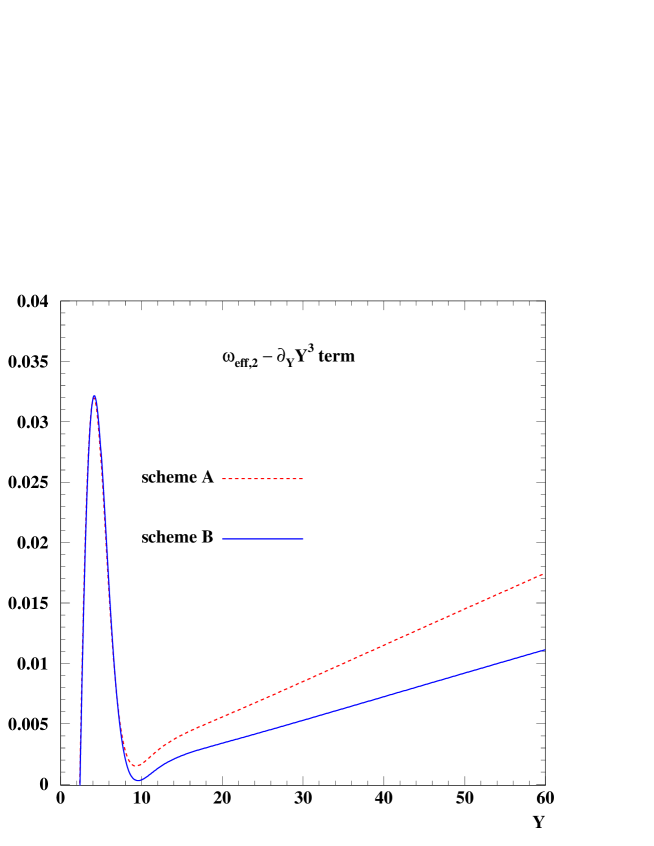
Figure 9: The difference between the $\omega_{{\mathrm{eff}},2}$ coefficient as from (99) and the leading diffusion term calculated from equation (96) for resummed kernel in schemes A (dashed line) and B(solid line). The $b$-expansion has been performed around the fixed coupling value $\bar{\alpha}_{s}(k_{0}^{2})=0.1$.

The numerical value of the diffusion terms is much lower in the resummed models than in the LL BFKL equation. For example the coefficient of the leading $\sim Y^{3}$ term, see (96) in the LL BFKL case is about $8$ times larger than the one in the resummed models. As a consequence the regime in which the solution is perturbative is much broader in the case of the NLL BFKL. One can see this by studying the contour plots in Fig. (14), as will be discussed in more detail in the next section. In particular one finds, Fig. (14a), that the region where the LL solution is insensitive to non-perturbative results is much smaller than in Figs. (14b,c,d) with the resummed evolution. This result is quite encouraging as far as the phenomenological predictions for high energy processes with two hard scales are concerned.

In principle, one could extend our procedure to extract the $Y^{2}$ terms too, as has been done in ref. [23] for the case of the LL BFKL with running coupling. However, the analytical calculation here would be quite involved, since these terms originate from a number of different sources, i.e. they come both from (84) and (95), and moreover they mix with the terms coming from the normalization. In practice these $Y^{2}$ terms are expected to be rather small and not as relevant for phenomenology as the leading $Y^{3}$ terms.

We restrict therefore ourselves to showing only the ${\cal O}(b)$ shift to $\omega_{s}$ given by the analytical expression Eq. (91) and compared with the numerical calculation, see Fig. 10. There is clearly a perfect agreement between the two methods, exhibiting the leading $\alpha_{0}^{2}$ behavior of $\omega_{s}^{(1)}$.

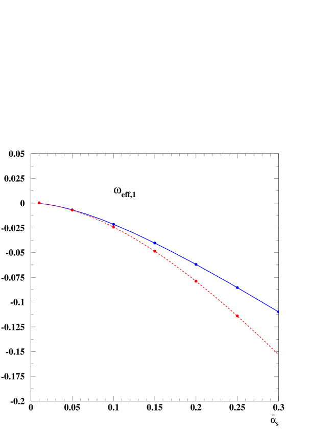
Figure 10: $\omega_{{\rm eff},1}$ from Eq. (99) as a function of the coupling $\bar{\alpha}_{s}$ calculated in schemes A(dashed) and B(solid). Lines represent analytical evaluation based on Eq. (91), the points correspond to the numerical extraction.

Finally, we show in Fig. 11 our numerical evaluation of the sum of the first two terms of $\omega_{\rm eff}$, Eq.(99), that is $\omega^{(0)}+b\omega^{(1)}$, as a function of the coupling constant $\bar{\alpha}_{s}$. The correction due to the running of the coupling reduces somewhat the value of the intercept, as compared with the fixed coupling case ($b=0$), which is shown in Fig. 1.

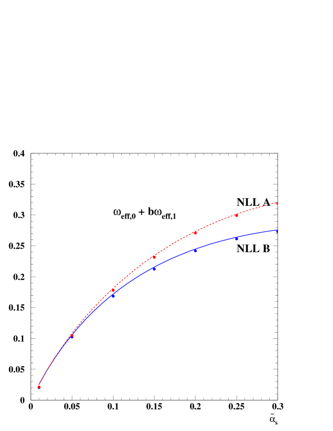
Figure 11: Sum of the first two terms from Eq. (99) as a function of the coupling $\bar{\alpha}_{s}$ calculated in schemes A(dashed) and B(solid).

The plot in Fig. 11 summarizes our present understanding of $\omega_{s}$, because the higher order terms $\sim b^{2}\alpha_{s}^{3},\cdots$ are beyond our present level of accuracy, and are perhaps not really meaningful, given the complex $Y$-dependence of (77).

Note that we do not compare directly with our earlier results for $\omega_{s}$ [11], because they are based on a different definition (the saddle-point of an effective characteristic function), which is less directly related to the Green’s function. Nevertheless, the present results are consistent with previous ones to within NNLL uncertainties.

4.5 NP uncertainties on Green’s function

It is well appreciated nowadays that, even with two hard scales, the ultra-high energy behavior of the BFKL Green’s function is entirely determined by non-perturbative physics. It is only in an intermediate high-energy regime that one is able to make reliable perturbative predictions [16, 17, 18, 22].

Traditionally one estimates non-perturbative uncertainties on BFKL evolution by examining the sensitivity to variations of the infrared regularization of the coupling. More recently we showed that a purely perturbative answer can be defined in the context of the $b$-expansion [23], with the highest perturbatively accessible rapidity being determined by the breakdown of convergence of this expansion. In this section we shall examine both approaches.

Let us consider a variety of infrared (IR) regularizations of the coupling. Mostly we shall use cutoff regularizations,

$$\bar{\alpha}_{s}(q^{2})\equiv\bar{\alpha}_{s}^{\mathrm{PT}}(q^{2})\Theta(q-{\bar{k}})\,,$$ (101)

with three different values of ${\bar{k}}$. It will also be instructive to examine a ‘freezing’ regularization,

$$\bar{\alpha}_{s}(q^{2})\equiv\bar{\alpha}_{s}^{\mathrm{PT}}(\max(q^{2},{\bar{k}}^{2}))\,.$$ (102)

We believe this freezing regularization to be somewhat less physical, since it allows diffusion to arbitrarily low scales in the infrared, in contradiction with confinement. However for the purposes of our general discussion it will be helpful to have it too at our disposal.

In all cases $\bar{\alpha}_{s}^{\mathrm{PT}}$ is the perturbative one-loop coupling with $n_{f}=4$, chosen such that $\bar{\alpha}_{s}(9\,\,\mathrm{GeV}^{2})=0.244$, and no cutoff is placed on exchanged gluon virtualities. The complete set of IR regularizations is summarized in table 1, together with the resulting Pomeron properties, both for LL and resummation scheme B (NLL_B) evolution.

${\bar{k}}$ (GeV)	$\bar{\alpha}_{s}({\bar{k}}^{2})$	asymptotic growth	$\omega_{\mathbb{P}}$ (LL)	$\omega_{\mathbb{P}}$ (NLLB)
1.00 (cutoff)	0.39	$\exp(\omega_{\mathbb{P}}Y)$	0.44	0.32
0.74 (cutoff)	0.46	$\exp(\omega_{\mathbb{P}}Y)$	0.49	0.35
0.50 (cutoff)	0.62	$\exp(\omega_{\mathbb{P}}Y)$	0.58	0.41
0.74 (frozen)	0.46	$Y^{-3/2}\exp(\omega_{\mathbb{P}}Y)$	1.28	0.46

Table 1: Our set of infrared regularizations of the coupling, together with the resulting asymptotic ‘Pomeron’ behavior and $\omega_{\mathbb{P}}$ values for LL with running coupling $\alpha_{s}(q)$ and NLL_B evolution.

The two main Pomeron features that one may wish to study are its analytical structure and the power, $\omega_{\mathbb{P}}$ of asymptotic growth, both shown in table 1. It is well known that with a cutoff one expects the Pomeron to be a pole, while for a frozen coupling one expects a branch cut, giving a $Y^{-3/2}\exp(\omega_{\mathbb{P}}Y)$ growth. Though these properties are most easily derived for LL BFKL and a coupling that runs as $\alpha_{s}(k^{2})$, they apply quite generally.

As regards the $\omega_{\mathbb{P}}$ values, a first point to note concerns the results for LL evolution, which with cutoffs on $\bar{\alpha}_{s}$, are much smaller than the naive expectation of $\bar{\alpha}_{s}({\bar{k}}^{2})\chi_{0}(1/2)$ — the difference stems from large $\bar{\alpha}_{s}^{5/3}$ (and higher) contributions, originally noticed by Hancock and Ross [47] (discussed also in [48]).

For NLL_B evolution the difference between the cutoff and frozen coupling evolutions is less dramatic because of the smaller value of the ‘raw’ $\omega_{s}$ value (Figs. 1 and 11). As a result the uncertainty on the properties of the ‘Pomeron’ are somewhat reduced. It is interesting to note that these values for the Pomeron intercept are not too different from those found for the hard Pomeron in ‘two-Pomeron’ fits to data in [49]. It is not clear however to what extent this can be considered significant, since on one hand non-perturbative aspects of small-$x$ evolution are likely to be extensively modified by the true non-perturbative physics, including saturation effects; and on the other hand because the two-Pomeron fits involve rather strong simplifying assumptions.

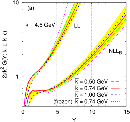
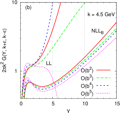
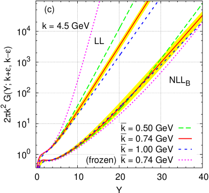
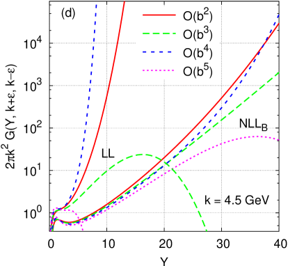
Figure 12: (a) Green’s function calculated with four different infrared regularizations of the coupling, with a renormalisation-scale band ($1/2<x_{\mu}^{2}<2$) included for reference for the ${\bar{k}}=0.74\,\,\mathrm{GeV}$ curve; (b) Green’s function calculated in the $b$-expansion, up to and including second, third, fourth and fifth orders in $b$; (c) and (d) are the same as (a) and (b) respectively but on a different scale. In all cases $\epsilon\simeq 0.1k$.

Having examined the asymptotic properties of the various infrared regularizations, we can now move on to examine the IR sensitivity of ‘perturbative’ Green’s functions. The left hand plots of Fig. 12 ((a) and (c) simply have different rapidity ranges) show $G(Y,k-\epsilon,k+\epsilon)$ for the four infrared coupling regularizations of Tab. 1. The transverse momentum $k=4.5\,\,\mathrm{GeV}$ is chosen lower than in the plots of section 4.3 in order enhance the sensitivity to the IR region. For reference we also include the uncertainty band due to renormalisation scale uncertainty. The discussion that follows will concentrate on the NLL_B results, however all the plots of Fig. 12 include also LL results, so as to illustrate the dramatically different IR sensitivity between LL and NLL_B evolution.

So let us first consider the three cutoff regularizations (NLL_B). One sees that up to $Y\simeq 30$ they give very similar results. Beyond this point, tunneling occurs (for the lowest cutoff), and the three curves start to diverge, indicating that according to this prescription the Green’s function is no longer under perturbative control.

When instead one examines the curve with an infrared-frozen coupling, one finds a result that at first sight appears paradoxical: the Green’s function is somewhat lower than with a cutoff regularization, over a wide range of $Y$ in which the cutoff regularization looks relatively insensitive to NP effects. Naively one might have expected to see little difference until the tunneling point. Our understanding of the observed behavior is that it is connected with the use of $\bar{\alpha}_{s}(q^{2})$ in Eq. (48), which causes the regularization of the coupling to affect, among other things, the virtual corrections of the BFKL equation. Having a larger infrared coupling increases the size of the (negative) virtual corrections. In situations where the Green’s function has a substantially negative second derivative (as it does over a wide range of $Y$) there is an incomplete cancellation with the real contributions (of order $1/Q^{2}$), which means that a larger infrared coupling leads to smaller preasymptotic growth of the Green’s function. This also explains why the curves with a cutoff IR coupling initially evolve more slowly for smaller values of ${\bar{k}}$.

One could also have imagined more sophisticated IR regularization schemes. For example, while maintaining an infrared-frozen coupling, one could have placed an IR cutoff on the exchanged transverse momentum $k$. We expect that this would give curves whose initial evolution is very similar to that of the IR-frozen coupling case, but whose asymptotic NP behavior is a pole, as in the cases with a cutoff on the coupling.

This confusion arising from this wide range of regularization options was in part the motivation for introducing the $b$-expansion in [23]. The $b$-expansion allows one to define a perturbative prediction in close analogy with the prescription that is implicitly contained in standard fixed-order perturbative predictions. There, one never has to specify any IR regularization. Rather, momentum integrals are implicitly carried out over a perturbative fixed-order expansion of the coupling, which is well behaved down to zero momentum. Sensitivity to non-perturbative effects then manifests itself through the appearance of renormalons (see for example the review by Beneke [50]), i.e. factorially divergent coefficients in the series expansion for one’s observable.

In a small-$x$ resummation, a pure fixed-order expansion would defeat the purpose of the resummation in the first place. However it was shown in [23] that one can expand $\log G$ in powers of the $\beta$-function coefficient $b$, and that a truncation of the resulting series maintains the advantages of small-$x$ resummation, while providing a prescription for defining purely ‘perturbative’ predictions. This is in addition to its usefulness for studying analytical properties of the running-coupling dependence of the Green’s function, as has already been exploited in Sec. 4.4.

Figs. 12b and 12d show the same Green’s function as in Figs. 12a and 12c, but in truncations of the $b$-expansion ranging from orders $b^{2}$ to $b^{5}$. One sees how all different truncations give fairly similar answers at low $Y$. But at large $Y$, the presence of the terms in $\log G$ involving additional factors of $b^{2}\alpha_{s}^{4}Y^{2}$ leads to the splaying out of the different truncations, signaling the fundamental limit of the $b$-expansion. In certain models (e.g. [26]) this is associated with the appearance of non-analyticity in $b$. It is to be noted that this large-$Y$ breakdown of the $b$-expansion is not of the renormalon type that is expected in normal perturbative series.

Figure 13: Ratios of successive coefficients of $b^{n}$ in the $b$-expansion of $\log G(Y,k-\epsilon,k+\epsilon)$ for $Y=5$.

A detailed study of the figure also reveals that even at low $Y$ the expansion is not entirely well-behaved. Indeed successive coefficients of the $b$-expansion are all of the same sign and grow quite rapidly, in a way that is suggestive of an infrared renormalon. Infrared renormalons are a factorially divergent behavior of the perturbative series whereby the $n^{\mathrm{th}}\gg 1$ order term is proportional to $(\bar{\alpha}_{s}b/p)^{n}n!$ (in simple cases). When interpreted in the language of asymptotic series, this translates to an uncertainty on the sum of the perturbative series of order $(\Lambda^{2}/Q^{2})^{p}$.

To establish whether it is renormalon behavior that we are seeing, in Fig. 13 we show ratios of successive coefficients of $b^{n}$ in the expansion of $\log G$. The fact that, over a significant range of $n$, one sees a large-$n$ behavior consistent with $(\log G)^{(n)}/(\log G)^{(n-1)}\simeq cn$, implies that it is renormalon behavior. Furthermore by examining a second value of $Q$ one can establish that $c$ itself is roughly proportional to $\bar{\alpha}_{s}$, $c\simeq 1.9\bar{\alpha}_{s}$. However the constant of proportionality, corresponding to a value of $p=\frac{asb}{c}\simeq 0.53$, is somewhat surprising, because it implies power corrections of order $(\Lambda/Q)^{2p}$, i.e. roughly $\Lambda/Q$. Naively one would have expected $p=1$ (see also [51]). This difference has yet to be understood, though it should be kept mind that significant enhancements of naively expected power-suppressed effects are known to be possible due to certain classes of resummation effects [52]. It is interesting additionally to note that the formally higher-twist non-perturbative effects that we expect for splitting functions in Sec. 5 will also turn out to scale roughly as $\Lambda/Q$ rather than $\Lambda^{2}/Q^{2}$.

Regardless of the precise reason for the unexpected scaling, it can be quite straightforwardly established that the renormalon behavior is directly connected with the use of $\bar{\alpha}_{s}(q^{2})$ in the LL part of the kernel; i.e. it has the same origin as the preasymptotic effects that arise when modifying the IR regularization of the coupling, Fig. 12a.

These preasymptotic effects are a feature of BFKL evolution that to the best of our knowledge have not been observed before. Given that they are strictly connected to the use of $\bar{\alpha}_{s}(q^{2})$, they are somewhat model dependent. However the motivations for using $\bar{\alpha}_{s}(q^{2})$ are quite strong. In particular, as we have mentioned above, this is the scale that is explicitly suggested by the form of the NLO corrections; furthermore the appearance of the transverse momentum of the emitted gluon as the scale of the coupling is a phenomenon that is well-motivated in many other contexts of QCD [53].

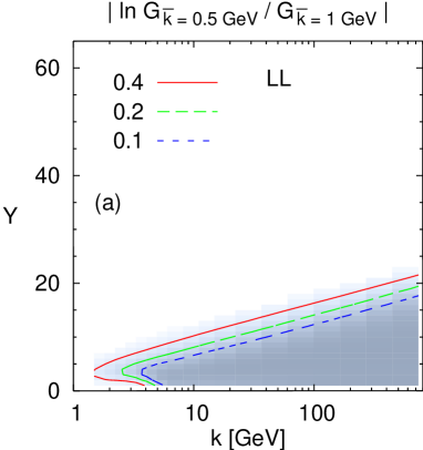
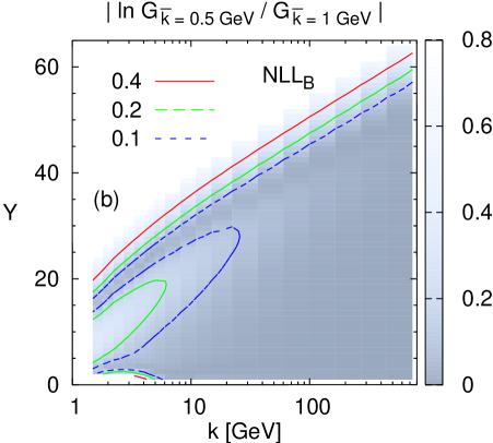
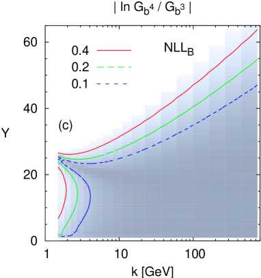
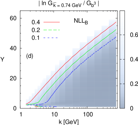
Figure 14: Contour plots showing the sensitivity of $G(Y,k-\epsilon,k+\epsilon)$ to the choice of non-perturbative regularization, obtained by examining the absolute value of the logarithm of the ratio of pairs of regularizations. Darker shades indicate insensitivity to the NP regularization, and contours have been drawn where the logarithm of the ratio is equal to $0.1$, $0.2$ and $0.4$. Plot (a) shows the result for LL evolution (with $\alpha_{s}(q)$) and two cutoff regularizations (${\bar{k}}=0.5\,\,\mathrm{GeV}$ and ${\bar{k}}=1.0\,\,\mathrm{GeV}$); (b) shows NLL_B evolution with the same pair of cutoffs; (c) shows NLL_B evolution with truncations of the $b$-expansion at orders $b^{3}$ and $b^{4}$; and (d) shows NLL_B evolution, comparing a cutoff regularization (${\bar{k}}=0.74\,\,\mathrm{GeV}$) with a $b$-expansion truncation (at order $b^{3}$).

The appearance of significant preasymptotic NP effects complicates somewhat any attempt to give a compact summary of NP limits in BFKL evolution. In their absence one might have parameterised NP effects at a given transverse scale $k$, by the rapidity at which one loses predictability for the Green’s function (e.g. [24, 23, 22]). Instead, we examine contour plots, Fig. 14, of

$$\left|\log\frac{G_{a}(Y;k-\epsilon,k+\epsilon)}{G_{b}(Y;k-\epsilon,k+\epsilon)}\right|,$$ (103)

where the subscripts $a$ and $b$ indicate the different non-perturbative treatments in the two evaluations of the Green’s function. Darker shades indicate good agreement between the two evaluations, while lighter shades indicate disagreement. Additionally, to guide the eye, we have added explicit contours where the (absolute value of the) log of the ratio is equal to $0.1$, $0.2$ and $0.4$, which for brevity we shall refer to as the $10\%$, $20\%$ and $40\%$ contours respectively.

The first plot, Fig. 14a, given for reference, shows results for LL evolution with two different IR cutoffs on the coupling ($0.5\,\,\mathrm{GeV}$ and $1\,\,\mathrm{GeV}$). Preasymptotic effects are fairly irrelevant here, in part because the asymptotic NP contributions set in quite quickly. The contours indicate a linear relation between the maximum perturbatively accessible $Y$ value, $Y_{\max}$, and $\log k$, as would be expected if this limit is due to tunneling in the Green’s function with the lower cutoff. From the simplified version of the tunneling formula [21, 22],

$$Y_{\mathrm{tunnel}}(k^{2})\simeq\frac{\log k^{2}/{\bar{k}}^{2}}{\omega_{\mathbb{P}}-\omega_{s}(k^{2})}\,,$$ (104)

we expect that for asymptotically large $k$, we should see $dY_{\max}/d\log k\simeq 2/\omega_{\mathbb{P}}\simeq 3.45$. In practice, the slope that is measured (for $k$ between $10^{3}$ and $10^{4}\,\,\mathrm{GeV}$) is about 2.7; given that the measurement region is not truly asymptotic, the $20\%$ disagreement between the two numbers is not unreasonable.

Fig. 14b uses the same pair of NP regularizations, but with NLL_B evolution. A first striking difference is the significant region (lower left-hand quadrant) in which there are preasymptotic NP effects at the $20\%$ level. This is connected with the preasymptotic effects (due to $\bar{\alpha}_{s}(q^{2})$) mentioned earlier in this section. The second important observation is that the rapidity where asymptotic non-perturbative effects become important, $Y_{\max}$, is significantly larger than for LL. But as before it is roughly consistent with a manifestation of tunneling in the Green’s function with the lower cutoff: this time the tunneling formula differs slightly from that in [21, 22], because of the presence of the kinematical constraint in the evolution, giving

$$Y_{\mathrm{tunnel,\,k.c.}}(k^{2})\simeq\frac{(1+\omega_{\mathbb{P}})\log k^{2}/{\bar{k}}^{2}}{\omega_{\mathbb{P}}-\omega_{s}(k^{2})}\,.$$ (105)

At very large $k$ one would therefore expect a slope $dY_{\max}/\log k\simeq 2(1+1/\omega_{\mathbb{P}})\simeq 6.9$. The measured slope (same $k$ range as above) is roughly $6.1$. As for LL evolution, these two results are not perfectly compatible, but given that the $k$-region is not formally asymptotic, the disagreement is not unreasonable.

As is discussed above, using different infrared regularizations is not the only way of gauging non-perturbative effects. Fig. 14c shows what happens if instead we consider two truncations of the $b$-expansion, at orders $b^{3}$ and $b^{4}$. Once again, for smaller values of $k$ there are significant preasymptotic NP effects, though the range of $k$ for which they matter is more limited. The upper (‘asymptotic’) limit on $Y$ due to NP uncertainties also behaves differently with the $b$-expansion. As was shown in [23], the $b$-expansion allows one to reach rapidities of the order of the fundamental perturbative limit [24, 25, 8, 26], $Y_{\max}\sim\log^{2}k^{2}/\Lambda^{2}$. This different parametric behavior of $Y_{\max}$, though not directly relevant for phenomenological parameter ranges, is evident from the large-$k$ curvature of the contours, and becomes even more so when going to yet larger $k$.

The plots so far have shown comparisons of pairs of IR regularizations, or pairs of $b$-expansion truncations. However if we look once again at Fig. 12, we see that the largest preasymptotic ‘NP’ differences are to be seen when comparing an IR cutoff with the $b$-expansion. Accordingly in Fig. 14d, we show contours for the ratio of Green’s functions where one is evolved with a central IR cutoff (${\bar{k}}=0.74\,\,\mathrm{GeV}$) and the other is determined by a $b^{3}$ truncation of the $b$-expansion. This is to be considered as a conservative estimate of the impact of non-perturbative effects.

In this comparison, preasymptotic NP effects are so important at lower $k$ values (below a few GeV), that one loses the ability to distinguish them clearly from asymptotic NP effects associated with tunneling or diffusion. Only for $k\gtrsim 6\,\,\mathrm{GeV}$ is one able to calculate the Green’s function over a reasonable range of rapidity (at least up to $Y=10$) with better than $20\%$ accuracy. One comes to a similar conclusion if one compares the cutoff and frozen IR coupling regularizations, as was illustrated in [32].

5 Resummed anomalous dimension and splitting function

So far, we have investigated the gluon Green’s function in the hard Pomeron regime, in which the hard scales $k^{2},k_{0}^{2}$ are of the same order, and — by the $b$-expansion method — we have isolated diffusion and running coupling effects from the non-perturbative Pomeron behavior. In the complementary regime $k^{2}\gg k_{0}^{2}$ (or $k_{0}^{2}\gg k^{2}$), the collinear properties become dominant, and the Green’s function is characterized by scaling violations and by the corresponding anomalous dimensions. The relation to non-perturbative physics changes also, because of the validity of the RG factorization property. By arguments based on the double $\gamma$-representation [16, 36, 54] or on truncated models [17, 21, 34] we can state that, for $t\gg t_{0}$,

$${\cal G}_{\omega}(k,k_{0})={\cal F}_{\omega}(k)\tilde{{\cal F}}_{\omega}(k_{0})+\rm higher\;twists\;,$$ (106)

where ${\cal F}_{\omega}$ ($\tilde{{\cal F}}_{\omega}$) is a solution of the homogeneous equation (23) which is regular for $t\rightarrow\infty$ ($t_{0}\rightarrow-\infty$). While the $t$-dependence, because of its boundary conditions, is expected to be perturbatively calculable, the $t_{0}$-dependence is sensitive to the strong-coupling region and to non-perturbative physics, but is factorized so that the standard approach of DGLAP evolution [3] can apply. We are thus entitled to define

$$\gamma_{\mathrm{res}}(\omega,t)={{\cal F}_{\omega}(t)\over g_{\omega}(t)}\;,\qquad g_{\omega}(t)=\int\frac{d\gamma}{2\pi i\gamma}\;e^{\gamma t}f_{\omega}(\gamma)\;,$$ (107)

where $f_{\omega}(\gamma)$ represents ${\cal F}_{\omega}$ in $\gamma$-space.

5.1 Resummation by $\boldsymbol{\omega}$-expansion

The analytical form of the resummed eigenfunction $f_{\omega}$ was found in [11] on the basis of the $\omega$-expansion — summarized in Sec. 2.4 — which provides the solution

$$f_{\omega}(\gamma)=\exp\left(-\frac{1}{b\omega}X_{\omega}(\gamma)\right)\;,\qquad X^{\prime}_{\omega}(\gamma)\equiv\partial_{\gamma}X_{\omega}(\gamma)\equiv\chi_{\omega}(\gamma)\;,$$ (108)

in terms of the eigenvalue function $\chi_{\omega}(\gamma)$ in Eqs. (25) and (26). Furthermore, in the “semiclassical” regime when $bt>1/\omega\gg 1$, the behavior of ${\cal F}_{\omega}(t)$ can be found from the saddle point estimate

$$b\omega t=\chi_{\omega}(\bar{\gamma}_{\omega}(t))=X^{\prime}_{\omega}(\bar{\gamma}_{\omega}(t))\;,$$ (109)

and the solution is then given by

$${\cal F}_{\omega}(t)=k^{2}{\cal F}_{\omega}(k)\sim{1\over\sqrt{-2\pi\chi^{\prime}_{\omega}(\bar{\gamma}_{\omega}(t))}}\exp\left[\int^{t}d\tau\;\bar{\gamma}_{\omega}(\tau)\right]\;,$$ (110)

where the function $\bar{\gamma}_{\omega}(t)$ satisfies the following identity

$$\bar{\gamma}_{\omega}(t)t-{1\over b\omega}X_{\omega}(\bar{\gamma})=\int^{t}\bar{\gamma}_{\omega}(\tau)d\tau\;.$$ (111)

The corresponding gluon anomalous dimension is given by [10]

$$\gamma_{\mathrm{res}}(\omega,t)=\bar{\gamma}_{\omega}(t)-\frac{b\omega}{\chi_{\omega}^{\prime}(\bar{\gamma})}\left[\frac{1}{\bar{\gamma}}+\frac{1}{2}\frac{\chi_{\omega}^{\prime\prime}(\bar{\gamma})}{\chi_{\omega}^{\prime}(\bar{\gamma})}+\dots\right]\;.$$ (112)

Recall, however, that Eq. (112) is an acceptable approximation only away from the turning point

$$\chi_{\bar{\omega}_{s}}^{\prime}\big{(}\bar{\gamma}(\bar{\omega}_{s},t)\big{)}=0\;,$$ (113)

which is a singularity of (112) with infinite fluctuations, and defines the exponent $\omega=\bar{\omega}_{s}(t)$ at anomalous dimension level.

Therefore, when $\omega$ approaches $\bar{\omega}_{s}(t)$, one can only rely on the $\gamma$-representation (107) in order to define the anomalous dimension past the turning point. This was the method followed in [11] (with the choice of scheme in Eq. (22)) in order to provide the resummed anomalous dimension and its exponent $\omega_{c}$. In the following, we refer to this this calculation as the “$\omega$-expansion” result.

5.2 Practical determination of splitting functions

Here we are more interested in providing the resummed gluon splitting function directly in $x$-space, by using the resummation scheme defined by the kernel ${\cal K}_{\omega}$ and by the corresponding Green’s function. Two methods are available to this purpose. One can exploit the $\gamma$-representation for the $t$-dependence on the gluon distribution, and define an anomalous dimension in $\omega$-space as given in Eqs. (107,108). To obtain a result in $x$-space, it is then necessary to take the inverse Mellin transform of $\gamma_{\mathrm{res}}(\omega,t)$. However our formalism for calculating the Green’s function involves a kernel with higher-order terms in $\alpha_{s}$ and this cannot be straightforwardly represented with a $\gamma$-representation, so in order to obtain a splitting function within the same ‘model’ as the Green’s function we shall need to resort to $x$-space deconvolution directly from the Green’s function, using the numerical method presented in [34]. This involves calculating the Green’s function $G(y,t,t_{0})$ and a corresponding integrated gluon density

$$xg(x,Q^{2})\equiv\int^{Q}d^{2}k\;G^{(\nu_{0}=k^{2})}(\log 1/x,k,k_{0})\;,$$ (114)

and then solving numerically the following equation for the effective splitting function $P_{\mathrm{eff}}(z,Q^{2})$,

$$\frac{dg(x,Q^{2})}{d\log Q^{2}}=\int\frac{dz}{z}\,P_{\mathrm{eff}}(z,Q^{2})\,g\left(\frac{x}{z},Q^{2}\right)\;.$$ (115)

In the limit of $Q^{2}\gg\max\{k_{0}^{2},\Lambda^{2}\}$, $P_{\mathrm{eff}}(z,Q^{2})$ should be independent of the particular choice of $k_{0}$ and of regularization of the coupling, modulo higher-twist corrections. That this is true in practice is an important verification of factorization, and provides complementarity to analytical ‘proofs’ based on simplified models.

As a first step it is interesting to check that the two methods for obtaining splitting functions are equivalent. We do this for a ‘LL$+$DGLAP’ model (which includes the kinematical constraint), namely

$$\chi_{\omega}(\gamma)=2\psi(1)-\psi(\gamma)-\psi(1-\gamma+\omega)+\omega A_{1}(\omega)\left(\frac{1}{\gamma}+\frac{1}{1-\gamma+\omega}\right)\;,$$ (116)

where the running coupling is evaluated at scale $k$. Such a model is of interest because it can be fully represented in both the $\gamma$-representation, since it has no higher-order terms in $\alpha_{s}$, and the Green’s function approach, since it is straightforwardly expressed in $k$-space. It also contains some of the typical sources of potential numerical instability (e.g. the $1/(1-z)_{+}$ term), making it a powerful ‘test-case’.

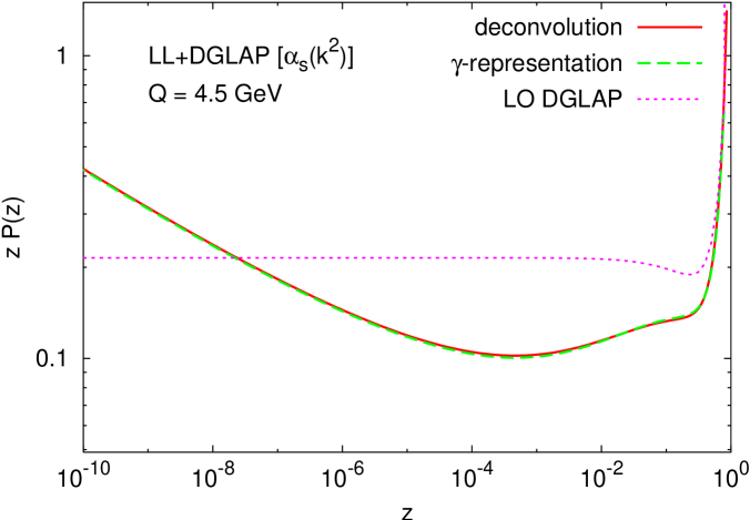
Figure 15: Small-$z$ splitting function determined by two complementary numerical methods ($\gamma$-representation and deconvolution) for the test case of the LL+DGLAP model. For reference the pure DGLAP splitting function is also shown.

Fig. 15 shows that the effective splitting functions obtained with the two methods are nearly identical. The difference between them is of the same order as the higher-twist effects that come from varying the regularization of the coupling in the deconvolution method (not shown). Also plotted is the 1-loop (LO) pure DGLAP splitting function for comparison. We note that at large $z$ one sees the standard $1/(1-z)$ behavior in all three curves.

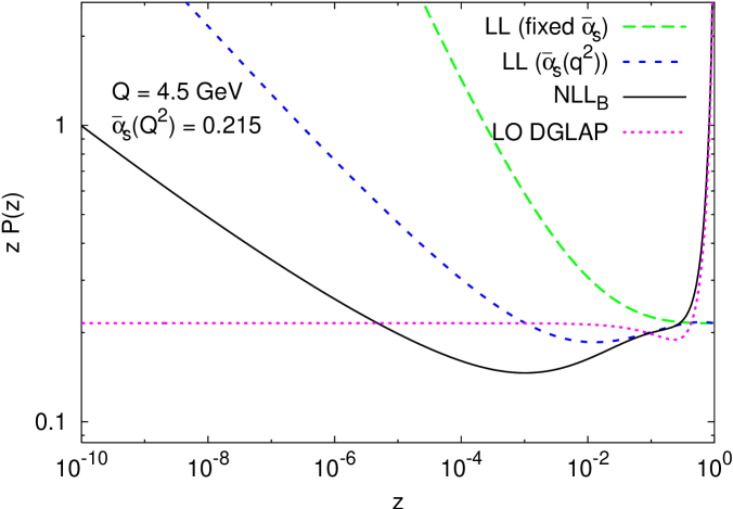
Figure 16: Small-$z$ resummed splitting function from resummation scheme B, compared to the pure 1-loop DGLAP and BFKL splitting functions (the latter with fixed and running couplings).

Having established the validity of the deconvolution approach, one can examine the effective splitting functions in the context of the full resummed kernel. We restrict our attention to scheme B, given that scheme A is not expected to obey the momentum sum rule. Since we are determining a purely gluonic splitting function we take $n_{f}=0$ in the subtracted NLL kernel, though we keep $n_{f}=4$ in occurrences of the $\beta$ function, so as to maintain a realistic running of the coupling. Switching to $n_{f}=4$ in the kernel as well has a relatively small effect, cf. Fig. 7.

Fig. 16 shows the effective splitting function for $Q=4.5\,\,\mathrm{GeV}$. It is compared to the 1-loop DGLAP splitting function, and to BFKL splitting functions obtained in the pure LL approximation with fixed ($\bar{\alpha}_{s}\equiv\bar{\alpha}_{s}(Q^{2})\simeq 0.215$) and running ($\bar{\alpha}_{s}(q^{2})$) couplings.

It is perhaps of interest to discuss first the two LL curves. As can be seen from the figure (and as has been discussed extensively elsewhere [11, 34, 13, 36, 37]), running coupling effects alone give strong modifications relative to the fixed-coupling LL splitting function. There is a taming of the asymptotic behavior: the cut at $\omega_{s}=4\log 2\bar{\alpha}_{s}\simeq 0.60$ is converted to a series of poles, the leading one being at $\omega_{c}\simeq 0.25$, with the difference $\omega_{s}-\omega_{c}$ formally of order $\bar{\alpha}_{s}^{5/3}$ [47, 48, 11]. The running of the coupling also leads to preasymptotic effects, in particular it is associated with a dip at moderately small $z$. Similar features have been discussed by other authors as well, though the details differ: in [13] the running as $\bar{\alpha}_{s}(q^{2})$ is fully implemented only through to NLL order. In [36, 37] the coupling runs as $\bar{\alpha}_{s}(k^{2})$ (a NLL difference) and furthermore the use of the Airy approximation in the evaluation of the expressions analogous to our Eqs. (107,108) means that their results do not quite correspond to an exact solution of Eqs. (2) and (115).

From the discussion in section 4 for the Green’s function, one expects a further strong suppression of the asymptotic growth when going from LL to NLL_B— for example (for $b(n_{f}=4)$) $\omega_{s}$ goes from $0.60$ to $0.27$. However because of non-linearities (and the compensation of some double counting), the correction to the splitting function from the combination of running coupling and NLL_B effects is weaker than would be expected from a simple linear combination of the two separate effects. Indeed the final running-coupling, NLL_B result for $\omega_{c}$ with $\bar{\alpha}_{s}(Q^{2})=0.215$ is $\omega_{c}\simeq 0.18$. The preasymptotic dip, to which we return below, is also modified in the NLL_B resummation, becoming somewhat deeper (about $30\%$ of $\bar{\alpha}_{s}$) and moving to smaller $z$ ($\sim 10^{-3}$).

Other important characteristics of the splitting function extracted in scheme B are the large-$z$ behavior, which coincides with the expected LO DGLAP result and the value of its first moment ($\omega=1$): the scheme has been constructed such that for fixed coupling, the effective characteristic function satisfies $\bar{\alpha}_{s}\chi_{\mathrm{eff}}(\gamma=0,\bar{\alpha}_{s})=1$. At fixed-coupling, duality arguments [12] then automatically lead to the splitting function having a zero first moment (to within higher-twist corrections), i.e. validity of the momentum sum rule. More generally, for running coupling we expect the momentum sum-rule to hold because at $\omega=1$ the kernel is free of leading-twist poles. It is therefore interesting to observe that after full inclusion of the IR regularized running coupling, and our rather sophisticated deconvolution approach, the numerically derived splitting function of Fig. 16 does indeed have a first moment which is zero, to within a few parts in $10^{4}$. (We have not so far succeeded in establishing the detailed origin of this small departure from zero, though it may well be a higher-twist contribution).

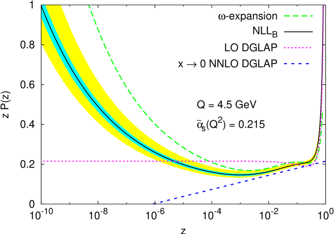
Figure 17: The small-$z$ resummed splitting function for ${\bar{k}}=0.74\,\,\mathrm{GeV}$ and $x_{\mu}=1$ together with renormalisation scale and IR-regularization uncertainties; the inner band is due to the variation of ${\bar{k}}$ between $0.5\,\,\mathrm{GeV}$ and $1.0\,\,\mathrm{GeV}$, while the outer band comes from varying the renormalisation scale in the range $1/2<x_{\mu}^{2}<2$. Also shown are the splitting function obtained with the $\omega$-expansion [11] (calculated with a $\beta_{0}$ corresponding to $n_{f}=4$), the LO DGLAP $P_{gg}$ and the known small-$x$ parts of the NNLO DGLAP $P_{gg}$.

Given the large difference between the original fixed-coupling LL splitting function and the running coupling scheme B result, it is important to establish the order of magnitude of potential higher-order and non-perturbative uncertainties. This question is addressed in figure 17, where the scheme B splitting function is shown together with two uncertainty bands. The inner band is that associated with the variation of the infrared cutoff ${\bar{k}}$ between $0.5$ and $1\,\,\mathrm{GeV}$, indicating a modest non-perturbative uncertainty.

The outer band shows the effect of varying $x_{\mu}$ in the range $0.5<x_{\mu}^{2}<2$ (a range commonly used for fully inclusive quantities). This should give an estimate of the importance of potential higher-order corrections. One sees that the main features of the splitting function are stable, though at small $z$ the uncertainty grows because different renormalisation scales lead to slightly different $\omega_{c}$ powers. Another way of investigating higher-order uncertainties is to consider the $\omega$-expansion of [11] — here recalculated with the same $n_{f}$ convention as used for scheme B ($n_{f}=4$ in the $\beta$-function and $n_{f}=0$ in the rest of the kernel) and transformed to $z$-space. We recall that the $\omega$-expansion is based on the same assumptions as scheme B, namely LL+NLL BFKL and the requirement of correct LO DGLAP limits. From fig. 17 one sees that down to $z\sim 10^{-3}$ it agrees with scheme B to within the renormalisation scale uncertainties. Below, the NLL_B and $\omega$-expansion curves move further apart, essentially because their $\omega_{c}$ values ($0.18$ and $0.20$ respectively) differ by more than would be expected based on the $x_{\mu}$ variation. This suggests that for future phenomenological purposes, in the very small-$z$ region one might wish to consider the effects of a larger range of $x_{\mu}$ variation.

An aspect of the splitting function that deserves more comment is the dip at moderately small $z$. A priori one may wonder about its origin and indeed whether it might not be some form of artefact of our resummation procedure. To help resolve the issue fig. 17 also shows the known small-$z$ part of the NNL DGLAP splitting function (for $n_{f}=0$):

$$zP_{gg}(z)=\bar{\alpha}_{s}+B\bar{\alpha}_{s}^{3}\log\frac{1}{z}\,,\qquad B=-\frac{395}{108}+\frac{\zeta(3)}{2}+\frac{11\pi^{2}}{72}\simeq-1.549\,.$$ (117)

One sees that the initial decrease of the scheme-B splitting function corresponds closely to the decrease of the pure NNL DGLAP splitting function, associated with the $B\bar{\alpha}_{s}^{3}\log 1/z$ term. At a certain point however small-$z$ resummation effects set in and the scheme-B structure function starts to rise, giving the characteristic dip structure. The fact that the initial decrease of the full $P_{gg}$ is correlated with an exactly determined (NLL$x$) piece of the NNL DGLAP splitting function suggests that the dip structure is a true feature of the small-$z$ splitting function. This belief is reinforced by the observed robustness of the dip structure under renormalisation scale and resummation scheme changes (though the depth of the dip is subject to some degree of uncertainty).

An interesting question concerns the impact of the dip on fits to parton distributions. Calculations in a (partially) RGI LL model [43] whose effective splitting function also has a dip, suggest that it is not incompatible with the available structure function data. Ref. [13] mentions work in progress on fits involving a resummed splitting function with a dip (actually considerably deeper than ours), but detailed results have yet to be presented. It should of course be kept in mind that so far we have only presented results for purely gluonic problems — phenomenological studies will additionally require a treatment of the quark sector.

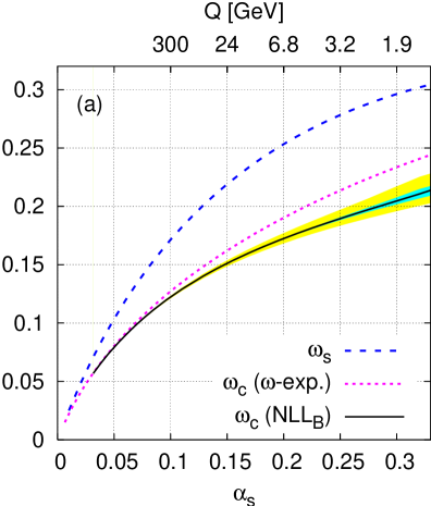
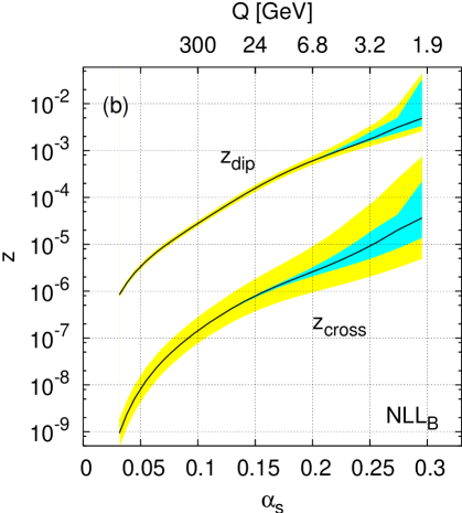
Figure 18: (a) the small-$z$ exponent, $\omega_{c}$ of the effective BFKL splitting function in resummation scheme B, compared to the previous $\omega$-expansion result, and to the Green’s function $\omega_{s}$ as determined in section 4.4 (NLL_B); (b) the position ($z_{\mathrm{dip}}$) of the small-$z$ minimum of the splitting function and the point ($z_{\mathrm{cross}}$) below which the resummed splitting function becomes larger than the 1-loop DGLAP $P_{gg}$. The inner and outer bands have the same meaning as in Fig. 17.

To close off this section, we examine how certain properties of the effective splitting function depend on the coupling $\alpha_{s}$, Fig. 18. One quantity of interest is the formal small-$z$ exponent, $\omega_{c}$, shown in the left-hand plot, together with uncertainty bands from varying the IR regularization and the renormalisation scale. One sees that at small $\alpha_{s}$, regularization uncertainties very quickly become negligible, in accord with their expected higher-twist nature, while renormalisation-scale uncertainties decrease much more slowly with $\alpha_{s}$. Also shown, for comparison, are curves for $\omega_{c}$ in the $\omega$-expansion (quite similar to scheme B) and a reproduction of the results of section 4.4 for $\omega_{s}$ to first order in $b$ (here shown with $n_{f}=4$ in $b$, whereas in section 4.4 $n_{f}$ was uniformly 0).

Given the late onset of the small-$z$ power growth, other interesting quantities are the position of the dip, $z_{\mathrm{dip}}$, and the point where the effective splitting function becomes larger than the plain 1-loop DGLAP splitting function (always defined with $x_{\mu}=1$), $z_{\mathrm{cross}}$. Both quantities are shown as a function of $\alpha_{s}$ in the right-hand plot of Fig. 18. As one would perhaps expect, as one decreases $\alpha_{s}$, one has to go to progressively smaller values of $z$ before the BFKL increase of the splitting function becomes visible. In this plot too we note the contrast between regularization uncertainties which vanish rapidly with $Q$ and renormalisation scale uncertainties which vary much more slowly with $Q$.

6 Inclusion of impact factors

For a realistic calculation of a physical cross section, high energy factorization requires that one specify also the impact factors characterizing the external probes (Sec. 2.1). The impact factors are known in the LL approximation for a variety of physical processes [27, 28], and also in the NLL approximation for virtual photons [31] and for forward jet production [30]. However, the corresponding expressions are quite involved and still to be implemented in numerical algorithms. Furthermore, their accuracy stops at the first non-trivial order in $\alpha_{s}$.

The purpose of this section is to show how the resummed scheme for $\tilde{{\cal G}}_{\omega}$ can be extended to the corresponding impact factors $\tilde{h}$’s by incorporating subleading corrections due to 1) phase-space and threshold effects and 2) leading log collinear singularities. The inclusion of the exact NL impact factor expressions [30, 31] is left to a future investigation.

6.1 Phase space and threshold effects

Let’s first consider deep inelastic scattering $\gamma^{*}(q)+p\to hadrons$ in the high energy regime $\nu\equiv 2pq\equiv Q^{2}/x_{B}\gg Q^{2}$. According to the analysis presented in Ref. [27] we can factorize the LL contribution to the $\gamma^{*}p$ cross section in the form

$$\sigma^{\gamma^{*}p}(\nu,Q)=\int\frac{d\nu_{1}}{\nu_{1}}\,\frac{d\nu_{2}}{\nu_{2}}\,\frac{d^{2}{\boldsymbol{k}}}{{\boldsymbol{k}}^{2}}\;h(\nu_{1},Q,{\boldsymbol{k}})\,f(\nu_{2},{\boldsymbol{k}})\,\Theta\left(\nu-\frac{\nu_{1}\nu_{2}}{{\boldsymbol{k}}^{2}}\right)\;.$$ (118)

$h$ and $f$ represent the off-shell $\gamma^{*}\mathsf{g}^{*}$ and $\mathsf{g}^{*}p$ cross sections in which the virtual gluon has a particular polarization. The $\Theta$ function indicates the threshold condition to be satisfied in the multi-Regge kinematics (MRK) $\nu\gg\nu_{1},\nu_{2}\gg Q^{2},{\boldsymbol{k}}^{2}$ by the invariants defined in Fig. 19a.

This threshold condition expresses the fact that the longitudinal part of the momentum transfer is small with respect to its longitudinal part (consistency constraint [41, 42, 43]). In fact, in a frame where the momenta $p$ and $q$ have no transverse component, one has

$$q =q^{\prime}-xp$$ (119a)

$$k =-\bar{z}q^{\prime}+zp+{\boldsymbol{k}}\;:\quad q^{\prime}\cdot{\boldsymbol{k}}=0=p\cdot{\boldsymbol{k}}\;.$$ (119b)

In the last equation, one has to remember the euclidean nature of ${\boldsymbol{k}}$: $-k_{\mu}k^{\mu}=z\bar{z}\nu+{\boldsymbol{k}}^{2}$. The relations among invariants and Sudakov parameters are given by

$$z =\frac{1}{\nu}\left(\nu_{1}-\frac{Q^{2}}{\nu}\nu_{2}\right)$$ (120a)

$$\bar{z} =\frac{\nu_{2}}{\nu}$$ (120b)

$$|k_{\mu}k^{\mu}| ={\boldsymbol{k}}^{2}+\frac{\nu_{2}}{\nu}\left(\nu_{1}-\frac{Q^{2}}{\nu}\nu_{2}\right)\;.$$ (120c)

MRK implies $\nu_{1}\gg Q^{2}\nu_{2}/\nu$, hence Eqs. (120a,120c) can be approximated by

$$z \simeq\frac{\nu_{1}}{\nu}$$ (121a)

$$|k_{\mu}k^{\mu}| \simeq{\boldsymbol{k}}^{2}+\frac{\nu_{1}\nu_{2}}{\nu}\geq\frac{\nu_{1}\nu_{2}}{\nu}\;.$$ (121b)

Therefore, if ${\boldsymbol{k}}^{2}$ were replaced by $|k_{\mu}k^{\mu}|$, the $\Theta$ function would represent just a phase space threshold. As it stands, it yields the consistency condition that the virtuality of the gluon is essentially transverse, that is

$${\boldsymbol{k}}^{2}\simeq|k_{\mu}k^{\mu}|\geq\frac{\nu_{1}\nu_{2}}{\nu}\;,$$ (122)

i.e., the condition in Eq. (118). The additional thresholds $(q+k)^{2}\simeq\nu_{1}-Q^{2}+{\boldsymbol{k}}^{2}>0$ and $(p-k)^{2}\simeq\nu_{2}-{\boldsymbol{k}}^{2}>0$ — ensuring the final state particles to be in the forward light cone — are implicitly contained in $h$ and $f$ respectively.

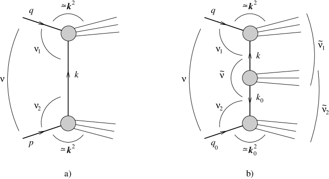
Figure 19: Kinematic diagrams for: a) deep inelastic scattering; b) $\gamma^{*}\gamma^{*}$ cross section. The variables correspond to (2 times) the scalar product of the corresponding momenta, e.g., $\nu_{1}=2q\cdot k$, $\nu_{2}=2p\cdot(-k)=2q_{0}\cdot k_{0}$, $\tilde{\nu}_{2}=2q_{0}\cdot(-k)$ etc..

According to Eq. (121a), we can rewrite Eq. (118) as

$$\sigma^{\gamma^{*}p}(\nu,Q) =\int_{Q^{2}}^{\nu}\frac{d\nu_{1}}{\nu_{1}}\,\frac{d^{2}{\boldsymbol{k}}}{{\boldsymbol{k}}^{2}}\;h\left(\frac{Q^{2}}{\nu_{1}},Q,{\boldsymbol{k}}\right){\cal F}\left(\frac{\nu_{1}}{\nu},{\boldsymbol{k}}\right)$$ (123)

$$=\int_{x_{B}}^{1}\frac{dz}{z}\frac{d^{2}{\boldsymbol{k}}}{{\boldsymbol{k}}^{2}}\;h\left(\frac{x_{B}}{z},Q,{\boldsymbol{k}}\right){\cal F}(z,{\boldsymbol{k}})$$ (124)

in terms of the unintegrated gluon density

$${\cal F}(z,{\boldsymbol{k}})=\int\frac{d\nu_{2}}{\nu_{2}}\;f(\nu_{2},{\boldsymbol{k}})\,\Theta\left(\nu-\frac{\nu_{1}\nu_{2}}{{\boldsymbol{k}}^{2}}\right)\;.$$ (125)

Eq. (124) is the well known factorization formula for DIS which we present for later convenience also as a convolution in the invariant “energy variable” $\nu_{1}$ (Eq. (123)).

Taking the Mellin transform w.r.t. $\nu/Q^{2}=x_{B}^{-1}$, yields the simpler structure

$$\sigma^{\gamma^{*}p}_{\omega}(Q)=\int\frac{d^{2}{\boldsymbol{k}}}{{\boldsymbol{k}}^{2}}\;h_{\omega}(Q,{\boldsymbol{k}}){\cal F}_{\omega}({\boldsymbol{k}})\;,$$ (126)

in terms of Mellin transforms of the original factors.

We remark that the LL behavior of $\sigma^{\gamma^{*}p}$ is determined by the leading (rightmost) singularity $\omega=\omega_{\mathbb{P}}(\alpha_{s})\stackrel{{\scriptstyle\alpha_{s}\to 0}}{{\longrightarrow}}0$ of ${\cal F}_{\omega}$ in the $\omega$-plane, while $h_{\omega}=h_{0}+{\cal O}(\omega)$ contributes at LL level only through its zero-moment $h_{0}$. This amounts to integrating $h(\nu_{1},Q,{\boldsymbol{k}})$ in $\nu_{1}$ regardless of the $\nu_{1}$-dependence in ${\cal F}$ and identifying in ${\cal F}$: $\nu_{1}=Q^{2}$, i.e., $z=x_{B}$. This shows that the details of the phase space effects, in particular those at threshold — evidently ignored in the approximation $h_{\omega}\simeq h_{0}$ just mentioned — appear only as a NL contribution. On the other hand, they are expected to be important when the total energy $\nu$ has moderately high values. Therefore, the $\omega$-dependent formulation of impact factors is suitable to describe subleading effects coming from the proper treatment of the phase space.

This applies also to the double ${\boldsymbol{k}}$-factorization formula describing the high energy $\gamma^{*}\gamma^{*}$ cross section: in the MRK $\nu\gg\tilde{\nu_{1}},\tilde{\nu_{2}}\gg\tilde{\nu},\nu_{1},\nu_{2}\gg Q^{2},Q_{0}^{2},{\boldsymbol{k}}^{2},{\boldsymbol{k}}_{0}^{2}$ the threshold condition (121b) can be applied to any $2\to 2$ subdiagram of Fig. 19b:

$$\tilde{\nu}_{1}>\frac{\tilde{\nu}\nu_{1}}{{\boldsymbol{k}}^{2}}\;,\qquad\tilde{\nu}_{2}>\frac{\tilde{\nu}\nu_{2}}{{\boldsymbol{k}}_{0}^{2}}\;,\qquad\nu>\frac{\nu_{1}\tilde{\nu}_{2}}{{\boldsymbol{k}}^{2}}\;,\qquad\nu>\frac{\nu_{2}\tilde{\nu}_{1}}{{\boldsymbol{k}}_{0}^{2}}\quad\Longrightarrow\quad\nu>\frac{\tilde{\nu}\nu_{1}\nu_{2}}{{\boldsymbol{k}}^{2}{\boldsymbol{k}}_{0}^{2}}>\frac{\nu_{1}\nu_{2}}{|{\boldsymbol{k}}||{\boldsymbol{k}}_{0}|}\;.$$ (127)

The last inequality (obtained by using $\tilde{\nu}>|{\boldsymbol{k}}||{\boldsymbol{k}}_{0}|$) shows that the boundary of phase space can be very simply described by the combination $\nu_{1}\nu_{2}/(\nu|{\boldsymbol{k}}||{\boldsymbol{k}}_{0}|)$. This suggests that we write the high energy cross section for photons of polarization $A$ and $B$ ($A,B=T,L$) as

$$\sigma^{AB}(\nu,Q^{2},Q_{0}^{2})=\int \frac{d\nu_{1}}{\nu_{1}}\,\frac{d\nu_{2}}{\nu_{2}}\,\frac{d^{2}{\boldsymbol{k}}}{{\boldsymbol{k}}^{2}}\,\frac{d^{2}{\boldsymbol{k}}_{0}}{{\boldsymbol{k}}_{0}^{2}}$$ (128)

$$h^{A}(\nu_{1},Q,{\boldsymbol{k}})\,{\cal G}\left(\frac{\nu{\boldsymbol{k}}^{2}{\boldsymbol{k}}_{0}^{2}}{\nu_{1}\nu_{2}},{\boldsymbol{k}},{\boldsymbol{k}}_{0}\right)\,h^{B}(\nu_{2},Q_{0},{\boldsymbol{k}}_{0})\,$$

where ${\cal G}$, representing the $\mathsf{g}^{*}\mathsf{g}^{*}$ off shell cross section integrated in the “invariant mass” $\tilde{\nu}$, contains the total energy dependence and is constrained by the last of the threshold conditions (127).

Eq. (128) is just equivalent to the ${\boldsymbol{k}}$-factorization formula (1) in energy space, because the convolution in the energy variables can be diagonalized by means of the following Mellin transforms:

$$\sigma^{AB}_{\omega}(Q,Q_{0}) =\int_{QQ_{0}}^{\infty}\frac{d\nu}{\nu}\left(\frac{QQ_{0}}{\nu}\right)^{\omega}\sigma^{AB}(\nu,Q,Q_{0})$$ (129a)

$$h_{\omega}(Q,{\boldsymbol{k}}) =\int_{Q|{\boldsymbol{k}}|}^{\infty}\frac{d\nu_{1}}{\nu_{1}}\left(\frac{Q|{\boldsymbol{k}}|}{\nu_{1}}\right)^{\omega}h(\nu_{1},Q,{\boldsymbol{k}})$$ (129b)

$${\cal G}_{\omega}({\boldsymbol{k}},{\boldsymbol{k}}_{0}) =\int_{0}^{1}\frac{du}{u}\;u^{\omega}{\cal G}\left(\frac{|{\boldsymbol{k}}||{\boldsymbol{k}}_{0}|}{u},{\boldsymbol{k}},{\boldsymbol{k}}_{0}\right)\;,\qquad u=\frac{\nu_{1}\nu_{2}}{\nu|{\boldsymbol{k}}||{\boldsymbol{k}}_{0}|}\;.$$ (129c)

In fact, by using the equality

$$\frac{QQ_{0}}{\nu}=\frac{Q|{\boldsymbol{k}}|}{\nu_{1}}\;\frac{\nu_{1}\nu_{2}}{\nu|{\boldsymbol{k}}||{\boldsymbol{k}}_{0}|}\;\frac{Q_{0}|{\boldsymbol{k}}_{0}|}{\nu_{2}}$$ (130)

and the thresholds (122) and (127), we obtain

$$\sigma^{AB}_{\omega}(Q,Q_{0})=\int\frac{d^{2}{\boldsymbol{k}}}{{\boldsymbol{k}}^{2}}\,\frac{d^{2}{\boldsymbol{k}}_{0}}{{\boldsymbol{k}}_{0}^{2}}\;h^{A}_{\omega}(Q,{\boldsymbol{k}})\,{\cal G}_{\omega}({\boldsymbol{k}},{\boldsymbol{k}}_{0})h^{B}_{\omega}(Q_{0},{\boldsymbol{k}}_{0})\;.$$ (131)

The choice of a symmetric energy scale $\nu_{0}=QQ_{0}$ leads naturally to symmetric energy scales for the individual factors $h_{\omega}$ and ${\cal G}_{\omega}$, as one can see in Eqs. (129).

The lesson is that even in the double high energy factorization formula, a single Mellin variable $\omega$ allows one to treat in a proper way the kinematics of the process, in particular the threshold effects. This motivates our choice to use $\omega$-dependent impact factors and kernel.

6.2 Collinear resummation of impact factors

Additional subleading contributions to $\sigma^{\gamma^{*}\gamma^{*}}$ not taken into account in the Green’s function are higher order perturbative corrections to the impact factors. Here we want to analyze the additional corrections which are important in the collinear limits $Q\gg Q_{0}$ and $Q\ll Q_{0}$. In order to keep the discussion as simple as possible, we analyze only the fixed coupling ($b=0$) case.

In Sec. 2.4 we have shown that we can replace the original RG improved Green’s function ${\cal G}$ of Eq. (2) with $\tilde{\cal G}$ of Eq. (30) — the latter being defined in term of the modified kernel (32) — up to NNLL differences. Correspondingly one should define impact factors $\tilde{h}$’s which provide the same cross section in the new scheme.

We begin by considering Eq. (131) with LO impact factors and with the effective Green’s function $\tilde{\cal G}$. With fixed coupling, both the impact factor and the Green’s function are scale invariant, and the cross section can be given the integral representation

$$\sigma^{AB}_{\omega}(Q,Q_{0}) =\frac{\pi}{QQ_{0}}\int\frac{d\gamma}{2\pi i}\left(\frac{Q_{0}^{2}}{Q^{2}}\right)^{\gamma-\frac{1}{2}}\sigma_{\omega}(\gamma)$$ (132)

$$\sigma_{\omega}(\gamma) \simeq\tilde{h}_{\omega}^{A}(\gamma)\,\tilde{{\cal G}}_{\omega}(\gamma)\,\tilde{h}_{\omega}^{B}(1-\gamma)$$ (133)

where we have introduced the Mellin transforms

$$h_{\omega}(\gamma) \equiv\int\frac{d{\boldsymbol{k}}^{2}}{{\boldsymbol{k}}^{2}}\left(\frac{{\boldsymbol{k}}^{2}}{Q^{2}}\right)^{\gamma-1}h_{\omega}(Q,{\boldsymbol{k}})$$ (134a)

$${\cal G}_{\omega}(\gamma) \equiv\int d^{2}{\boldsymbol{k}}_{0}\left(\frac{{\boldsymbol{k}}_{0}^{2}}{{\boldsymbol{k}}^{2}}\right)^{\gamma-1}{\cal G}_{\omega}({\boldsymbol{k}},{\boldsymbol{k}}_{0})$$ (134b)

We shall now compare the collinear behavior of (133) to that predicted for the total cross section in order to find the NLL corrections in $\tilde{h}^{A}$ at collinear level. In $\gamma$-space the formulation of collinear factorization becomes particularly simple in the fixed coupling case, and can be stated as follows: the leading $\log Q^{2}/Q_{0}^{2}$ contribution ($Q\gg Q_{0}$) — corresponding to the behavior at $\gamma\simeq-{\textstyle\frac{\omega}{2}}$ for the Mellin transform — to the photon-photon cross section at order $\alpha^{2}\alpha_{s}^{n}$ is given by

$$\sigma_{\omega}^{AB}(\gamma)\sim\frac{4\pi\alpha V_{\omega}^{A}}{\gamma+{\textstyle\frac{\omega}{2}}}\sum_{\text{\sf a}_{1}\cdots\text{\sf a}_{n-1}=\mathsf{q},\mathsf{g}}\frac{\gamma_{\omega}^{\mathsf{q}\text{\sf a}_{1}}}{\gamma+{\textstyle\frac{\omega}{2}}}\;\frac{\gamma_{\omega}^{\text{\sf a}_{1}\text{\sf a}_{2}}}{\gamma+{\textstyle\frac{\omega}{2}}}\cdots\frac{\gamma_{\omega}^{\text{\sf a}_{n-1}\mathsf{q}}}{\gamma+{\textstyle\frac{\omega}{2}}}\;\frac{\gamma_{\omega}^{\mathsf{q}\gamma}V_{\omega}^{B}}{\gamma+{\textstyle\frac{\omega}{2}}}$$ (135)

in terms of the one-loop anomalous dimensions $\gamma_{\omega}^{\text{\sf b}\text{\sf a}}$ describing the “probability” of the $\text{\sf a}\to\text{\sf b}$ splitting, and of additional “photon-vertex factors” $V_{\omega}^{j}$ distinguishing the polarization of the corresponding photon:

$$V_{\omega}^{T}=1\;,\qquad V_{\omega}^{L}=\left(\gamma+{\textstyle\frac{\omega}{2}}\right)\big{(}1+{\cal O}(\omega)\big{)}\;.$$ (136)

If we restrict our analysis to gluon emission only, beside the two $\mathsf{q}\bar{\mathsf{q}}$ pairs coupling to the two photons, in Eq. (135) all $\text{\sf a}_{i}$ but two are just gluons. A further approximation, valid in the high energy limit, is to neglect collinear gluon emissions between two quarks belonging to the same loop. In fact, this amounts to neglecting $\mathsf{q}\to\mathsf{q}$ splittings which are proportional to $\gamma_{\omega}^{\mathsf{q}\mathsf{q}}=0+{\cal O}(\omega)$. Therefore, $\text{\sf a}_{1}=\text{\sf a}_{n-1}=\mathsf{q}$ and $\text{\sf a}_{2}\cdots\text{\sf a}_{n-2}=\mathsf{g}$.

In order to find the collinear behavior of the resummed impact factors, we have to compare Eq. (135) with the ${\boldsymbol{k}}$-factorization formula (131). The collinear behavior of the RGI kernel (33) at $b=0$ is simply

$$\tilde{\chi}_{\omega}(\gamma)\simeq\bar{\alpha}_{s}(\chi_{0}^{\omega}+\omega\chi_{\mathrm{c}}^{\omega})\sim\frac{\omega\gamma_{\omega}^{\mathsf{g}\mathsf{g}}}{\gamma+{\textstyle\frac{\omega}{2}}}$$ (137)

This determines the collinear behavior of the RGI Green’s function

$$\tilde{{\cal G}}_{\omega}(\gamma)\sim[\omega-\tilde{\chi}_{\omega}(\gamma)]^{-1}=\frac{1}{\omega}\sum_{n=0}^{\infty}\left(\frac{\gamma_{\omega}^{\mathsf{g}\mathsf{g}}}{\gamma+{\textstyle\frac{\omega}{2}}}\right)^{n}$$ (138)

The collinear behavior of the LO impact factors with exact kinematics [55] is

$$h_{\omega}^{T(0)}(\gamma) =h_{\omega}^{T(0)}(1-\gamma)\sim 2\alpha\sqrt{N_{c}^{2}-1}\gamma_{\omega}^{\mathsf{q}\mathsf{g}}\frac{1}{(\gamma+{\textstyle\frac{\omega}{2}})^{2}}$$ (139a)

$$h_{\omega}^{L(0)}(\gamma) =h_{\omega}^{L(0)}(1-\gamma)\sim 2\alpha\sqrt{N_{c}^{2}-1}\gamma_{\omega}^{\mathsf{q}\mathsf{g}}\frac{1}{\gamma+{\textstyle\frac{\omega}{2}}}\,\frac{1+\omega}{1+\frac{3}{4}\omega+\frac{1}{4}\omega^{2}}\;.$$ (139b)

Using the relation

$$\gamma_{\omega}^{\mathsf{q}\gamma}=\frac{\alpha}{\alpha_{s}}2N_{c}\gamma_{\omega}^{\mathsf{q}\mathsf{g}}\;,$$ (140)

the Mellin transform of the cross section with LO impact factors assumes the form

$$\left.\sigma_{\omega}^{AB}(\gamma)\right|_{\text{LO imp.fac.}} \simeq h_{\omega}^{A(0)}(\gamma)\tilde{{\cal G}}_{\omega}(\gamma)h_{\omega}^{B(0)}(1-\gamma)$$

$$\sim\frac{4\pi\alpha V_{\omega}^{A}}{\gamma+{\textstyle\frac{\omega}{2}}}\;\frac{\gamma_{\omega}^{\mathsf{q}\mathsf{g}}}{\gamma+{\textstyle\frac{\omega}{2}}}\;\sum_{n=0}^{\infty}\left(\frac{\gamma_{\omega}^{\mathsf{g}\mathsf{g}}}{\gamma+{\textstyle\frac{\omega}{2}}}\right)^{n}\;\frac{\gamma_{\omega}^{\mathsf{g}\mathsf{q},\mathrm{sing}}}{\gamma+{\textstyle\frac{\omega}{2}}}\;\frac{\gamma_{\omega}^{\mathsf{q}\gamma}V_{\omega}^{B}}{\gamma+{\textstyle\frac{\omega}{2}}}$$ (141)

having decomposed the anomalous dimensions relative to the $\mathsf{q}\to\mathsf{g}$ splitting in a singular $\propto 1/\omega$ and a non-singular part:

$$\gamma_{\omega}^{\mathsf{g}\mathsf{q}}=\frac{C_{F}}{C_{A}}\left[\frac{1}{\omega}+B(\omega)\right]\equiv\gamma_{\omega}^{\mathsf{g}\mathsf{q},\mathrm{sing}}+\gamma_{\omega}^{\mathsf{g}\mathsf{q},\mathrm{n.s.}}$$ (142)

We can see from Eq. (141) that the structure of Eq. (135) is reproduced, but in the $\mathsf{q}\to\mathsf{g}$ splitting we are taking into account only the singular part of the anomalous dimension.

This is not a surprise, because the LO impact factors are by definition coupled to the Green’s function via a high energy gluon exchange, i.e., a singular splitting. Surprising enough is the fact that, using the effective Green’s function, it suffices to use upper impact factor at LO only, in order to obtain the correct collinear singularities on its side. The reason is that the additional factor

$$(1-\bar{\alpha}_{s}K^{\omega}_{\mathrm{c}})^{-1}=\sum_{n=0}^{\infty}(\bar{\alpha}_{s}K^{\omega}_{\mathrm{c}})^{n}$$ (143)

stemming from the resolvent of $\tilde{\cal K}_{\omega}$ (see Eq. (30)) provides exactly the non-singular splittings needed to build up the collinear corrections of the upper impact factor to all orders, in the collinear ordering $Q\gg k$.

On the other hand, the full expression (135) contains the correction factor $1+\omega B(\omega)$ w.r.t. Eq. (141), due to the full $\mathsf{q}\to\mathsf{g}$ anomalous dimension (142). This factor is attributed to the lower impact factor in the collinear region $k_{0}\gg Q_{0}$, so that we can set, at NLL level,

$$\tilde{h}_{\omega}^{B}(1-\gamma) =h_{\omega}^{B(0)}(1-\gamma)+\omega B(\omega)h_{\omega R}^{B(0)}(1-\gamma)$$

$$\simeq\tilde{h}_{\omega}^{B(0)}(1-\gamma)\left[1+\bar{\alpha}_{s}\frac{B(\omega)}{\gamma+{\textstyle\frac{\omega}{2}}}\right]+\text{NNLL}\;,$$ (144)

where the additional term shows right-hand singularities only in the $1-\gamma$ variable (i.e., $\Re(1-\gamma)>1/2$).

Analyzing the opposite ordering $Q_{0}\gg Q$ — thus the leading right-hand singularities in the variable $\gamma$ (i.e., $\Re(\gamma)>1/2$) — yields the modification of the upper impact factor

$$\tilde{h}_{\omega}^{A}(\gamma)=h_{\omega}^{A(0)}(\gamma)\left[1+\bar{\alpha}_{s}\frac{B(\omega)}{1-\gamma+{\textstyle\frac{\omega}{2}}}\right]+\text{NNLL}\;,$$ (145)

which differs from Eq. (144) by the replacements $A\leftrightarrow B$ and $\gamma\leftrightarrow 1-\gamma$.

In conclusion, the high energy cross section can be factorized in the product of the Green’s function $\tilde{{\cal G}}_{\omega}$ and impact factors $\tilde{h}$ as follows:

$$\sigma^{AB}_{\omega}(Q,Q_{0})=\int\frac{d^{2}{\boldsymbol{k}}}{{\boldsymbol{k}}^{2}}\,\frac{d^{2}{\boldsymbol{k}}_{0}}{{\boldsymbol{k}}_{0}^{2}}\;\tilde{h}^{A}_{\omega}(Q,{\boldsymbol{k}})\,\tilde{{\cal G}}_{\omega}({\boldsymbol{k}},{\boldsymbol{k}}_{0})\tilde{h}^{B}_{\omega}(Q_{0},{\boldsymbol{k}}_{0})\;.$$ (146)

Such a factorization formula includes the full one-loop anomalous dimensions to all orders, the NLL contributions of the Green’s function and the NLL phase space effects. Still missing are the running coupling effects and the subleading collinear NLL corrections to the impact factors. The former could be easily incorporated in the collinear limit on the basis of a straightforward generalization of Eq. (141). The latter can be included from the known results [31] on the basis of the change of scheme discussed below.

6.3 Next-to-leading impact factors in the $\boldsymbol{\omega}$-independent formulation

Here we wish to relate the $\omega$-dependent formulation of ${\boldsymbol{k}}$-factorization and of BFKL evolution used so far, to the more conventional next-to-leading log expansion of the cross section. We shall see that this involves a redefinition of NLL impact factors which is somewhat ambiguous, and considerably complicates their collinear structure. For the sake of simplicity, we shall provide the relation in the frozen $\alpha_{s}$ limit.

We have already encountered the operator relation of the $\omega$-dependent Green’s function to the BFKL one up to NLL order. According to Eq. (39) we have

$$\tilde{{\cal G}}_{\omega}\simeq[1-\bar{\alpha}_{s}(K_{0}^{1}+K^{0}_{\mathrm{c}})]^{-1}\big{[}\omega-\bar{\alpha}_{s}(K_{0}+\bar{\alpha}_{s}K_{1}+{\cal O}(\alpha_{s}^{2})\big{]}^{-1}\;,$$ (147)

which differs from the pure BFKL-type expansion by the operator factor ${\cal H}=[1-\bar{\alpha}_{s}(K_{0}^{1}+K^{0}_{\mathrm{c}})]^{-1}$. The latter originates from the $\omega$-shift (expanded to first order in $\omega$) and from the collinear behavior. It was first introduced in [5] where it was shown to provide energy-independent terms, which compensate the symmetrical scale choice $s_{0}=kk_{0}$, so as to provide the effective energy scale $s_{>}=\max(k^{2},k_{0}^{2})$ for the Green’s function. On the other hand, the complete cross section includes the impact factors $\tilde{h}$’s according to Eqs. (146) and (145), and should be consistent with the NLL parameterisation

$$\sigma^{AB}(\nu,Q,Q_{0}) =\int\frac{d\omega}{2\pi i}\left(\frac{\nu}{QQ_{0}}\right)^{\omega}\frac{d^{2}{\boldsymbol{k}}}{{\boldsymbol{k}}^{2}}\,\frac{d^{2}{\boldsymbol{k}}_{0}}{{\boldsymbol{k}}_{0}^{2}}\;\big{(}h^{A(0)}(Q,{\boldsymbol{k}})+\alpha_{s}h^{A(1)}(Q,{\boldsymbol{k}})\big{)}$$ (148)

$$\quad\times\langle{\boldsymbol{k}}|[\omega-\bar{\alpha}_{s}(K_{0}+\bar{\alpha}_{s}K_{1})]^{-1}|{\boldsymbol{k}}_{0}\rangle\big{(}h^{B(0)}(Q_{0},{\boldsymbol{k}}_{0})+\alpha_{s}h^{B(1)}(Q_{0},{\boldsymbol{k}}_{0})\big{)}\;.$$

In order to compare Eq. (146) with (147) and (148), we see that the factor ${\cal H}$ has to be incorporated in the impact factors. We can do that, given the eigenvalue function ${\cal H}(\gamma)={\cal H}(1-\gamma)$, by defining some function ${\cal H}_{L}(\gamma)$ such that ${\cal H}(\gamma)={\cal H}_{L}(\gamma){\cal H}_{L}(1-\gamma)$, and by assigning factor ${\cal H}_{L}(\gamma)$ (${\cal H}_{L}(1-\gamma)$) to impact factor $A$ ($B$). This decomposition is not unique, however, and each solution for ${\cal H}_{L}$ corresponds to a choice of ${\boldsymbol{k}}$-factorization scheme [5] in the subtraction of the leading term at NLL level in perturbation theory. Furthermore, the $\omega$-dependence should be expanded in the $\tilde{h}$’s also. In $\gamma$-space we have

$$\tilde{h}_{\omega}^{A}=h^{(0)A}_{\omega=0}+\omega\left.\partial_{\omega}h^{(0)A}_{\omega}\right|_{\omega=0}+\bar{\alpha}_{s}\tilde{h}^{(1)A}_{\omega=0}\simeq h^{(0)A}_{\omega=0}+\bar{\alpha}_{s}\left[\left.\partial_{\omega}h^{(0)A}_{\omega}\right|_{\omega=0}\chi_{0}+\tilde{h}^{(1)A}_{\omega=0}\right]\;,$$ (149)

where in the last line we have exploited that the factor $(\omega-\bar{\alpha}_{s}\chi_{0})$ eliminates the high energy part of the cross section.

On the other hand, at NL level the factorization of the ${\cal H}$ factor is achieved by setting ${\cal H}_{L}(\gamma)=1+\bar{\alpha}_{s}H(\gamma)+{\cal O}(\bar{\alpha}_{s}^{2})$, with

$$H(\gamma)+H(1-\gamma)=\chi_{0}^{1}(\gamma)+\chi_{\mathrm{c}}^{0}(\gamma)\simeq-\frac{1}{2}\left[\frac{1}{\gamma^{2}}+\frac{1}{(1-\gamma)^{2}}\right]+A(0)\left[\frac{1}{\gamma}+\frac{1}{(1-\gamma)}\right]$$ (150)

Therefore, the NL contribution to the impact factor in the $\omega$-independent expansion becomes

$$h^{(1)A}(\gamma)=h^{(0)A}_{\omega=0}(\gamma)H(\gamma)+\left.\partial_{\omega}h^{(0)A}_{\omega}(\gamma)\right|_{\omega=0}\chi_{0}(\gamma)+\tilde{h}^{(1)A}_{\omega=0}(\gamma)\;.$$ (151)

We see from Eq. (151) that the first two terms both generate higher order singularities which — e.g., for $A=T$ — are of type $1/\gamma^{4}$ and $1/(1-\gamma)^{4}$, and come from the $\omega$-derivative and from multiplication by the singular $H$ term. In order to extract the dynamically interesting correction $\tilde{h}^{(1)A}$ from a perturbative calculation of $h^{(1)A}$, one has to subtract both terms from $h^{(1)A}$, by a proper choice of $H$, corresponding to a proper factorization scheme.

7 Discussion

In this paper we have presented a formulation of the resummed small-$x$ equation based on the renormalisation group constraints. The equation presented here embodies correctly the LL and NLL BFKL kernels as well as LL DGLAP evolution. The new equation is very close to the formulation proposed previously [11], the main difference being the treatment of the collinear terms, which are here treated as $\omega$-dependent terms of the leading kernel. The advantage of the small-$x$ equation proposed here is that it shows simple collinear poles only and is defined directly in $k$ and rapidity space thus making it easy to study the full gluon Green’s function rather than just its high-energy exponents. Therefore, after inclusion of the impact factors, it can be used in a straightforward way for phenomenological applications to processes with two hard scales.

In our numerical analysis we have obtained the solutions to this equation in the case of fixed and running coupling, we have studied the energy dependence of the Green’s function both for comparable scales and in the collinear limit and we have extracted the corresponding splitting function.

The analysis of the Green’s function has confirmed the fact [21, 26] that the hard Pomeron exponent $\omega_{s}(\alpha_{s})$ parametrizes only a transient rapidity dependence of the gluon density, to be modified by non-linear diffusion corrections at perturbative level and — beyond some critical rapidity — by the non-perturbative Pomeron behavior. Nevertheless, subleading resummation effects not only decrease and stabilize $\omega_{s}$ itself (Fig. 11), but basically weaken the non-perturbative Pomeron and considerably increase the range of validity of the perturbative behavior (Fig. 14) by 10–20 units in rapidity compared to leading log expectations. Therefore, we are encouraged to trust the resummed perturbative predictions for next generation accelerators [32].

We have provided resummed results for the gluon splitting function also. This is a purely perturbative quantity, as has been verified from its definition as the logarithmic derivative of the gluon density, by checking collinear factorization for $Q\gg Q_{0}$. Here resummation effects stabilize the (oscillating) $\log s$ hierarchy, and cause a soft departure from the DGLAP result, showing a shallow dip in the moderate-$x$ region, followed by the expected power increase in the very small-$x$ region, characterized by the splitting function exponent $\omega_{c}(\alpha_{s})$.

Let us now comment in a little more detail on some interesting features of our results. For the high-energy exponents, this work confirms the picture of Ref. [11]. The resummed Green’s function exponent $\omega_{s}(\alpha_{s})$ turns out to be numerically similar to $\alpha_{s}$ for relevant values of $\alpha_{s}$ (Fig. 11). This exponent is closely related to the saddle point singularity discussed in [11], but cannot really be identified with it, due to the presence of diffusion corrections to the exponent with the same rapidity dependence. For this reason, the extraction of $\omega_{s}$ requires the subtraction of the leading $Y^{3}$ diffusion term, which turns out to be small compared to leading log expectations. On the other hand, the splitting function exponent $\omega_{c}(\alpha_{s})$ is substantially below $\omega_{s}$ — by about 0.1 for typical $\alpha_{s}$ — due to well-known running coupling effects.

In addition, we find here interesting preasymptotic effects in the energy dependence of the gluon density at comparable scales. In particular, the growth of the NLL_B resummed density is delayed up to rapidities of order $Y\simeq 4$ for $\alpha_{s}\simeq 0.2$. It is also worth commenting on the expectations for the onset of perturbative non-linear (saturation) effects in the evolution. These become relevant when the Green’s function is of order $1/\alpha_{s}$ [56]. For our reference scales ($k_{t}\simeq 5$ GeV and $\alpha_{s}\simeq 0.2$), this translates to $Y$ of order $15$, i.e. close to the kinematic limit of LHC.

A special comment is needed for the splitting function’s dip in the moderate-$x$ region. It is at most a 30% effect with respect to the DGLAP value for $\alpha_{s}\simeq 0.2$, spread over several orders of magnitude in $x$. It is therefore a shallow dip, associated with several subleading effects (notably the small-$z$ terms of the NNLO DGLAP splitting function), and it signals a quite moderate departure from pure LO DGLAP evolution. Considering this result and the values of $\omega_{c}(\alpha_{s})$ just mentioned, the overall picture is that our resummed predictions are much closer to low order results than naively expected. In turn, this may provide an explanation for the apparent success of low order evolution to fit HERA data, despite the size of the effective coupling $\alpha_{s}(Q^{2})\log(1/x)$.

In order to compare the present results to experimental data, we need to include the physical impact factors for two–scale processes, and quark evolution for DIS processes. Both issues are well studied. For quarks we can follow [54, 11] and for impact factors we have shown here how to incorporate the collinear resummation (in the frozen coupling limit). We recall that the NL contribution to the impact factors depends on the formulation of evolution kernel (e.g. $\omega$-dependent or independent). In our $\omega$-dependent approach, the impact factors have a simple collinear behavior due to the $\omega$ shift of leading poles. The relation to the more conventional $\omega$-independent calculations [31] is given by the subtraction procedure outlined in Sec. 6.3.

On the whole, we have presented here a unified description of small-$x$ deep inelastic processes, applicable to both the structure function regime and to the $\gamma^{*}\gamma^{*}$ kinematics. Resummed results push the validity of perturbative QCD towards higher energies and give perhaps a preliminary explanation of the cross-sections’ apparent smoothness in the small-$x$ regime despite the occurrence, in their description, of large perturbative coefficients and various strong-coupling phenomena.

Appendix A Computation of eigenvalues and projections

We give here some details of the calculation of the kernel eigenvalues and Mellin transforms which are needed for Secs. 3.2 and 4.4.

Let us start from the computation of the eigenvalues of the kernel

$$\frac{1}{\boldsymbol{q}^{2}}\left(\frac{\boldsymbol{q}^{2}}{{\boldsymbol{k}}^{2}}\right)^{\lambda}-\frac{1}{\lambda}\delta^{2}(\boldsymbol{q})\equiv H_{\lambda}({\boldsymbol{k}},{\boldsymbol{k}}^{\prime})\;,$$ (152)

possibly multiplied by the $\omega$-shifting factor $\left(\frac{k_{<}}{k_{>}}\right)^{\omega}$, in order to obtain the kernel of Eq. (88) of the text. Such kernels are closely related to the regularized form of the leading BFKL kernel (with or without consistency constraint), by possibly including powers of $\log q^{2}$ due to the running coupling.

Note first that, denoting by $\chi^{[\lambda]}(\gamma)$ the eigenvalue function of $H_{\lambda}$, the shifted kernel $\left(\frac{k_{<}}{k_{>}}\right)^{\omega}H_{\lambda}$ has eigenvalues

$$\chi_{L}^{[\lambda]}\Big{(}\gamma+{\textstyle\frac{\omega}{2}}\Big{)}+\chi_{R}^{[\lambda]}\Big{(}\gamma-{\textstyle\frac{\omega}{2}}\Big{)}\;,$$ (153)

where the left (right) projections of $f(\gamma)$ are defined by

$$f_{L,R}(\gamma)\equiv\pm\int_{\Re\gamma^{\prime}\lessgtr\Re\gamma}\frac{d\gamma^{\prime}}{2\pi i}\;\frac{f(\gamma^{\prime})}{\gamma-\gamma^{\prime}}=\sum_{\begin{matrix}\gamma_{n}\leq 0\\ \gamma_{n}\geq 1\end{matrix}}\frac{f(\gamma_{n})}{\gamma-\gamma_{n}}\;,$$ (154)

with the upper (lower) determination of signs and conditions. Note that the last expression holds in the particular case of simple pole singularities in the left (right) $\gamma$-plane. In fact, such eigenvalues are found by the Fourier transform

$$\int dt^{\prime}\int\frac{d\gamma^{\prime}}{2\pi i}\;\chi^{[\lambda]}(\gamma^{\prime})e^{\gamma^{\prime}(t-t^{\prime})}\left[e^{-{\textstyle\frac{\omega}{2}}(t-t^{\prime})}\Theta(t-t^{\prime})+e^{-{\textstyle\frac{\omega}{2}}(t^{\prime}-t)}\Theta(t^{\prime}-t)\right]e^{\gamma(t^{\prime}-t)}$$

$$=\int_{0}^{\infty}d\tau\int_{{\textstyle\frac{1}{2}}-i\infty}^{{\textstyle\frac{1}{2}}+i\infty}\frac{d\gamma^{\prime}}{2\pi i}\;\chi^{[\lambda]}(\gamma^{\prime})\left[e^{(-\gamma-{\textstyle\frac{\omega}{2}}+\gamma^{\prime})\tau}+e^{(\gamma-{\textstyle\frac{\omega}{2}}-\gamma^{\prime})\tau}\right]\;.$$ (155)

In this equation, the $\gamma^{\prime}$ integral can be displaced to the left (right) of $\gamma+{\textstyle\frac{\omega}{2}}$ ($\gamma-{\textstyle\frac{\omega}{2}}$) in the first (second) term in the r.h.s.. By then performing the $\tau$-integral in its convergence region we obtain, by the definition (154), the result (153).

We then compute $\chi^{[\lambda]}(\gamma)$ itself by applying the kernel $H_{\lambda}$ to the test function $({\boldsymbol{k}}^{\prime}{}^{2})^{\gamma-1}$. By using then known integral

$$\int\frac{d^{2}{\boldsymbol{k}}^{\prime}}{\pi}\;\frac{1}{({\boldsymbol{k}}^{\prime 2})^{1-\gamma}[({\boldsymbol{k}}-{\boldsymbol{k}}^{\prime})^{2}]^{1-\lambda}}=\frac{\Gamma(\lambda)\Gamma(\gamma)\Gamma(1-\gamma-\lambda)}{\Gamma(1-\lambda)\Gamma(1-\gamma)\Gamma(\gamma+\lambda)}$$ (156)

and the representation

$$\frac{\Gamma(z+\epsilon)}{\Gamma(z)}=\exp\left[\epsilon\psi(z)+\frac{1}{2!}\epsilon^{2}\psi^{\prime}(z)+\frac{1}{3!}\epsilon^{3}\psi^{\prime\prime}(z)+\cdots\right]\;,$$ (157)

we obtain [$\chi_{0}(\gamma)\equiv 2\psi(1)-\psi(\gamma)-\psi(1-\gamma)$]

$$\chi^{[\lambda]}(\gamma) =\frac{1}{\lambda}\left(\frac{\Gamma(\lambda)\Gamma(\gamma)\Gamma(1-\gamma-\lambda)}{\Gamma(1-\lambda)\Gamma(1-\gamma)\Gamma(\gamma+\lambda)}-1\right)$$ (158)

$$\simeq\frac{1}{\lambda}\left\{\exp\left[\lambda\chi_{0}(\gamma)+\frac{1}{2}\lambda^{2}\chi_{0}^{\prime}(\gamma)+\frac{1}{6}\lambda^{3}\left(2\psi^{\prime\prime}(1)-\psi^{\prime\prime}(\gamma)-\psi^{\prime\prime}(1-\gamma)\right)+\cdots\right]-1\right\}$$

which proves Eq. (89) of the text. Note the cancellation of the $\lambda=0$ singularity between real emission and virtual term.

By expanding (158) in $\lambda$ we obtain, at order $\lambda^{0}$, the BFKL eigenvalue, at order $\lambda$ the eigenvalue of the running coupling kernel of Eq. (38), and so on. The corresponding kernels with consistency constraint are obtained by shifting the left/right projections of Eqs. (153) and (154).

The simplest left/right projections are based on the formulas

$$\chi_{0L}(\gamma) =\chi_{0R}(1-\gamma)=\psi(1)-\psi(\gamma)=\sum_{n=0}^{\infty}\frac{1-\gamma}{(1+n)(\gamma+n)}=\sum_{n=0}^{\infty}\left(\frac{1}{\gamma+n}-\frac{1}{1+n}\right)$$ (159)

$$-\chi^{\prime}_{0L}(\gamma) =\psi^{\prime}(\gamma)=\sum_{n=0}^{\infty}\frac{1}{(\gamma+n)^{2}}\;,\quad\psi^{\prime}(\gamma)+\psi^{\prime}(1-\gamma)=\frac{\pi^{2}}{\sin^{2}(\pi\gamma)}\;.$$ (160)

For the shifted running coupling kernel we need $[\chi_{0}^{2}+\chi_{0}^{\prime}]_{L}$ and thus $[\chi_{0}^{2}]_{L}(\gamma)$. Since $\chi_{0}=\chi_{0L}+\chi_{0R}$ we obtain

$$[\chi_{0}^{2}]_{L}(\gamma)=[\chi_{0L}(\gamma)]^{2}+2[\chi_{0L}(\gamma)\chi_{0L}(1-\gamma)]_{L}\;.$$ (161)

The last term has simple poles in the l.h.s., so that by Eq. (154) it is expressed by a sum over residues as

$$2[\chi_{0L}(\gamma)\chi_{0L}(1-\gamma)]_{L}=\chi_{0L}^{2}({\textstyle\frac{1}{2}})+2\sum_{n=1}^{\infty}\frac{\chi_{0L}(1+n)({\textstyle\frac{1}{2}}-\gamma)}{({\textstyle\frac{1}{2}}+n)(\gamma+n)}\;,$$ (162)

where a subtraction at $\gamma={\textstyle\frac{1}{2}}$ has been performed to make the series convergent, and $\chi_{0L}({\textstyle\frac{1}{2}})={\textstyle\frac{1}{2}}\chi_{0}({\textstyle\frac{1}{2}})=2\log 2$.

The series in the r.h.s. (with simple poles) is expressed as a combination of $[\chi_{0L}]^{2}$ (which has simple and double poles) and of $\psi^{\prime}$ (with double poles only), as follows:

$$2[\chi_{0L}(\gamma)\chi_{0L}(1-\gamma)]_{L} =[\chi_{0L}(\gamma)]^{2}-\psi^{\prime}(\gamma)+\frac{\pi^{2}}{2}$$ (163a)

$$2[\chi_{0L}(\gamma)\chi_{0L}(1-\gamma)]_{R} =[\chi_{0L}(1-\gamma)]^{2}-\psi^{\prime}(1-\gamma)+\frac{\pi^{2}}{2}\;.$$ (163b)

Eqs. (163) can be proved by checking residues and values at $\gamma={\textstyle\frac{1}{2}}$ of l.h.s. and r.h.s. and coincides with Eq. (93) of the text.

Finally, the left/right projections of $\tilde{\chi}_{1}(\gamma)$ as given in Eq. (41) are computed on the basis of Fourier transforms of the type (155) by splitting the $\tau$ integration into the $]\infty,0]$ ($[0,-\infty[$) intervals for the L (R) projection. The result is

$$\tilde{\chi}_{1L}(\gamma) =\frac{1}{2}\psi^{\prime\prime}(\gamma)+\chi_{0L}(\gamma)\left[\psi^{\prime}(\gamma)-A_{1}(0)\left(\frac{1}{\gamma}+\frac{1}{1-\gamma}\right)+\frac{67}{36}-\frac{\pi^{2}}{12}-\frac{5}{18}\frac{n_{f}}{N_{c}}\right]$$ (164)

$$\quad+\Pi(\gamma)-\Phi_{L}(\gamma)+\frac{\pi^{2}}{8}\left[\psi\Big{(}\frac{1+\gamma}{2}\Big{)}-\psi\Big{(}\frac{\gamma}{2}\Big{)}\right]+\frac{3}{4}\zeta(3)$$

$$\quad+\frac{1}{32}\left\{-3M(\gamma)+\left(1+\frac{n_{f}}{N_{c}^{3}}\right)\left[\frac{1}{4}\left(\frac{1}{\gamma^{2}}-\frac{1}{(1-\gamma)^{2}}\right)-\frac{1}{2}\left(\frac{1}{\gamma}-\frac{1}{1-\gamma}\right)\right.\right.$$

$$\qquad\qquad\qquad\qquad\qquad\qquad\qquad\;\left.\left.+\frac{1}{32}\Big{(}M(\gamma+1)+M(\gamma-1)\Big{)}-\frac{11}{16}M(\gamma)\right]\right\}\;,$$

where

$$\Pi(\gamma) \equiv\int_{0}^{1}dt\;t^{\gamma-1}\frac{{\mathrm{Li}_{2}}(1)-{\mathrm{Li}_{2}}(t)}{1-t}=\sum_{n=0}^{\infty}\frac{\psi^{\prime}(n+1)}{n+\gamma}$$ (165)

$$\Phi_{L}(\gamma) \equiv\sum_{n=0}^{\infty}(-1)^{n}\frac{\psi(n+1+\gamma)-\psi(1)}{(n+\gamma)^{2}}$$ (166)

$$M(\gamma) \equiv\frac{1}{\gamma-{\textstyle\frac{1}{2}}}\left[\psi^{\prime}\Big{(}\frac{1+\gamma}{2}\Big{)}-\psi^{\prime}\Big{(}\frac{\gamma}{2}\Big{)}+\psi^{\prime}\Big{(}\frac{1}{4}\Big{)}-\psi^{\prime}\Big{(}\frac{3}{4}\Big{)}\right]\;.$$ (167)

The corresponding expressions for $\tilde{\chi}_{1}$ in scheme A (Eq. (60)) and in scheme B (Eq. (62)) are respectively

$$\tilde{\chi}_{1L}^{\omega,\mathbf{A}}(\gamma) =\tilde{\chi}_{1L}(\gamma)+C(0)[\chi_{0L}(\gamma+{\textstyle\frac{\omega}{2}})-\chi_{0L}(\gamma)]$$ (168)

$$\tilde{\chi}_{1L}^{\omega,\mathbf{B}}(\gamma) =\tilde{\chi}_{1L}(\gamma)+C(\omega)[1+\omega A_{1}(\omega)]\frac{1}{\gamma+{\textstyle\frac{\omega}{2}}}-C(0)\frac{1}{\gamma}\;.$$ (169)

References

-
[1]
L.N. Lipatov, Sov. J. Nucl. Phys. 23 (1976) 338;
E.A. Kuraev, L.N. Lipatov and V.S. Fadin, Sov. Phys. JETP 45 (1977) 199;
I.I. Balitsky and L.N. Lipatov, Sov. J. Nucl. Phys. 28 (1978) 338. -
[2]
ZEUS Collab., M. Derrick et al., Phys. Lett. B 316 (1993) 412;
ZEUS Collab., M. Derrick et al., Z. Phys. C 65 (1995) 379;
ZEUS Collab., M. Derrick et al., Z. Phys. C 72 (1996) 399;
ZEUS Collab., S. Chekanov et al., Eur. Phys. J. C 21 (2001) 443;
H1 Collab., I. Abt et al., Nucl. Phys. B 407 (1993) 515;
H1 Collab., S. Aid et al., Nucl. Phys. B 470 (1996) 3;
H1 Collab., C. Adloff et al., Nucl. Phys. B 497 (1997) 3;
H1 Collab., C. Adloff et al., Eur. Phys. J. C 13 (2000) 609;
H1 Collab., C. Adloff et al., Eur. Phys. J. C 21 (2001) 33.
-
[3]
V.N. Gribov and L.N. Lipatov, Sov. J. Nucl. Phys. 15 (1972) 438;
G. Altarelli and G. Parisi, Nucl. Phys. B 126 (1977) 298;
Yu.L. Dokshitzer, Sov. Phys. JETP 46 (1977) 641. -
[4]
V.S. Fadin, M.I. Kotsky and R. Fiore, Phys. Lett. B 359 (1995) 181;
V.S. Fadin, M.I. Kotsky and L.N. Lipatov, BUDKERINP-96-92, hep-ph/9704267; V.S. Fadin, R. Fiore, A. Flachi and M.I. Kotsky, Phys. Lett. B 422 (1998) 287;
V.S. Fadin and L.N. Lipatov, Phys. Lett. B 429 (1998) 127.
- [5] G. Camici and M. Ciafaloni, Phys. Lett. B 386 (1996) 341; Phys. Lett. B 412 (1997) 396, [Erratum-ibid.Phys. Lett. B 417 (1997) 390]; Phys. Lett. B 430 (1998) 349.
-
[6]
J. Blumlein and A. Vogt, Phys. Rev. D 57 (1998) 1;Phys. Rev. D 58 (1998) 014020;
J. Blumlein, V. Ravindran and W.L. van Neerven,Phys. Rev. D 58 (1998) 091502. - [7] D.A. Ross, Phys. Lett. B 431 (1998) 161.
- [8] E.M. Levin, Nucl. Phys. B 453 (1995) 303; Nucl. Phys. B 545 (1999) 481.
- [9] G.P. Salam, JHEP 9807 (1998) 19.
- [10] M. Ciafaloni and D. Colferai, Phys. Lett. B 452 (1999) 372.
- [11] M. Ciafaloni, D. Colferai and G.P. Salam, Phys. Rev. D 60 (1999) 114036.
- [12] G. Altarelli, R.D. Ball and S. Forte, Nucl. Phys. B 575 (2000) 313; Nucl. Phys. B 599 (2001) 383.
- [13] R.S. Thorne, Phys. Rev. D 64 (2001) 074005; Phys. Lett. B 474 (2000) 372.
- [14] C.R. Schmidt, Phys. Rev. D 60 (1999) 074003; MSUHEP-90416, hep-ph/9904368.
- [15] S.J. Brodsky, V.S. Fadin, V.T. Kim, L.N. Lipatov and G.B. Pivovarov, JETP Lett. 70 (1999) 155.
- [16] J. Kwieciński, Z. Phys. C 29 (1985) 561; J.C. Collins and J. Kwieciński Nucl. Phys. B 316 (1989) 307.
- [17] L.N. Lipatov, Sov. Phys. JETP 63 (1986) 904.
- [18] G. Camici and M. Ciafaloni, Phys. Lett. B 395 (1997) 118.
- [19] A.H. Mueller and H. Navelet, Nucl. Phys. B 282 (1987) 727.
- [20] For example see S.J. Brodsky, F. Hautmann and D.E. Soper, Phys. Rev. D 56 (1997) 6957.
- [21] M. Ciafaloni, D. Colferai and G. P. Salam, JHEP 9910 (1999) 017.
- [22] M. Ciafaloni, D. Colferai, G.P. Salam and A.M. Staśto, Phys. Lett. B 541 (2002) 314.
- [23] M. Ciafaloni, D. Colferai, G.P. Salam and A.M. Staśto, Phys. Rev. D 66 (2002) 054014.
- [24] Y.V. Kovchegov and A.H. Mueller, Phys. Lett. B 439 (1998) 428.
- [25] N. Armesto, J. Bartels and M.A. Braun, Phys. Lett. B 442 (1998) 459.
- [26] M. Ciafaloni, A.H. Mueller and M. Taiuti, Nucl. Phys. B 616 (2001) 349.
- [27] S. Catani, M. Ciafaloni and F. Hautmann, Phys. Lett. B 242 (1990) 97; Nucl. Phys. B 366 (1991) 657;
-
[28]
M. Ciafaloni, Phys. Lett. B 429 (1998) 363;
M. Ciafaloni and D. Colferai Nucl. Phys. B 538 (1999) 187;
M. Ciafaloni and G. Rodrigo, JHEP 0005 (2000) 042. - [29] V.S. Fadin and A.D. Martin, Phys. Rev. D 60 (1999) 114008.
- [30] J. Bartels, D. Colferai and G.P. Vacca, Eur. Phys. J. C 24 (2002) 83; hep-ph/0206290.
-
[31]
J. Bartels, S. Gieseke and C.-F. Qiao, Phys. Rev. D 63 (2001) 056014;
Erratum-ibid. Phys. Rev. D 65 (2002) 079902;
J. Bartels, S. Gieseke and A. Kyrieleis, Phys. Rev. D 65 (2002) 014006;
J. Bartels, D. Colferai, S. Gieseke and A. Kyrieleis, Phys. Rev. D 66 (2002) 094017. - [32] M. Ciafaloni, D. Colferai, G.P. Salam and A.M. Staśto, hep-ph/0305254.
- [33] G. Bottazzi, G. Marchesini, G.P. Salam and M. Scorletti, Nucl. Phys. B 505 (1997) 366.
- [34] M. Ciafaloni, D. Colferai and G.P. Salam, JHEP 0007 (2000) 054.
- [35] G.P. Salam, Acta Phys. Polon. B 30 (1999) 3679.
- [36] G. Altarelli, R.D. Ball and S. Forte, Nucl. Phys. B 621 (2002) 359.
- [37] G. Altarelli, R. D. Ball and S. Forte,
-
[38]
A.H. Mueller, Nucl. Phys. B (Proc. Suppl.) 18C (1990) 125;
A.H. Mueller, J. Phys. G17 (1991) 1443;
J. Bartels, A. De Roeck and M. Loewe, Z. Phys. C 54 (1992) 635;
J. Kwieciński, A.D. Martin and P.J. Sutton, Phys. Rev. D 46 (1992) 921;
J. Kwiecinski, S. C. Lang and A. D. Martin, Phys. Rev. D 55 (1997) 1273. - [39] B. Andersson, G. Gustafson, H. Kharraziha and J. Samuelsson, Z. Phys. C 71 (1996) 613.
- [40] J. Kwieciński, A. D. Martin and P. J. Sutton, Z. Phys. C 71 (1996) 585.
- [41] M. Ciafaloni, Nucl. Phys. B 296 (1988) 49.
- [42] B. Andersson, G. Gustafson and J. Samuelsson, Nucl. Phys. B 467 (1996) 443.
- [43] J. Kwieciński, A. D. Martin and A.M. Staśto, Phys. Rev. D 56 (1997) 3991.
- [44] M. Ciafaloni, Phys. Lett. B 356 (1995) 74.
- [45] J. R. Andersen and A. Sabio Vera, hep-ph/0305236.
- [46] B. Abbott et al. [D0 Collaboration], Phys. Rev. Lett. 84 (2000) 5722.
- [47] R.E. Hancock and D.A. Ross, Nucl. Phys. B 383 (1992) 575; Nucl. Phys. B 394 (1993) 200.
- [48] J.R. Forshaw and D.A. Ross, Perturbative QCD and the Pomeron, Cambridge University Press, 1997.
- [49] A. Donnachie and P.V. Landshoff, Phys. Lett. B 437 (1998) 408.
- [50] M. Beneke, Phys. Rep. 317 (1999) 1.
- [51] F. Hautmann, Phys. Rev. Lett. 80 (1998) 3198.
- [52] Y.L. Dokshitzer, G. Marchesini and B.R. Webber, JHEP 9907 (1999) 012.
-
[53]
A. Bassetto, M. Ciafaloni and G. Marchesini, Phys. Rep. 100 (1983) 201;
Y. L. Dokshitzer and D.V. Shirkov, Z. Phys. C 67 (1995) 449. - [54] G. Camici and M. Ciafaloni, Nucl. Phys. B 496 (1997) 305; Erratum-ibid. Nucl. Phys. B 607 (2001) 431.
- [55] A. Bialas, H. Navelet and R. Peschanski, Nucl. Phys. B 603 (218) 2001.
- [56] L. V. Gribov, E. M. Levin and M. G. Ryskin, Phys. Rep. 100 (1983) 1.