One-loop finite potential for $N-2$ scalars from $N$ quantum fields

Abstract

We study the one-loop effective potential induced from quantum fluctuation of a finite number of fields. A series expansion in terms of the modified Bessel functions is useful to evaluate the one-loop effective potential. We find that at most $N-2$ scalars parameterize the one-loop finite potential and the explicit parameterization is shown. The structure of the potential for $N=4$ is investigated as the simplest case. The implication of the model is discussed.

I Introduction

In general field theories, quadratic and logarithmic divergence appears in the derivation of one-loop quantum corrections to some physical parameters. We need a cut-off scale to regularize the loop integration. This leads to a cut-off scale dependence of the one-loop potential and the source of the hierarchy problem in the unification theories.

In higher-dimensional theory, it is said that the one-loop finite potential for extra-components of gauge field as scalars can be obtained from (an infinite number of four-dimensional) quantum fields without supersymmetry. The symmetry breaking mechanism according to such a potential is called as the Hosotani mechanism Hos . The reason why the finite potential is possible, in spite of the worse degree of divergence in higher dimensions, is that the divergent part is independent of the scalar degrees of freedom ABQ ; GNS .

Recently a new type of theory, which is known as deconstruction ACG , attracts much attention. A number of copies of a four-dimensional theory linked by a new set of fields can be viewed as a single theory. The resulting theory may be almost equivalent to a higher-dimensional theory, but having a finite number of mass states. It is pointed out that one-loop finite potential for a scalar degree of freedom is obtained in deconstructing five-dimensional QED HL ; KSS .

There may be an inverse problem : If we evaluate the one-loop effect of $N$ quantum fields, how many degrees of scalars can we have, in order that their potential is finite? We will show that the number can be obtained easily, and further, we will give the parameterization of masses by the scalars explicitly.

In this paper, we examine the $N$-scalar theory without self-interactions, while the same technique is valid for the one-loop effect of fermion fields. We parameterize the masses by scalar degrees of freedom to analyze the effective potential. In Sec. II, the mass spectrum of fields are parameterized appropriately. The one-loop quantum effect of scalar fields with this mass spectrum is calculated in Sec. III. In Sec. IV, the free energy density is estimated and the superficial dimensionality is argued. The simplest model for $N=4$ is studied in Sec. V, where the explicit structure of the potential is shown. We close with Sec. VI, where summary and conclusion are given.

II parameterization of masses

Suppose $N$ real scalar fields without self-interactions. We assume $N\geq 3$. Their (mass)² eigenvalues are denoted as $M^{2}_{p}$ ($p=1,2,\ldots,N$). If these masses depend on scalars, the one-loop vacuum energy would become the potential for the scalars.

We parameterize $M^{2}_{p}$ as

$$M^{2}_{p}=\overline{M}^{2}-\sum_{r=1}^{[N/2]}a_{r}\cos\left(\frac{2\pi r}{N}p\right)-\sum_{r=1}^{[(N-1)/2]}b_{r}\sin\left(\frac{2\pi r}{N}p\right)\,,$$ (1)

where $[z]$ is the largest integer which does not exceed $z$. Of course, $N$ parameters $\overline{M}^{2}$, $a_{r}$ and $b_{r}$ are directly derived as

$$\overline{M}^{2}=\frac{1}{N}\sum_{p=1}^{N}M^{2}_{p}\,,$$ (2)

$$a_{r}=-\frac{2}{N}\sum_{p=1}^{N}M^{2}_{p}\cos\left(\frac{2\pi r}{N}p\right)\,,\quad b_{r}=-\frac{2}{N}\sum_{p=1}^{N}M^{2}_{p}\sin\left(\frac{2\pi r}{N}p\right)\qquad{\rm for}~{}r=1,\ldots,\left[\frac{N-1}{2}\right]\,,$$ (3)

and in addition for even $N$,

$$a_{N/2}=-\frac{1}{N}\sum_{p=1}^{N}(-1)^{p}M^{2}_{p}\,.$$ (4)

For later use, we once rewrite $M^{2}_{p}$ as

$$M^{2}_{p}=\overline{M}^{2}-\sum_{r=1}^{[N/2]}f_{r}\cos\left(\frac{2\pi r}{N}p+\varphi_{r}\right)\,,$$ (5)

where $f_{r}=\sqrt{a_{r}^{2}+b_{r}^{2}}$ and $\varphi_{r}=-\arctan(b_{r}/a_{r})$ for $r=1,\ldots,[(N-1)/2]$, and for even $N$, $f_{N/2}\equiv a_{N/2}$ and $\varphi_{N/2}\equiv 0$.

Furthermore, we can enlarge the region of $\varphi_{r}$ to $[0,2\pi)$, while the form (5) is unchanged. Now $N$ independent variables which parameterize $M_{p}^{2}$ are $\overline{M}^{2}$, $f_{r}$ and $\varphi_{r}$.

III the effective potential

In this section, we evaluate the quantum effect of the scalar fields with masses (5). The one-loop effective potential is obtained by

$$\lim_{D\rightarrow 4^{-}}\frac{-\mu^{4-D}}{2(2\pi)^{D}}\sum_{p}\int_{0}^{\infty}\frac{dt}{t}~{}\int d^{D}k~{}\exp\left[-(k^{2}+M_{p}^{2})t\right]$$ (6)

$$= \lim_{D\rightarrow 4^{-}}\frac{-\mu^{4-D}}{2(4\pi)^{D/2}}\int_{0}^{\infty}\frac{dt}{t}t^{-D/2}~{}\sum_{p}\exp\left[-M_{p}^{2}t\right]\,,$$

after the dimensional regularization. Here $\mu$ has the dimension of mass. We ignore $\mu$ in the following discussion, because the finite potential will be independent of $\mu$.

If we expand the exponential in (6) with respect to $t$, we find that apparent divergences are proportional to $\sum_{p}M_{p}^{2}$ and $\sum_{p}M_{p}^{4}$. Thus we have two constraint $\sum_{p}M_{p}^{2}=const.$ and $\sum_{p}M_{p}^{4}=const.$ on the scalar parameters for the one-loop finiteness. Therefore the maximum number of scalars is $N-2$ for the finiteness of potential.

Let us clarify the structure of the scalar potential and how the potential is parameterized by $N-2$ scalars. At this point, the following mathematical formula is very useful KSS ; SSK ; KS ;

$$\exp\left[t(\cos\theta)\right]=\sum_{\ell=-\infty}^{\infty}\cos\ell\theta~{}I_{\ell}(t)=\sum_{\ell=-\infty}^{\infty}e^{i\ell\theta}I_{\ell}(t)\,,$$ (7)

where $I_{\ell}(x)$ is the modified Bessel function, which satisfies $I_{-\ell}(x)=I_{\ell}(x)$ for integer $\ell$ GR .

From (5), (6) and (7), we find

$$\sum_{p=1}^{N}\exp\left[-M_{p}^{2}t\right]=e^{-\overline{M}^{2}t}\sum_{p=1}^{N}\prod_{r=1}^{[N/2]}\left[\sum_{\ell_{r}=-\infty}^{\infty}\exp(i\ell_{r}(\frac{2\pi rp}{N}+\varphi_{r}))I_{\ell_{r}}\left(f_{r}t\right)\right]\,.$$ (8)

Resumming the phases, we get

$$\sum_{p=1}^{N}\exp\left[-M_{p}^{2}t\right]=e^{-\overline{M}^{2}t}\sum_{\{\ell_{r}\}}\left\{\left[\sum_{p=1}^{N}\exp(i\frac{2\pi p}{N}\sum_{r=1}^{[\frac{N}{2}]}r\ell_{r})\right]\exp(i\sum_{r=1}^{[\frac{N-1}{2}]}\ell_{r}\varphi_{r})\prod_{r=1}^{[\frac{N}{2}]}I_{\ell_{r}}\left(f_{r}t\right)\right\}\,.$$ (9)

Carrying out the summation over $p$ first, we find

$$\sum_{p=1}^{N}\exp\left[-M_{p}^{2}t\right]=Ne^{-\overline{M}^{2}t}{\sum_{\{\ell_{r}\}}}^{\prime}\left[\exp(i\sum_{r=1}^{[\frac{N-1}{2}]}\ell_{r}\varphi_{r})\prod_{r=1}^{[\frac{N}{2}]}I_{\ell_{r}}\left(f_{r}t\right)\right]\,,$$ (10)

where ${\sum_{\{\ell_{r}\}}}^{\prime}$ means that the summation is performed over $\{\ell_{r}\}$ which satisfy $\sum_{r=1}^{[\frac{N}{2}]}r\ell_{r}\equiv 0~{}(mod~{}N)$.

Since $I_{\ell}(x)\propto\exp{x}$ for large $x$, the sufficient condition on the convergence of the integration (6) at large $t$ is

$$\overline{M}^{2}-\sum_{r=1}^{[\frac{N}{2}]}|f_{r}|\geq 0\,.$$ (11)

This is just the positivity of all $M_{p}^{2}$.

Let us examine the convergence of the integration (6) at small $t$. Since $I_{\ell}(x)\approx(x/2)^{\ell}/\ell!$ for small $x$, the divergences appear only the terms with $\sum_{r}|\ell_{r}|-3<0$.

For $N$ odd, this holds only for all $\ell_{r}\equiv 0$, because $\sum_{r=1}^{[\frac{N}{2}]}r\ell_{r}\equiv 0~{}(mod~{}N)$ is satisfied. Thus the divergence appears in the part

$$-\frac{N}{2(4\pi)^{D/2}}\int_{0}^{\infty}\frac{dt}{t}t^{-D/2}~{}e^{-\overline{M}^{2}t}\prod_{r=1}^{[\frac{N}{2}]}I_{0}\left(f_{r}t\right)\,.$$ (12)

Note that this part is independent of $\varphi_{r}$.

Since $I_{0}(x)\approx 1+x^{2}/4+\cdots$ for small $x$, the divergence in the part behaves as

$$-\frac{N\overline{M}^{D}}{2(4\pi)^{D/2}}\left[\Gamma\left(-\frac{D}{2}\right)+\frac{1}{4}\frac{\sum_{r=1}^{[N/2]}f_{r}^{2}}{\overline{M}^{4}}\Gamma\left(2-\frac{D}{2}\right)\right]\,.$$ (13)

These terms must be independent of scalars whose potential will be finite. Thus $\overline{M}^{2}$ and $\sum_{r=1}^{[N/2]}f_{r}^{2}$ are required to be constant.

For $N$ even, other divergences appear in the two terms with $\ell_{N/2}=\pm 2$ and $\ell_{r}=0$ ($r=1,\ldots,(N-2)/2$). Note that this part is also independent of $\varphi_{r}$. The divergent contribution of the terms are

$$-\frac{2N\overline{M}^{D}}{2(4\pi)^{D/2}}\left[\frac{1}{8}\frac{f_{N/2}^{2}}{\overline{M}^{4}}\Gamma\left(2-\frac{D}{2}\right)\right]\,.$$ (14)

Combining (13) and (14), $\overline{M}^{2}$ and $\sum_{r=1}^{(N-2)/2}f_{r}^{2}+2f_{N/2}^{2}$ are required to be constant if $N$ is even.

Defining $\bar{f}_{r}=f_{r}$ for $r=1,\ldots,[(N-1)/2]$ and $\bar{f}_{N/2}=\sqrt{2}f_{N/2}$, we simply state that scalars $\varphi_{r}$ and $\bar{f}_{r}$, which satisfies $\sum_{r=1}^{[N/2]}\bar{f}_{r}^{2}=const.$, parameterize the one-loop finite potential. The degree of freedom is $N-2$, as expected; we remark $\sum_{p}M^{4}_{p}=\overline{M}^{4}_{p}+\frac{1}{2}\sum_{r=1}^{[N/2]}\bar{f}_{r}^{2}$. The constraint on scalars should be expressed by a non-linear sigma model with (at least locally) $O([N/2])\otimes U(1)^{[(N-1)/2]}$ symmetric kinetic term. The realization of the sigma model can be attained by the other potential which leads to the vacuum expactation value of $\sum_{r=1}^{[N/2]}\bar{f}_{r}^{2}$, as in an interpretation of deconstructed models HL .

IV the ‘apparent dimension’ of spacetime

In some models of deconstruction, the limit of large number of fields yields higher-dimensional theory HL ; KSS ; SSK ; Lane . Our model in the present paper can be regarded as a generalization of deconstruction in some meaning. Is it possible that the spacetime looks like higher dimensions in our model?

To see this, we calculate the free energy at finite temperature. This is because the exponent of the leading term in the high temperature expansion depends on the dimension of the spacetime. We define the ‘apparent dimension’ as

$$\lim_{T\rightarrow\infty}\frac{\partial\ln|F|}{\partial\ln T}\,,$$ (15)

where $F$ is the free energy (density) and $T$ is the temperature.

To obtain the free energy, we replace the integration over the frequency by the summation over the discrete Matsubara frequencies (and attach a certain factor)ft . The free energy density is then obtained by

$$F=-\frac{1}{(4\pi)^{2}}\int_{0}^{\infty}\frac{dt}{t}t^{-2}~{}\sum_{p}\sum_{n=1}^{\infty}\exp\left[-M_{p}^{2}t-\frac{\beta^{2}n^{2}}{4t}\right]\,,$$ (16)

where $\beta=T^{-1}$.

The dominant dependence on temperature can be found in the part

$$-\frac{N}{(4\pi)^{2}}\sum_{n=1}^{\infty}\int_{0}^{\infty}\frac{dt}{t^{3}}~{}\exp\left[-\overline{M}^{2}t-\frac{\beta^{2}n^{2}}{4t}\right]\prod_{r=1}^{[\frac{N}{2}]}I_{0}\left(f_{r}t\right)\,,$$ (17)

$$= -\frac{N}{(4\pi)^{2}}\frac{1}{\beta^{4}}\sum_{n=1}^{\infty}\frac{1}{n^{4}}\int_{0}^{\infty}\frac{dt}{t^{3}}~{}\exp\left[-\beta^{2}\overline{M}^{2}n^{2}t-\frac{1}{4t}\right]\prod_{r=1}^{[\frac{N}{2}]}I_{0}(f_{r}\beta^{2}n^{2}t)\,,$$

We assume that $N$ is an sufficiently large number. Relabeling $\{f_{r}\}$ so that $f_{1}\geq f_{2}\geq\cdots\geq f_{[N/2]}$, we assume the simplest situation, $f_{c+1}\ll T\ll f_{c}$. Eq. (17) can be approximated, with the limiting form $I_{0}(z)\sim 1$ for a small argument using $I_{0}(z)\sim e^{z}/\sqrt{2\pi z}$ for a large argument, as

$$-\frac{N}{(4\pi)^{2+c/2}}\frac{1}{\beta^{4+c}\prod_{i=1}^{c}\sqrt{f_{i}/2}}\sum_{n=1}^{\infty}\frac{1}{n^{4+c}}\int_{0}^{\infty}\frac{dt}{t^{3+c/2}}~{}\exp\left[-\beta^{2}(\overline{M}^{2}-\sum_{i=1}^{c}f_{i})n^{2}t-\frac{1}{4t}\right]\,,$$ (18)

For further simplicity, $\beta^{2}(\overline{M}^{2}-\sum_{i=1}^{c}f_{i})$ is assumed small. This condition garantees the sufficiently spreaded mass spectrum. Then the leading behavior of the free energy density turns out to be $F\propto-T^{4+c}$. Thus the spacetime dimension seems $\approx 4+c$. We can say that the volume of the ‘apparent extra space’ is roughly given as $\frac{N}{\prod_{i=1}^{c}\sqrt{f_{i}/2}}$, by looking the overall factor of $F$.

The maximum number of ‘apparent dimension’ is approximately $[N/2]$. This fact is understood in terms of configuration of theory space. Imagine the $[N/2]$ orthogonal axes. Take two points on each axis. Associate a field theory with each point and lay link fields between the fields in the different axes. The minimal theory space configuration is roughly the configuration of the vertex of an $[N/2]$-dimensional generalization of an octahedron.

Note that the present estimation is very rough. If $N$ is small, the free energy is very sensitive to temperature $T$ and the superficial dimensionality given here does not make any sense.

V a minimal model: $N=4$

In this section, we study a simple model for $N=4$ in detail. According to Sec. III, we obtain the finite part of the one-loop potential as

$$- \frac{8}{2(4\pi)^{2}}\int_{0}^{\infty}\frac{dt}{t}t^{-2}~{}e^{-\overline{M}^{2}t}\sum_{q_{1}=1}^{\infty}\sum_{q_{2}=-\infty}^{\infty}\left[\cos(2q_{1}\varphi)I_{2q_{1}}\left(f_{1}t\right)I_{2q_{2}-q_{1}}\left(f_{2}t\right)\right]$$ (19)

$$- \frac{4}{2(4\pi)^{2}}\int_{0}^{\infty}\frac{dt}{t}t^{-2}~{}e^{-\overline{M}^{2}t}\left[I_{0}\left(f_{1}t\right)I_{0}\left(f_{2}t\right)-1-\frac{f_{1}^{2}+f_{2}^{2}}{4}t^{2}\right]$$

$$- \frac{8}{2(4\pi)^{2}}\int_{0}^{\infty}\frac{dt}{t}t^{-2}~{}e^{-\overline{M}^{2}t}{\sum_{q_{2}=2}^{\infty}}I_{0}\left(f_{1}t\right)I_{2q_{2}}\left(f_{2}t\right)$$

$$- \frac{8}{2(4\pi)^{2}}\int_{0}^{\infty}\frac{dt}{t}t^{-2}~{}e^{-\overline{M}^{2}t}\left[I_{0}\left(f_{1}t\right)I_{2}\left(f_{2}t\right)-\frac{f_{2}^{2}}{8}t^{2}\right]\,,$$

Since we should take $f_{1}^{2}+2f_{2}^{2}=\bar{f}^{2}$ (const.), we parameterize $f_{r}$ as

$$f_{1}=\bar{f}\cos\theta\,,\qquad\sqrt{2}f_{2}=\bar{f}\sin\theta\,.$$ (20)

At first sight of each term, the potential is expected to be of order ${\bar{f}^{4}}/{\overline{M}^{4}}$. However, using resummation according to (7), we find

$$- \frac{8}{2(4\pi)^{2}}\int_{0}^{\infty}\frac{dt}{t}t^{-2}~{}e^{-\overline{M}^{2}t}\sum_{\ell=1}^{\infty}\left[\cos((4\ell-2)\varphi)I_{4\ell-2}\left(\bar{f}\cos\theta t\right)\sinh\left(\frac{\bar{f}}{\sqrt{2}}\sin\theta t\right)\right]$$ (21)

$$- \frac{8}{2(4\pi)^{2}}\int_{0}^{\infty}\frac{dt}{t}t^{-2}~{}e^{-\overline{M}^{2}t}\sum_{\ell=1}^{\infty}\left[\cos(4\ell\varphi)I_{4\ell}\left(\bar{f}\cos\theta t\right)\cosh\left(\frac{\bar{f}}{\sqrt{2}}\sin\theta t\right)\right]$$

$$- \frac{4}{2(4\pi)^{2}}\int_{0}^{\infty}\frac{dt}{t}t^{-2}~{}e^{-\overline{M}^{2}t}\left[I_{0}\left(\bar{f}\cos\theta t\right)\cosh\left(\frac{\bar{f}}{\sqrt{2}}\sin\theta t\right)-1-\frac{\bar{f}^{2}}{4}t^{2}\right]\,,$$

and the potential for $\bar{f}\ll\overline{M}^{2}$ is estimated as

$$-\frac{1}{2\sqrt{2}(4\pi)^{2}}\frac{\bar{f}^{3}}{\overline{M}^{2}}\cos 2\varphi\sin\theta\cos^{2}\theta+O(\bar{f}^{4}/\overline{M}^{4})\,.$$ (22)

The structure of the potential in the small limit of $\bar{f}/\overline{M}^{2}$ is shown in FIG. 1. Similarly the structure of the potential for finite $\bar{f}/\overline{M}^{2}$ is shown in FIG. 2. In these figures, horizontal axes indicate $\theta$ while vertical ones $\varphi$. Both variables are taken in the enlarged parameter region $(-\pi,\pi)$. Though the location of the minimum and maximum points are slightly changed according to the value of $\bar{f}/\overline{M}^{2}$, number of extrema is unchanged. Therefore a non-trivial expectation value selected by a potential minimum is not very sensitive to the value $\bar{f}/\overline{M}^{2}$.

The (mass)² eigenvalues $M^{2}_{p}$ associated with the potential minimum are $M_{1}^{2}=M_{2}^{2}=M_{3}^{2}>M_{4}^{2}$ (and the permutations among them) in the limit of $\bar{f}\ll\overline{M}^{2}\rightarrow 0$. If we use fermion degrees of freedom instead of scalar fields, the (mass)² eigenvalues $M^{2}_{p}$ associated with the potential minimum will be $M_{1}^{2}=M_{2}^{2}=M_{3}^{2}<M_{4}^{2}$ (and the permutations among them) in the limit of $\bar{f}\ll\overline{M}^{2}\rightarrow 0$. The approximately degenerate masses except for one is expected to be realized at the potential minimum in more general cases for $N>4$; to see this, we estimate the integral expression for the potential by using the asymptotic behavior of the modified Bessel function (for fixed $\varphi_{r}$).

Interestingly enough, the mass of the scalars are expected to be very small as $O(\bar{f}^{2}/\overline{M}^{2})$ if $\bar{f}\ll\overline{M}^{2}$, provided that the kinetic term is of order of such as $\bar{f}(\partial\theta)^{2}$. Unfortunately, since we do not know the origin of the kinetic term at the present analysis, we cannot tell the precise order of the mass.

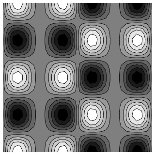
Figure 1: Contour plot of the potential in the small $\bar{f}/\overline{M}^{2}$ limit.

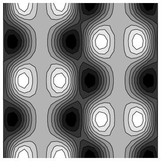
Figure 2: Contour plot of the potential for $\bar{f}/\overline{M}^{2}=0.5$.

Another interesting feature is the row of the minima in the case with finite $\bar{f}/\overline{M}^{2}$ in FIG. 2. Some topological configurations which connect the minima along the valley can be expected. Further study on the solitonic objects in the model should be done.

VI conclusion and discussion

In conclusion, we have shown that the one-loop finite potential for $N-2$ scalars is obtained from $N$ quantum fields. Though the fact may have been already known, we have explicitly found the $N-2$ degrees of freedom in the parameterization of the mass spectrum of quantum fields. To this end, we have utilized the expansion in terms of the modified Bessel functions.

The location of the potential extrema is not so sensitive to the two scales in the model. At the potential minimum, the mass eigenvalues of $N$ quantum fields are expected to be almost degenerate except for one. Therefore our model may provide us with a mechanism for spontaneous mass splitting of several fields.

The application to the particle-theory model is expected. We must make effort to clarify what symmetry enforces the mass matrix of $N$ fields and the (probably gauged) kinetic term of $N-2$ scalars to be the appropriate forms, and how symmetry breaking is triggered by the expectation value of scalars when gauge symmetry is incorporated. For this purpose, we have to take also diverse type of fields and their quantum effects into account. In this paper, we have only treated the scalar quantum field. We should consider the one-loop effect of fermions and gauge bosons for more natural particle theory. On the other hand, the higher-loop effects should be studied when interactions are introduced. We will perform more analyses of the effective potential for general models.

We can also cancel the scalar-independent divergent terms such as (13) and (14) by using fermionic quantum fields as well as bosonic fields without supersymmetry. This possiblity may shed light on new aspects of the cosmological constant problem and inflation mechanism.

In any case, the cosmological implications of the model will be revealed after analyzing more realistic models. Nevertheless we anticipate that the light scalar degrees of freedom becomes a candidate of dark matter or quintessence. Moreover, it may be interesting to study the finite temperature effect on the potential in the hot early universe.

References

(1) Y. Hosotani,
Phys. Lett. B126 (1983) 309.
D. J. Toms,
Phys. Lett. B126 (1983) 445.
(2) I. Antoniadis, K. Benakli and M. Quirós,
New J. Phys. 3 (2001) 20.
(3) D. M. Ghilencea, H. P. Nilles and S. Stieberger,
New J. Phys. 4 (2002) 15.
(4) N. Arkani-Hamed, A. G. Cohen and H. Georgi,
Phys. Rev. Lett. 86 (2001) 4757;
Phys. Lett. B513 (2001) 232.
C. T. Hill, S. Pokorski and J. Wang,
Phys. Rev. D64 (2001) 105005.
In early days, similar investigation has been done:
M. B. Halpern and W. Siegel,
Phys. Rev. D11 (1975) 2967.
(5) C. T. Hill and A. K. Leibovich,
Phys. Rev. D66 (2002) 016006,
hep-ph/0205057;
Phys. Rev. D66 (2002) 075010,
hep-ph/0205237.
(6) N. Kan, K. Sakamoto and K. Shiraishi,
The European Physical Journal C28 (2003) 425,
hep-th/0209096.
(7) K. Shiraishi, K. Sakamoto and N. Kan,
J. Phys. G: Nucl. Part. Phys. 29 (2003) 595, hep-ph/0209126.
(8) N. Kan and K. Shiraishi, “Multi-graviton theory, a
latticized dimension and the cosmological constant”, gr-qc/0212113.
(9) I. S. Gradstein and I. M. Ryshik,
Tables of integrals, sums, series and products,
Academic Press, New York (1980).
M. Abramowitz and I. Stegun (eds.),
Handbook of Mathematical Functions,
Dover, New York (1972).
(10) K. Lane,
Phys. Rev. D65 (2002) 115001.
(11) J. I. Kapusta,
Finite-temperature field theory, Cambridge University Press, 1989.
M. Le Bellac,
Thermal Field Theory, Cambridge University Press, 1996.