Lepton Electric Dipole Moments, Supersymmetric Seesaw and Leptogenesis Phase

Abstract

We calculate the lepton electric dipole moments in a class of supersymmetric seesaw models and explore the possibility that they may provide a way to probe some of the CP violating phases responsible for the origin of matter via leptogenesis. We show that in models where the right handed neutrino masses, $M_{R}$ arise from the breaking of local B-L by a Higgs field with B-L=2, some of the leptogenesis phases can lead to enhancement of the lepton dipole moments compared to the prediction of models where $M_{R}$ is either directly put in by hand or is a consequence of a higher dimensional operator.

I Introduction

A presently popular way to understand the origin of matter-anti-matter asymmetry in the universe is to start with a mechanism to generate lepton asymmetry in the early Universe using the CP violating effects in the decay of a heavy right handed Majorana neutrinosfy and let the sphaleron interactionskrs above the electroweak phase transtion temperature convert them to a baryon asymmetry. This is possible since the sphaleron interactions which violate B+L symmetry are in thermal equilibriumkrs above the eletcroweak phase transition temperature. The right handed neutrino decay is of course not the only way to generate the pre-electroweak lepton asymmetry. Several other ways have been discovered for the purpose (e.g. see references sm ; others ). We will however focus in this paper on the decay of heavy right handed neutrinos since they also provide a simple way to understand small neutrino masses via the seesaw mechanismseesaw . In particular, the existing experimental information on neutrino oscillations via the seesaw mechanism effects the nature of the right handed neutrino mass pattern. which in turn effects the magnitude of the baryon asymmetry. It is quite interesting that detailed analyses that use the exisitng neutrino data do indeed give the right magnitude for baryon asymmetry as well as important insight into the pattern of right handed neutrino massesbuch .

As noted in the original pioneering work of Sakharov, CP violation is an essential ingredient in the generation of any particle-anti-particle asymmetry. In the present case, the CP violating decays of the right handed neutrinos arise from the phases in right handed neutrino couplings and we will call them leptogenesis phases. It is clearly important to seek low energy manifestations of the leptogenesis phase for several reasons: first, this will improve our understanding of the right handed neutrino mass matrix which plays a crucial role in the neutrino mass physics at low energies; secondly, it may shed light on the origin of the seesaw mechanism, which will then provide a useful window into physics beyond the standard model. Moreover, since the seesaw formula provides some connection between the low and high scale phases in the theory, understanding leptogenesis phases may be a guide to the CP violating effects in neutrino oscillations, with its many experimental ramifications.

There have been a great deal of discussion of this issue in literature davidson . Specific models where the neutrino mass phase and leptogenesis phases are directly related have also been discussed in several papersendoh providing one way to probe the latter. However in all previous discussions of this issue, the masses of the right handed neutrinos $M_{R}$ are either put in by hand or are assumed to arise from nonrenormalizable operators. It is however well known that in models that contain Higgs bosons $\Delta$ with B-L=2, $M_{R}$ arises from a renormalizable coupling $f\nu^{c}\nu^{c}\Delta$. Examples of such theories are left-right symmetric models with triplet Higgs fields or SO(10) models with 126 dimensional Higgs fields, $SU(5)_{L}\times SU(5)_{R}$ models with Higgs fields in $(1,15)\oplus(15,1)$ representation. In such theories, there are new renormalization group running effects between the GUT (or Planck) scale and the seesaw scale. We showed in a previous paperbabu that the presence of these renormalizable couplings can lead to quantitatively different effects in seesaw induced lepton flavor violation. In particular, the ratio $B(\mu\rightarrow e+\gamma)/B(\tau\rightarrow\mu+\gamma)$ depends on the SUSY breaking parameters in very different ways in different theories.

In this paper, we calculate the electric dipole moments (edm) in the class of supersymmetric seesaw models with the $f$ coupling and discuss how it helps in probing the leptogenesis phase.

Since we are working within supersymmetric seesaw models, (i) we need to make assumptions about the nature of supersymmetry breaking and (ii) the embedding of MSSM into new physics at the seesaw scale.

As for the first point, in common with many discussions in the literature, we will assume that the TeV scale theory is the minimal supersymmetric standard model, which solves the gauge hierarchy problem plus the additional feature that the neutrinos have Majorana masses arising from the seesaw mechanism. As far as SUSY breaking is concerned, we will work within the context of minimal MSUGRA modelsmsugra and assume that around the GUT or the Planck scale, all soft SUSY breaking scalar masses are universal as are the gaugino masses and the A-terms are proportional to the Yukawa couplings. Furthermore we will assume that there are no overall phase in the $A$ terms, which is guaranteed if for example, MSSM is part of a left-right symmetric SUSY model near the GUT scalerasin . The resulting theory is a very economical one with only five parameters characterizing the complete susy breaking sector of MSSM and is therefore quite predictive. More importantly, the restrictive nature of this assumption means that at low energies, we are only tracking the effect of the phases in the right handed neutrino couplings responsible for leptogenesis and no other phase unrelated to neutrino physics is present. Once we give up these assumptions, new phases could come in and confuse the issue.

As far as the high theory theory is concerned, to implement our premise of having seesaw mechanism arise out of a B-L = 2 Higgs field, we will consider the high scale theory to be $SU(2)_{L}\times U(1)_{I_{3R}}\times U(1)_{B-L}$ based with a standard model singlet $\Delta$ with B-L =2 breaking the B-L gauge symmetry and also giving the seesaw mechanism. This model can arise as an effective theory from left-right or SO(10) theories. This extended model leaves the low energy predictions of MSSM uneffected.

The weak scale values of the supersymmetry breaking parameters can then be derived by the renormalization group extrapolations using the standard techniques. Since it is the dimension four terms in the Lagrangian which are largely responsible for the running, how the right handed neutrino masses are generated in the Lagrangian does make difference to low energy phenomenology. We discuss the impact of this extra running effect on the lepton dipole moment observable which depends on the leptogenesis phases.

The main result of our investigation is that if the right handed neutrino mass in the seesaw mechanism arises from the vev of a B-L=2 Higgs field, it has the effect of enhancing the lepton electric dipole moments over models where the right handed neutrino mass is put in by hand. We give two examples to illustrate this point: one where the neutrino mixings arise purely from Dirac Yukawa coupling of the right handed neutrinos and a second one where it arises from their Majorana coupling $f$. We also discuss the case of a $3\times 2$ seesaw models. In all the cases, a B-L=2 Higgs field is responsible for righthanded neutrino masses.

We present the results of our calculation for electron amd muon edms for the above models making sure that we stay in the range of parameters which fit all neutrino data and generate the right amount of lepton asymmetry. We find that leptogenesis phase can lead to enhanced edms for leptons in the presence of the $f$ couplings than in their absence (i.e. where the RH neutrino has a bare mass term.), although the effects are still small. Most optimistic values for electron edms in our models are between $10^{-30}$ to $10^{-31}$ ecm and for muon edm between $10^{-27}$ to $10^{-28}$ ecm. It is encouraging that there are ideas and plans for drastic improvement in the search for the lepton edms in the futurelamo ; seme ; miller . For instance, search for electrons edm upto the level of $10^{-31}$ ecmlamo and muon edm to $10^{-26}$ ecm have been contemplatedseme .

Although the values predicted by our analysis are small, high precision searches for lepton edms to the contemplated level can still teach us something useful. For instance, if the edms discovered are above our predictions, it will mean one of several things: either there is gross departures from the assumed forms for supersymmetry breaking terms or if independent experiments such as at LHC or Tevatron have confirmed the SUSY breaking assumptions (universality and proportionality), we would have to conclude that baryogenesis does not originate via leptogenesis. Either of these conclusions would be very important in our search for physics beyond the standard model.

We have organized this paper as follows: in sec. 2, we present a generic model based on the gauge group $SU(2)_{L}\times U(1)_{I_{3R}}\times U(1)_{B-L}$ to discuss the general calculational framework and the basic idea of our work; in sec 3, we discuss the renormalization group effects of the neutrino sector on the supersymmetry parameters. in sec.4, we present a qualitative explanation of how the enhancement of edm can arise in our approach; in sec. 5, we briefly discuss the calculation of baryogenesis; in sec. 6 we discuss the first neutrino mass model, give the neutrino mass fits, calculation of lepton asymmetry and present the results for lepton edms; in sec. 7 and 8, we repeat the same discussion for two other models; in sec. 9, we summarize our results and present the conclusions.

II A generic model and the calculational framework

To proceed with our discussion, let us write the superpotential for our model, which must be invariant under the gauge group $SU(2)_{L}\times U(1)_{I_{3R}}\times U(1)_{B-L}$:

$$W~{}=~{}e^{cT}{\bf Y_{\ell}}LH_{d}+{\nu^{c}}^{T}{\bf Y_{\nu}}LH_{u}+{\bf\frac{f}{2}\Delta}{\nu^{c}}^{T}\nu^{c}+S(\bar{\Delta}\Delta+\lambda H_{u}H_{d}+S^{2}-v^{2}_{R})$$ (1)

Here $L,e^{c},\nu^{c}$ are leptonic superfields; $H_{u,d},\Delta,\bar{\Delta}$ are the Higgs fields. We do not display the quark part of the superpotential but it is same as in the MSSM.

The first point to notice is that it is a very simple extension of the MSSM superpotential, that leads to a vacuum with ${\bf<\Delta>}=<\bar{\Delta}>=v_{R}$. This leads to the RH neutrino mass matrix $M_{R}~{}=~{}fv_{R}$ and clearly it arises from a renormalizable term in the Lagrangian.

This superpotential has also another advantage that it solves the $\mu$ problembabu1 i.e. it predicts that $\mu\simeq m_{3/2}$, where $m_{3/2}$ is the superpartner mass, which is of order of a TeV. To see this, notice that this potential has an R-symmetry under which $W\rightarrow-W$; (the fields transform as $(H_{u},e^{c},d^{c})\rightarrow i(H_{u},e^{c},d^{c})$; $(H_{d},\nu^{c},u^{c})\rightarrow-i(H_{d},\nu^{c},u^{c})$; $S\rightarrow-S$ and all other fields remain unchanged under R-symmetry). The vanishing of the F-terms then imply that $<S>=0$ and $<S>$ arises from supersymmetry breaking terms. As a result $\mu\simeq<S>\sim m_{3/2}$.

The seesaw formula (type I) can be written as:

$${\cal M}_{\nu}~{}=~{}-{\bf Y^{T}_{\nu}f^{-1}Y_{\nu}}\frac{v^{2}_{wk}tan^{2}\beta}{v_{R}}$$ (2)

We can choose a basis where the coupling matrix $f$ is diagonal as is the charged lepton Yukawa coupling matrix $Y_{\ell}$. The neutrino Dirac coupling matrix $Y_{\nu}$ is then a $3\times 3$ complex matrix whose diagonal elements can be made real by suitable redefinition of the phases of the $\ell_{i}$ and $e^{c}_{i}$ fields. This leaves us with nine real parameters in the $Y_{\nu}$ matrix and six phases. We rewrite the $Y_{\nu}$ matrix as follows:

$$Y_{\nu}~{}=~{}V^{*}Y^{d}_{\nu}W^{\dagger}$$ (3)

where $V~{}=~{}P_{1}\tilde{V}P_{2}$ with $P_{i}~{}=~{}diag(e^{i\phi_{i1}},e^{i\phi_{i2},1}$ and $\tilde{V}$ and $W$ are CKM type matrices with only one phase in each. Thus all six phases are accounted for.

To see which of the phases are responsible for lepton asymmetry, let us write down the formula for lepton asymmetry, $n_{\ell}$buch1 :

$$n_{\ell}\propto\sum_{j}Im[Y_{\nu}Y^{\dagger}_{\nu}]^{2}_{1j}F(\frac{M_{1}}{M_{j}})$$ (4)

where symbol 1 in the above equation denotes the lightest right handed neutrino eigenstate. Note that using Eq.3, one can conclude that only the phase in $\tilde{V}$ and those in $P_{1}$ contribute to lepton asymmetry. The phases in $P_{2}$ completely drop out. Our goal will therefore be to see how we can measure the phases in $P_{1}$ and $\tilde{V}$ by low energy experiments.

Secondly, we find two results for the three generation case that we state below.

II.1 Independence of light neutrino mixings and leptogenesis phases

The first point is that the lepton asymmetry parameter $n_{\ell}$ is independent of the PMNS mixing angles. To show this first note that

$${\cal M}_{\nu}~{}=~{}U^{*}{\cal M}^{d}_{\nu}U^{\dagger}~{}=~{}~{}-{\bf Y^{T}_{\nu}f^{-1}Y_{\nu}}m_{0}$$ (5)

where $m_{0}~{}=~{}\frac{v^{2}_{wk}tan^{2}\beta}{v_{R}}$ and $U$ is the PMNS mixing matrix. We can now invert the seesaw relation to conclude that

$$Y_{\nu}~{}=~{}if^{1/2}O({\cal M}^{d}_{\nu})^{1/2}U^{\dagger}$$ (6)

where $O$ is a complex matrix with the property that $OO^{T}=1$casas . The set of matrices $O$ in fact form a group analogous to the complex extension of the Lorentz group. Using Eq.6 in Eq.4, we see that lepton asymmetry $n_{\ell}$ is independent of the PMNS mixing angles in $U$rebelo . This result is important because what this means is that if there are three right handed neutrinos, low energy experiments such as neutrino oscillations and neutrinoless double beta decay give us no information about the leptogenesis phase.

II.2 Vanishing of lepton asymmetry for degenerate neutrino masses

To see this, we rewrite the formula for $n_{\ell}$ in a slightly different way. Using the seesaw formula in Eq.2 and assuming that there is a mass hierarchy among the right handed neutrinos, we can writebuch2

$$n_{\ell}\propto Im[Y_{\nu}{\cal M}^{\dagger}_{\nu}Y^{T}]_{11}$$ (7)

Using this and Eq.6, we can write

$$n_{\ell}\propto Im[f^{1/2}O({\cal M}^{d}_{\nu})^{2}O^{T}f^{1/2}$$ (8)

From this we can conclude that when the neutrino masses are degenerate i.e. ${\cal M}^{d}_{\nu}=m{\bf I}$, then $n_{\ell}=0$ since $f_{11}$ is real. This result, to the best of our knowledge does not exist in literature. A similar result for the manifestly CP violating observable $P_{\nu_{e}-\bar{\nu}_{e}}-P_{\bar{\nu}_{e}-\nu_{e}}$ was noticed in Ref.andre , where it was pointed out that it vanishes for degenerate neutrinos.

An implication of this result is that if neutrinoless double beta decay results imply $m\geq 0.1$ eV(see e.g. klap ), then the lepton asymmetry from RH neutrino decay will be suppressed by an extra factor of 100 and we might then have to look for extra enhancements or completely different way of obtaining the baryon asymmetry of the universe.

III RGE’s and low energy effects of leptogenesis phases

Let us now proceed to the main part of our discussion, which involves the supersymmetry breaking superpartner proiperties at low energies.

It is clear that one simple way to measure high scale parameters of a theory is to look for low energy observables that owe their origin or magnitude to the renormalization group evolution (RGE) from the high scale to the low scale (i.e. without RGE effects, the low energy theory will predict the observable to be very tiny.) In our case such observables are lepton flavor violating transitions as well as lepton electric dipole moments (edms). In the absence of the RGE effects, we expect $B(\mu\rightarrow e+\gamma)$ to be proportional to $\frac{m^{4}_{\nu}}{m^{4}_{W}}\sim 10^{-48}$ As far as the edm of leptons go, in the low energy theory without any other effects i.e. standard model with a Majorana mass for the neutrino, we would expect $d_{e}\simeq\frac{G_{F}m_{e}}{16\pi^{2}}\frac{m^{2}_{\nu}}{m^{2}_{W}}$ to be of order $10^{-48}$ ecm.

In supersymmetric models, the presence of superpartners introduce new contributions to both LFV as well as edm observables at the one loop level, where virtual superpartners flow inside the loop. The resulting LFV and edm effects are therefore not only enhanced but they are also sensitive to the nature of SUSY breaking terms. In this paper we will assume a very restrictive form for the SUSY breaking terms which defines the so called mSUGRA models. According to this assumption, the scalar masses and all gaugino masses are universal at the GUT or the Planck scale; the $A$ terms are proportional to the Yukawa couplings. These assumptions are motivated in several SUSY breaking scenarios; they not only reduce the number of parameters in the theory but may be necessary for understanding the observed suppression of flavor changing effects in both quark and lepton sectors. Furthermore, we will assume that the overall phase in the $A$ term is zero. This can happen for example, if the theory is part of SUSY left-right model at the GUT scalerasin . This is necessary in order to resolve the so-called SUSY CP problem.

The proportionality assumption coupled with the assumtion of no overall phase in the $A$ term guarantees that all the CP violating phases in the lepton sector sector are in the $Y_{\nu}$ and therefore any CP violating low energy effect after renormalization group evolution is only sensitive to the phases that are manifested in the leptogenesis as well as the neutrino oscillations via the seesaw mechanism.

As mentioned, we need to extrapolate the SUSY breaking parameters from the GUT or Planck scale down to the seesaw scale where we will perform the calculation of the electric dipole moments of the electron and the muon. This extrapolation will always involve the couplings $Y_{\nu}$ and the diagonal coupling matrix $Y_{\ell}$. Extrapolation below the seesaw scale only involves the $Y_{\ell}$ which is mostly diagonal to leading order and does not effect any of our results. We will keep only one loop effects. The relevant renormalization group equations are:

$$\frac{dY_{\nu}}{dt}~{}=~{}\frac{Y_{\nu}}{16\pi^{2}}[Tr(3Y_{u}Y^{\dagger}_{u}+Y_{\nu}Y^{\dagger}_{\nu})+3Y^{\dagger}_{\nu}Y_{\nu}+Y^{\dagger}_{\ell}Y_{\ell}-3g^{2}_{2}-g^{2}_{R}-3/2g^{2}_{B-L}]+\frac{1}{16\pi^{2}}ff^{\dagger}Y_{\nu}$$ (9)

$$\frac{dm^{2}_{L}}{dt}~{}=~{}\frac{1}{16\pi^{2}}[(m^{2}_{L}+2m^{2}_{H_{d}})Y^{\dagger}_{\ell}Y_{\ell}+(m^{2}_{L}+2H^{2}_{u})Y^{\dagger}_{\nu}Y_{\nu}+2Y^{\dagger}_{\ell}m^{2}_{e^{c}}Y_{\ell}+Y^{\dagger}_{\ell}Y_{\ell}m^{2}_{L}$$ (10)

$$+2Y^{\dagger}_{\nu}m^{2}_{\nu^{c}}Y_{\nu}+Y^{\dagger}_{\nu}Y_{\nu}m^{2}_{L}+2A^{\dagger}_{\ell}A_{\ell}+2A^{\dagger}_{\nu}A_{\nu}-6g^{2}_{2}M_{2}^{2}-3g^{2}_{B-L}M_{B-L}^{2}]$$

Let us also write down the renormalization group equations for the $A$ parameters- specifically the $A_{\ell}$.

$$\frac{dA_{\ell}}{dt} = \frac{1}{16\pi^{2}}[A_{\ell}[Tr(3Y^{\dagger}_{d}Y_{d}+Y^{\dagger}_{\ell}Y_{\ell})+5Y^{\dagger}_{\ell}Y_{\ell}+Y^{\dagger}_{\nu}Y_{\nu}$$

$$- 3g^{2}_{2}-g^{2}_{R}-3/2g^{2}_{B-L}]+Y_{\ell}[Tr(6A_{d}Y^{\dagger}_{d}+2A_{\ell}Y^{\dagger}_{\ell})$$

$$+ 4Y^{\dagger}_{\ell}A_{\ell}+2Y^{\dagger}_{\nu}A_{\nu}+6g^{2}_{2}M_{2}+2g^{2}_{R}M_{R}+3g^{2}_{B-L}M_{B-L}]]$$

$$\frac{dA_{\nu}}{dt} = \frac{1}{16\pi^{2}}[A_{\nu}[Tr(3Y^{\dagger}_{u}Y_{u}+Y^{\dagger}_{\nu}Y_{\nu})+5Y^{\dagger}_{\nu}Y_{\nu}+Y^{\dagger}_{\ell}Y_{\ell}$$

$$+ -3g^{2}_{2}-g^{2}_{R}-3/2g^{2}_{B-L}+4ff^{\dagger}A_{\nu}]+Y_{\nu}[Tr(6A_{u}Y^{\dagger}_{u}+2A_{\nu}Y^{\dagger}_{\nu})$$

$$+ 4Y^{\dagger}_{\nu}A_{\nu}+2Y^{\dagger}_{\ell}A_{\ell}+6g^{2}_{2}M_{2}+2g^{2}_{R}M_{R}+3g^{2}_{B-L}M_{B-L}]+8A_{f}f^{\dagger}Y_{\nu}]$$

While in presenting actual results, we numerically integrate these RGEs to obtain their contribution to physical observables such as lepton edms, it is instructive to give some approximate analytic expressions for the different results to get feeling for our final predictions. We do this in the following section.

IV Estimates of the electron and muon edms and connections to leptogenesis phase

To see the new effects from the $f$ couplings in a qualitative manner, we note that the dominant supersymmetric contributions to the lepton dipole moments come from the one loop diagram involving the bino. A rough estimate of this is

$$d^{e}_{\ell_{i}}\simeq\frac{g^{2}_{1}}{8\pi^{2}M^{4}_{\tilde{\ell},0}}Im(A_{\ell}M^{2}_{\ell})$$ (13)

If there is an overall phase in $A_{\ell}$, then one can easily estimate $d^{e}_{e}\simeq 10^{-23}sin\delta$ ecm. To be consistent with present limits i.e. $\leq 1.7\times 10^{-27}$ ecm, one must have phase $\delta\leq 10^{-3}$. This is the so called SUSY phase problem. We assume that in the theory the SUSY CP problem has been solved, (e.g. by embedding the MSSM into a SUSY LR model as mentioned) so that we can set $\delta=0$. In this limit, in the absence of the RGE effects, since $M^{2}$ is real, in this limit, all edms vanish. If this term dominated the contribution to the lepton dipole moments, then since the $A$ term id proportional to charged lepton masses, we would have the scaling law $d^{e}_{\mu}/d^{e}_{e}=m_{\mu}/m_{e}$. In any theory where this law holds, the present upper limit on electron edm of $\leq 4.3\times 10^{-27}$ ecm would imply that $d^{e}_{\mu}\leq 8.6\times 10^{-15}$ ecm. Also this scaling law is a signature of the simplicity of the underlying theory. In the supersymmetric context, there exist exceptions to this scaling lawbabu2 .

After RGE effects are taken into account, lepton edms receive contributions from $Y^{\dagger}_{\nu}Y_{\nu}$ which is not a diagonal matrix as well as $f^{\dagger}f$ and $Y^{2}_{\ell}$ which are diagonal matrices at the GUT scale. The $M^{2}$ and $A_{\ell}$ at the seesaw scale are polynomials in these matrices and in order to get a nonvanishing contribution to $d^{e}_{\ell}$, we must look for imaqginary diagonal elements in the product $A_{\ell}M^{2}_{\tilde{\ell}}$, which will involve products of $Y^{\dagger}_{\nu}Y_{\nu}$, $f^{\dagger}f$ and $Y^{2}_{\ell}$.

The leading order term in $A_{\ell}M^{2}_{\tilde{\ell}}$ in the absence of the $f$ couplings (i.e. a bare mass term for $\nu_{R}$), which has a complex $11$ entry is of the form

$$d^{e}_{\ell}\propto Im[m_{0}Y_{\ell}Y^{\dagger}_{\nu}Y_{\nu}Y^{2}_{\ell}(Y^{\dagger}_{\nu}Y_{\nu})^{2}].$$ (14)

From Eq. (3), it is easy to see that $Y^{\dagger}_{\nu}Y_{\nu}$ is independent of the matrix $V$ that is responsible for leptogenesis. One might conclude from this that simple RGE extrapolations like this term will never enable us to probe the matrix $V$. However, as has been argued insacha , since $Y^{\dagger}_{\nu}Y_{\nu}$ is sensitive to the unitary matrix $W$ in Eq. (3). So in principle, one can get $W$ from the experimental information about supersymmetry breaking sector. Then, if one is given the right handed neutrino mass spectrum and the form of $Y_{\nu}$, one can get all the matrix elements of $V$ using the relation

$$V^{T}fV~{}=~{}-(Y^{d}_{\nu})^{-1}W^{T}U^{*}{\cal M}^{d}_{\nu}U^{\dagger}W(Y^{d}_{\nu})^{-1}$$ (15)

and hence the baryogenesis phases. This would require knowledge of all the matrix elements of slepton mass matrix. While this is possible in principle, one would like a more “experimentally feasible” way to probe the phases in $V$. This is what we pursue here.

There are two ways in which the RGE extrapolation can still leave traces of the matrix $V$. One way discussed in ellis is the following. In the case where the right handed neutrino masses are hierarchical, the simple RGE expression in the above paragraph gets modified by threshold effects as follows: the simple expression in Eq.14 remains valid above the highest right handed neutrino mass, $M_{3}$; once we go below this i.e. for $M_{2}\leq\mu\leq M_{3}$, only the second and the lightest RH neutrinos contribute. This means that in the matrix $Y_{\nu}$, only $Y_{\nu,2i}$ and $Y_{\nu,1i}$ contribute and below $M_{2}$ only $Y_{\nu,1i}$ entries contribute. Therefore traces of the matrix $V$ remain in the low energy expressions. To get a large effect, a significant gap between the $M_{3}$ and $M_{1}$ is required.

Another way that $V$ can be visible is the presence of the $f$ terms, which give the leading contribution to edm to be $Y^{\dagger}_{\nu}Y_{\nu}Y^{\dagger}_{\nu}f^{\dagger}fY_{\nu}$ instead of what is given in 14. Thus in this case, there is a higher order effect even in the absence of threshold effects.

Note further that each time a term of the form $Y^{\dagger}_{\nu}Y_{\nu}$ or $f^{\dagger}f$ appears, there is a loop suppression factor $\epsilon_{loop}\simeq\frac{1}{16\pi^{2}}\ell n\left(\frac{M_{U}}{M_{R}}\right)\simeq 0.06-0.1$. Taking this into account we see that the second contribution (i.e. one in the presence of the $f$ couplings) is enhance by the inverse of one loop factor compared to the first one. Also, there is an additional effect coming from the gap between the $M_{U}$ or $M_{P\ell}$ and $M_{3}$. Therefore barring unexpected cancellations, we expect the edm contribution in the presence of $f$ contributions to be bigger. In our numerical integrations to present the final numbers for edms, we keep the threshold effects.

V Overview of Baryogenesis estimate

As already mentioned earlier, we use the mSUGRA framework to calculate the electric dipole moments of the muon and the electron. The value of the universal scalar mass $m_{0}$, universal gaugino mass $m_{1/2}$, universal trilinear term $A_{0}$, $\tan\beta$ and the sign of $mu$ as free parameters determine our final result. We also assume that there is no phase associated with the SUSY breaking. The Yukawa and/or the Majorana couplings are responsible for CP violation in these models.

The mSUGRA parameter space is constrained by the experimental lower limit on $m_{h}$ and the measurements of $b\rightarrow s\gamma$ and the recent results on dark matter relic densitywmap . For low $\tan\beta$, the parameter space has lower bound on $m_{1/2}$ from the light Higgs mass bound of $m_{h}\geq 114$ GeV. For larger $\tan\beta$ the lower bound on $m_{1/2}$ is produced by the CLEO constraint on the BR($b\rightarrow s\gamma$). The recent WMAP results have led to stronger constraints on dark matter density which in turn reduces the allowed parameter space of mSUGRA mostly to the co-annihilation region for $m_{0},\,m_{1/2}\leq 1000$ GeV.

We calculate the baryon to photon ratio $\eta_{B}$ in three different models for neutrino masses. The SUSY breaking parameters do not play a role in this discussion. The lepton asymmetry is produced from the out of equilibrium decays of right handed neutrinos and this gets converted into baryon asymmetry through the sphaleron processes. The formula for $\eta_{B}$ is:

$$\eta_{B}={n_{B}\over{n_{\gamma}}}={ag_{s}^{0}}\sum{{\kappa_{i}\epsilon_{i}}\over{g^{*}}}$$ (16)

where $a$ relates the B-L asymmetry to baryon asymmetry and ${ag_{s}^{0}\over{g^{*}}}\sim 5\times 10^{-3}$. $\kappa$ is the washout factor buch1 and $\epsilon_{i}={1\over{8\pi}}\sum_{k\neq i}(f({{|M_{k}|^{2}}\over{|M_{i}|^{2}}})+g({{|M_{k}|^{2}}\over{|M_{i}|^{2}}})){{Im[(h^{{\dagger}}h)^{2}_{ik}]}\over{(h^{{\dagger}}h)_{ii}}}$buch1 with $f(x)=\sqrt{x}[ln({{1+x}\over{x}})]$ and $g(x)=2{\sqrt{x}\over{1-x}}$.

The recent experimental bound on $\eta_{B}$ iswm :

$$\eta_{B}=(6.5\pm^{0.4}_{0.3})\times 10^{-10}$$ (17)

In the following sections, we will use these expressions to evaluate the baryon asymmetry, which along with present neutrino oscillation results will then give us a range of parameters in the seesaw formula. We will use these parameters to calculate the edms of the electron and the muon using the allowed range of SUSY breaking parameters mentioned above.

We present three different cases. In at least one case, the effects are big enough that they are within reach of contemplated experiments for the elctronlamo . Planned searches for the muon edmmiller will also throw important light on this issue.

VI First model for neutrino masses and its predictions for lepton edms

In this section, we consider the first of three examples for neutrino masses and obtain the predictions for lepton edms in the presence of the $f$ terms. In this example, we take the $Y_{\nu}$ and $Y_{\ell}$ to be diagonal and assume that all neutrino mixings to arise from arbitrary complex $f$ couplingbabu . In the notation of sec. 2, this means that $W$ is a identity matrix. Clearly therefore, in the absence of the $f$ term contributions, edm becomes very tiny ($\leq 10^{-48}$ ecm. The $f$ couplings lead to an enhancement of the effects of leptogenesis phases in the lepton edms as we see below.

As for the $Y_{\nu}$, we consider two subcases: (a) in the first case we let the diagonal elements of $Y_{\nu}$ be free and (b) in this second case, we let them be proportional to the charged lepton masses.

In both cases, we can write the matrix elements of $f$ in terms of the diagonal elements of $Y_{\nu}$ i.e. $(c\epsilon^{3},\epsilon,1)y$ and the neutrino mass matrix. For this purpose, we take the light neutrino mass matrix to be:

$${\cal M}_{\nu}=m_{0}\left(\matrix{e\epsilon^{n}&h\epsilon^{m}&d\epsilon\cr h\epsilon^{m}&1+a\epsilon&1\cr d\epsilon&1&1+b\epsilon}\right)~{}.$$ (18)

Here $(a,~{}b,~{}d,~{}e,~{}h)$ are order one coefficients, $\Delta m^{2}_{atm}\simeq 4m_{0}^{2}$ and the exponents $(n,~{}m)$ in the (1,1) and (1,2) entries have to be at least 1, but can be larger. This matrix provides a good fit to all neutrino data. Using these, we get for $f$ matrix:

$$f={1\over d^{2}m_{0}}\left(\matrix{(a+b)c^{2}\epsilon^{5}&cd\epsilon^{3}&-cd\epsilon^{2}\cr cd\epsilon^{3}&-d^{2}\epsilon^{2}&dh\epsilon^{2}\cr-cd\epsilon^{2}&dh\epsilon^{2}&(e-h^{2})\epsilon^{2}}\right)~{}.$$ (19)

We now calculate the edms and $\eta_{B}$ in this model. For example, at $\tan\beta=30$:
we have ${f}$ at $2\times 10^{12}$ GeV

$${f} = \left(\matrix{-1.14\times 10^{-4}&-1.56\times 10^{-2}&0.293\cr-1.56\times 10^{-2}&0.379-0.353i&-0.21+0.55i\cr 0.293&-0.21+0.55i&0.058-0.091*i}\right)$$ (20)

We now assume that the Dirac neutrino mass is proportional to the charged lepton mass and are $0.0337,\,6.94,\,123.398$ GeV. Using these parameters, we find $\sin^{2}2\theta_{\odot}=0.8$, $\Delta m^{2}_{\odot}=5\times 10^{-5}$ eV² and $\sin^{2}2\theta_{A}=0.98$, $\Delta m^{2}_{A}=6\times 10^{-3}$ eV². In the calculation we decouple the neutrinos at the respective mass scales. The baryon to photon ratio is $\eta_{B}\sim 6\times 10^{-10}$. We will use these inputs to evaluate the lepton edms. Our results for edms are given in Fig 1 and 2.

In Fig.1 we plot the electric dipole moments of electron and the muon as functions of $A_{0}$ and $m_{1/2}$ and $m_{0}$ for $\tan\beta=10$. We do not show explicitly the values of $m_{0}$ since we choose their values in such a way so that the relic density constraint is satisfied in the only available stau-neutralino co-annihilation region for the parameter space. We apply the recent relic density constraint i.e. $0.094<\Omega h^{2}<0.129$ (2$\sigma$)wmap . Using this constraint, the maximum value of $m_{1/2}$ is found to be 800 GeV for $\tan\beta=10$. The magnitude $d_{\mu}$ can be as large as $10^{-29}$ ecm for $A_{0}=800GeV$, where as the $d_{e}$ can be as large as $10^{-34}$ ecm.

In Fig.2, we show the $d_{\mu}$ and the $d_{e}$ for the same model using $\tan\beta=30$. As expected the edms are larger in this case with $d_{\mu}$ as large as $4\times 10^{-28}$ ecm.

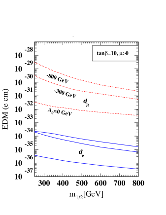
Figure 1: Electric dipole moments of electron $|d_{e}|$ (solid line) and muon $|d_{\mu}|$ (dotted line) for different values of $A_{0}$ for $\tan\beta=10$.

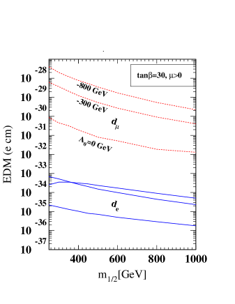
Figure 2: Electric dipole moments of electron $d_{e}$ (solid line) and muon $d_{\mu}$ (dotted line) for different values of $A_{0}$ for $\tan\beta=30$.

VII Model II for neutrino masses and predictions for lepton edm

In this case, we choose $Y_{\ell}$ and $f$ matrices to be diagonal and $f$ equal to $Diag(\epsilon^{6}_{f},\epsilon^{4}_{f},1)$ but keep a general form for $Y_{\nu}$ as follows:

$${Y}_{\nu}=\left(\matrix{0&h\epsilon^{3}&d\epsilon^{3}\cr h\epsilon^{3}&a\epsilon^{2}&b\epsilon^{2}\cr d\epsilon^{3}&b\epsilon^{2}&e^{i\psi}}\right)~{}.$$ (21)

For $\epsilon\simeq\epsilon_{f}\ll 1$ and $a,b\sim 1$ but complex, we get large solar and atmospheric neutrino mixings. We have done a detailed fit to the neutrino parameters keeping $a,b,h,d$ complex and have calculated the baryon asymmetry and the lepton edms. For example, at $\tan\beta=10$:
we have ${f}$ at $2.5\times 10^{15}$ GeV

$${f} = Diag[\left(\matrix{6.4\times 10^{-5}&1.6\times 10^{-3}&1}\right)]$$ (22)

The Dirac neutrino coupling is

$${Y_{\nu}} = \left(\matrix{0&1.67\times 10^{-2}-1.43\times 10^{-2}i&-2.31\times 10^{-2}-7.7\times 10^{-3}i\cr 1.67\times 10^{-3}-1.43\times 10^{-2}i&6.4\times 10^{-2}+1.1\times 10^{-1}i&8.3\times 10^{-2}-1.14\times 10^{-1}i\cr-2.31\times 10^{-2}-7.7\times 10^{-3}i&8.3\times 10^{-2}-1.14\times 10^{-1}i&-0.57i}\right)$$ (23)

Using these parameters, we find $\sin^{2}2\theta_{\odot}=0.83$, $\Delta m^{2}_{\odot}=5\times 10^{-5}$ eV² and $\sin^{2}2\theta_{A}=0.88$, $\Delta m^{2}_{A}=2\times 10^{-2}$ eV². The baryon to photon ratio is $\eta_{B}\sim 6\times 10^{-10}$.

In Fig.3 we plot the electric dipole moments of electron and the muon as functions of $A_{0}$ and $m_{1/2}$ and $m_{0}$ for $\tan\beta=10$. The relic density constraint is satisfied in the only available stau-neutralino co-annihilation region as before. The magnitude $d_{mu}$ can be as large as $10^{-28.5}$ ecm for $A_{0}=800GeV$, where as the $d_{e}$ can be as large as $10^{-32}$ ecm.

In Fig.4, we increase the scale where the universality and proportionality assumptions are made to $10^{18}$ GeV and study its effect on $d_{mu}$ as a function of $m_{1/2}$ for $A_{0}=300$ GeV. One needs to be careful about the size of the couplings at this new scale. The effects of the $f$ couplings in this new region increase the dipole moments. The top line shows the dipole moment for the increased scale and we conclude that the edm increases as the scale moves up.

Note that all these values are considerably above the values in the absence of the $f$ couplingsellis . Also note the violation of the mass scaling law for the dipole moments in the presence of the $f$ couplings.

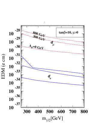
Figure 3: Electric dipole moments of electron $|d_{e}|$ (solid line) and muon $|d_{\mu}|$ (dotted line) for different values of $A_{0}$ for $\tan\beta=10$.

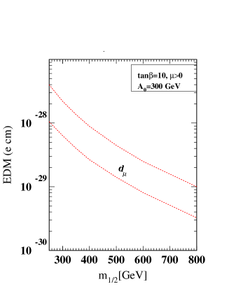
Figure 4: Electric dipole moments of muon $d_{\mu}$ for $M_{G}=2.3\times 10^{16}$ GeV and $10^{18}$ GeV

VIII The case of two $\nu_{R}$’s and the $3\times 2$ seesaw

In this section, we consider the predictions of a class of models with $3\times 2$ seesaw considered in various paperskuchi ; endoh ; king . First point to note is that the general results we discussed for the case of three right handed neutrinos in sec.2 do not apply to this case. In particular, as has been shown by Endoh et alendoh , the leptogenesis phase and the PMNS phases are directly related in this model unlike the three RH neutrino case.

To proceed with the investigation of this model, one can choose a basis such that $Y_{\ell}$ and $f$ are diagonal. The most general $3\times 2$ matrix $Y_{\nu}$ can now be parameterized as:

$$Y_{\nu}~{}=~{}V\left(\matrix{0&m_{2}&0\cr 0&0&m_{3}}\right)U$$ (24)

where $V~{}=~{}\left(\matrix{c&s\cr-s&c}\right)\left(\matrix{e^{i\gamma_{R}}&0\cr 0&e^{-i\gamma_{R}}}\right)$ and $U~{}=~{}O_{23}(\theta_{23})U_{13}(\theta_{13},\delta)O_{12}(\theta_{12})P_{L}$ where $P_{L}=\left(\matrix{e^{i\gamma_{L}}&0\cr 0&e^{-i\gamma_{L}}}\right)$.

In order to calculate the edms and $\eta_{B}$, we will work with the horizontal model of Ref.kuchi ; dm , which leads to a specific realization of the $3\times 2$ seesaw formula. The model is based on the gauge group $SU(3)_{c}\times SU(2)_{L}\times U(1)_{Y}\times SU(2)_{H}$ with fermion assignments given as follows:

Table I

$\Psi\equiv(L_{e},L_{\mu})$	(1,2,-1,2)
$L_{\tau}$	(1,2,-1,1)
$E^{c}\equiv(\mu^{c},-e^{c})$	(1,1,-2, 2)
$\tau^{c}$	(1,1,-2, 1)
$N^{c}\equiv(\nu^{c}_{\mu},-\nu^{c}_{e})$	(1,1,0,2)
$\nu^{c}_{\tau}$	(1,1,0,1)
$\chi_{H}\equiv\left(\begin{array}[]{cc}\chi_{1}&\chi_{2}\\ \end{array}\right)$	(1, 1, 0, 2)
$\bar{\chi}_{H}\equiv\left(\begin{array}[]{cc}-\bar{\chi}_{2}&\bar{\chi}_{1}\\ \end{array}\right)$	(1,1,0,2)
$H_{u}$	(1,2,+1,1)
$H_{d}$	(1,2,-1,1)
$\Delta_{H}$	(1,1,0,3)

Table caption: We display the quantum number of the matter and Higgs superfields of our model.

Here $L_{e,\mu,\tau}$ denote the left handed lepton doublet superfields. Other symbols are self explanatory. We arrange the Higgs potential in such a way that the $SU(2)_{H}$ symmetry is broken by $<\chi_{1}>=<\bar{\chi}_{2}>=v_{H1};<\chi_{2}>=<\bar{\chi}_{1}>=v_{H2}$ and $<\Delta_{H,3}>=v^{\prime}_{H}$, where $v_{H,i},v^{\prime}_{H}\gg v_{wk}$. The vevs for $\bar{\chi}$ are chosen so as to cancel the D-terms and leave supersymmetry unbroken below the scale of horizontal symmetry breaking.

The Yukawa superpotential for this model is given by:

$$W_{Y} = h_{0}(L_{e}H_{u}\nu^{c}_{e}+L_{\mu}H_{u}\nu^{c}_{\mu})+h_{1}L_{\tau}(\nu^{c}_{\mu}\chi_{2}+\nu^{c}_{e}\chi_{1})H_{u}/M-ifN^{cT}\tau_{2}{\bf\tau\cdot\Delta_{H}}N^{c}$$

$$\frac{h^{\prime}_{1}}{M}(L_{e}\chi_{2}-L_{\mu}\chi_{1})H_{d}\tau^{c}+\frac{h^{\prime}_{4}}{M}L_{\tau}H_{d}(\mu^{c}\chi_{2}+e^{c}\chi_{1})+{h^{\prime}_{3}}L_{\tau}H_{d}\tau^{c}+h^{\prime}_{2}(L_{e}e^{c}+L_{\mu}\mu^{c})H_{d}$$

The parameters in the above equation have been determined to fit neutrino mass data at low energiesdm . We use them in our calculation. We expect the predictions to be typical of most $3\times 2$ models. From dm , we see that at $\tan\beta=30$, the charged lepton mass matrix is given by (at the scale $10^{13}$ GeV):

$${\cal M}_{\ell} = \left(\matrix{7.5\times 10^{-3}&0&-1.135\cr 0&7.5\times 10^{-3}&0.247\cr 2.14\times 10^{-2}&0.0984&0.85}\right).$$ (26)

This determines all the Yukawa couplings responsible for charged lepton masses to be $h_{1}^{\prime}=1.135\times 10^{-1}$, $h_{2}^{\prime}=1.29\times 10^{-3}$, $h_{3}^{\prime}=1.466\times 10^{-1}$ and $h_{4}^{\prime}=9.8\times 10^{-3}$ with $\kappa_{2}=10$ and ${\kappa_{2}\over\kappa_{1}}=4.588$. We get the correct values of charged lepton masses at the weak scale from the above matrix. We use the MSSM RGEs between the horizontal scale and the weak scale. The $f$ is given at the horizontal scale:

$$f = \left(\matrix{5\times 10^{-3}&0.025+0.499i\cr 0.025+0.499i&2.5\times 10^{-3}}\right).$$ (27)

Using the same $\kappa$s as above, $h_{0}=9.2\times 10^{-2}$ and $h_{1}=-2.92\times 10^{-1}$, we find $\sin^{2}2\theta_{\odot}=0.87$, $\Delta m^{2}_{\odot}=7.5\times 10^{-5}$ eV², $\sin^{2}2\theta_{A}=0.88$, $\Delta m^{2}_{A}=2.48\times 10^{-3}$ eV² and $|U_{e3}|=0.11$ which are within the experimentally allowed regions. We find $\eta_{B}\sim 6\times 10^{-10}$.

In Fig.5 we plot the electric dipole moments of electron and the muon as functions of $m_{1/2}$ and $m_{0}$ for $\tan\beta=30$ and $A_{0}=300$ GeV. We again satisfy the relic dark matter density constraint. We find that unlike other models, both $d_{mu}$ and $d_{e}$ are of same order and as large as $10^{-31}$ ecm.

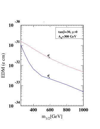
Figure 5: Electric dipole moments of electron $d_{e}$ (solid line) and muon $d_{\mu}$ (dotted line) for different values of $A_{0}$ for $\tan\beta=30$. The model parameters are described in the text.

To be completely phenomenologically consistent, we need to study the profile of lepton flavor violation for all these models. For model 1, this has been studied extensively in babu1 and the results are within the present bounds but quite testable as has been emphasized. Similarly, the branching ratio for $\mu\rightarrow e\gamma$ in model 3 can be found in ref.dm . We will therefore only calculate BR[$\mu\rightarrow e\gamma$] for model 2 for our choice of parameters and present them in fig.6 for different values of $m_{1/2}$ and $A_{0}$. We again demand the relic density constraint to be satisfied in this parameter space. We find that the most region of the parameter space is allowed by this branching ratio. The BR for $\tau\rightarrow\mu\gamma$ is $\sim 10^{-8}-10^{-14}$ in the same region parameter space.

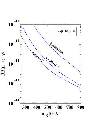
Figure 6: The branching ratio for $\mu\rightarrow e+\gamma$ for model 2.

IX Summary and conclusion

In summary, we have calculated the electric dipole moment of the electron and the muon in supersymmetric seesaw models where right handed neutrino masses arise from renormalizable coupling in the superpotential. Using this we have attempted to probe the CP violating phases in the right handed neutrino mass matrix responsible for leptogenesis. We consider the minimal gauge group which allows for this. We make the simple and widely used choice for the supersymmetry breaking parameters as in the mSUGRA models so that no new phases enter the discussion, other than the phases in the RH neutrino mass matrix which manifest at low energies and in leptogenesis. We find that due to the fact that the right handed neutrino masses arise via renormalizable couplings, the lepton edms get enhanced and in some models come within the range accessible to proposed experiments. For instance, we can have $d_{e}$ as large as $10^{-31}$ ecm. The largest values for muon edm we predict are at the level of $10^{-27.3}$ ecm. Also, the scaling law $d_{m}u/d_{e}~{}=~{}m_{\mu}/m_{e}$ does not hold in general. All the parameters of our model are chosen so that they are consistent with present neutrino data and the produce the required baryon asymmetry. The smallness of the edm values in most cases is due to the assumptions of complete universality of scalar masses in the MSSM and the proportionality of the $A$ terms to the Yukawa coupling. To the extent that collider experiments have the potential to confirm or rule out the mSUGRA models in the near future, these results can teach us important things about the origin of matter as well as about the origin of neutrino masses.

Clearly if the assumtions about SUSY breaking terms is relaxed, one can enhance the edm values further. One must then make sure that new phases not connected to leptogenesis are not responsible for the enhancement. In the minimal model there is no such confusion. This possibility is presently under consideration.

The work of R. N. M. is supported by the National Science Foundation Grant No. PHY-0099544 and that of B. D. by the Natural Sciences and Engineering Research Council of Canada. We like to thank K. S. Babu, S. Davidson and W. Buchmuller for discussions. One of us (R. N. M.) would like to thank G. Kane and the Michigan Center for Theoretical Physics for hospitality when the work was in its last stages and for the opportunity to present this work at the workshop on Baryogenesis prior to publication.

References

- (1) V. Kuzmin, V. Rubakov and M. Shaposnikov, Phys. Lett.
- (2) M. Fukugita and T. Yanagida, Phys. Lett. B174 45, (1986).
- (3) E. Akhmedov, V. Rubakov and A. Yu Smirnov, Phys. Rev. Lett. 81, 1359 (1998);
- (4) K. Dick, M. Lindner, M. Ratz and D. Wright, Phys. Rev. Lett 84, 4039 (2000); H. Murayama and T. Yanagida, Phys. Lett. B322, 349 (1994).
- (5) M. Gell-Mann, P. Ramond and R. Slansky, in Supergravity, eds. P. van Niewenhuizen and D.Z. Freedman (North Holland 1979); T. Yanagida, in Proceedings of Workshop on Unified Theory and Baryon number in the Universe, eds. O. Sawada and A. Sugamoto (KEK 1979); R. N. Mohapatra and G. Senjanović, Phys. Rev. Lett. 44, 912 (1980); S. L. Glashow, Cargese lectures, (1979).
- (6) M. Luty, Phys. Rev. D 45, 455 (1992); M. Flanz, E. A. Paschos and U. Sarkar, Phys. Lett. B345, 248 (1995); L. Covi, E. Roulet and F. Vissani, Phys. Lett. B 384, 169 (1996); A. Pilaftsis, hep-ph/9707235; W. Buchmuller and M. Plumacher, Phys. Lett. B 431, 354 (1998); A. S. Joshipura, E. A. Paschos and W. Rodejohann, JHEP 08, 029 (2001). W. Buchmuller, P. di Bari and M. Plumacher, hep-ph/0209301; E. Nezri and J. Orloff, JHEP, 0304, 020 (2003); E. Kh. Akhmedov, M. Frigerio and A. Yu Smirnov, hep-ph/0305322.
- (7) S. Davidson and A. Ibarra, Nucl. Phys. B 648, 345 (2003); J. Ellis, J. Hisano, M. Raidal and Y. Shimizu, Phys. Lett. B 526, 86 (2002); J. Ellis and M. Raidal,hep-ph/0206174; G. Branco, R. Gonzales-Felipe, F. R. Joaquim and M. N. rebelo, hep-ph/0202030; G. Branco, R. Gonzalez-Felipa, F. Joaquim, I. Masina, M. N. Rebelo and C. Savoy, hep-ph/0211001; S. F. King, hep-ph/0211228; D. Falcone and F. Tramontano, hep-ph/0011053; A. Broncano, M.B. Gavela, E. Jenkins, hep-ph/0307058; L. Velasco-Sevilla,hep-ph/0307071.
- (8) P. Frampton, S. L. Glashow and Yanagida, Phys. Lett. B 548, 119 (2002); T. Endoh, S. Kaneko, S. F. kang, T. Morozumi and M. Tanimoto, hep-ph/0209098.
- (9) K. S. Babu, B. Dutta and R. N. Mohapatra, Phys. Rev. D 67, 076006 (2003).
- (10) A. Chamsheddine, R. Arnowitt and P. Nath, N=1 Supergravity, World Scintific, Singapore (1984); R. Barbieri, S. Farrara and C. Savoy, Phys. Lett. B119, 343 (1982); L. Hall, J. Lykken and S. Weinberg, Phys. Rev.D27, 2359 (1983).
- (11) K. S. Babu, B. Dutta, R. N. Mohapatra, Phys.Rev. D61, 091701 (2000).
- (12) S. Lamoreaux, nucl-ex/0109014; F.J.M. Farley, K. Jungmann, J.P. Miller, W.M. Morse, Y.F. Orlov, Y.K. Semertzidis, A. Silenko, E.J. Stephenson, hep-ex/0307006; J. Aysto et al. hep-ph/0109217.
- (13) Y. Semertzidis et al. hep-ph/0012087.
- (14) J. Miller, Invited talk at the CIPANP 2003, May, 2003; W. Morse, Invited talk at the Nufact’03 workshop, New York, June (2003).
- (15) K. S. Babu, B. Dutta and R. N. Mohapatra, Phys. Rev. D 65, 016005 (2002) (hep-ph/0107089); R. Kitano and N. Okada, Prog. Theor. Phys. 106, 1239 (2001) (hep-ph/0107084).
- (16) L. Covi, E. Roulet and F. Vissani, Phys. Lett. B 384, 169 (1996); W. Buchmuller and M. Plumacher, Phys. Lett. B 431, 354 (1998); K. Hamaguchi, hep-ph/0212305; M. plumacher, Phys. Rept. 320, 329, (1999).
- (17) J. A. Casas and A. Ibarra, hep-ph/0103065.
- (18) M. Rebelo, Phys. Rev. D 67, 013008 (2003).
- (19) W. Buchmuller and S. Fredenhagen, Phys. Lett. B 483, 217 (2000).
- (20) A. de Gouvea, B. Kayser and R. N. Mohapatra, Phys. Rev. D 67, 053004 (2003) [arXiv:hep-ph/0211394].
- (21) H.V. Klapdor-Kleingrothaus et al., hep-ph/0201231; Nucl.Phys. Proc. Suppl. 100, 309 (2001).
- (22) K. S. Babu, B. Dutta and R. N. Mohapatra, Phys. Rev. Lett. 85, 5064 (2000).
- (23) S. Davidson and A. Ibarra, Ref.davidson .
- (24) J. Ellis et al, Ref.davidson hep-ph/0111324.
- (25) D.N. Spergel et.al. astro-ph/0302209; S. Hannestad, astro-ph/0303076.
- (26) C. L. Bennett et al, astro-ph/0302207; D. N. Spergel et al, astro-ph/0302209.
- (27) R. Kuchimanchi and R. N. Mohapatra, Phys. Rev. D 66, 051301 (2002); Phys. Lett. B 552, 198 (2003).
- (28) S. F. King, Nucl. Phys. B 576, 85 (2000); S. F. King and N. N. Singh, Nucl. Phys. B 596, 81 (2001); W. Grimus and L. Lavoura, Phys. Rev. D 62, 093012 (2000).
- (29) B. Dutta and R. Mohapatra, hep-ph/0305059.