REVTeX 4 Prediction of Neutron Elastic Form Factors Using GPDs from Proton Elastic Form Factors and Isospin Symmetry

Abstract

The elastic neutron form factors $G_{En}$ and $G_{Mn}$ are calculated in a GPD framework using GPDs obtained from fits to proton elastic form factors $G_{Ep}$ and $G_{Mp}$, and isospin symmetry, with no further changes in parameters. The results for $G_{En}$ are in good agreement with existing data, while those for $G_{Mn}$ are fair. The calculations predict the form factors for future measurements at higher $Q^{2}$.

In recent years, the development of generalized parton distributions (GPDs)  ji ; rad_gpd ; collins has opened the possibility of describing a great variety of exclusive reaction in the multi GeV range in terms of a common nucleon structure. The constraints imposed by the description of many types of reactions offers the possibility of modeling the longitudinal and transverse parton structure of nucleons.

Among the most direct consequences of the GPD formalism are the sum rules which relate the various GPDs to the hadronic form factors. Thus the proton elastic helicity conserving and helicity-flip form factors may be written, respectively, as :

$$F_{1p}(t)=\int^{1}_{-1}\sum_{q}e_{q}H_{p}^{q}(x,\xi,t)dx$$

$$F_{2p}(t)=\int^{1}_{-1}\sum_{q}e_{q}E_{p}^{q}(x,\xi,t)dx$$

where $t=Q^{2}$ is the momentum transfer to the proton, $\xi$ is the longitudinal momentum transfer, and $q$ signifies quark flavors. Without loss of generality one may work in a coordinate system in which the momentum transfer $t$ is transverse so that $\xi=0$, and the GPDs may be written:

$$H_{p}^{q}(x,t)\equiv H_{p}^{q}(x,t,\xi=0)\ \ \ E_{p}^{q}(x,t)\equiv E_{p}^{q}(x,t,\xi=0)$$

Several authors rad_wacs ; kroll ; kroll_GPD ; burkardt have modeled the GPDs by Gaussian functions which embody general expected properties. In particular, $H_{p}^{q}(E,t=0)\to f_{p}^{q}(x)$, the unpolarized quark distribution function and asymptotically $H^{q}(E,-t\to\infty)$ narrows toward $x=1$ (see burkardt ; stoler_gpd ). In terms of a Gaussian a simple model is,

$$H_{p}^{q}(x,t)=f_{p}^{q}(x)e^{-\bar{x}t/4x\lambda_{H}^{2}}$$ (1)

in which $\bar{x}\equiv 1-x$. For $E_{p}^{q}(x,t)$ the we take the simple ansatz. afanasev

$$E_{p}^{q}(x,t)=k_{p}^{q}(x)e^{-\bar{x}t/4x\lambda_{E}^{2}}.$$ (2)

To account for hard components of $F_{1p}$ at $-t>10$ ref. stoler_gpd modified the specific functional form for $H^{q}_{p}(x,t)$ and $E^{q}_{p}(x,t)$ as a Gaussian plus small power law shape in $-t$.

$$H_{p}^{q}(x,t)=f_{p}^{q}(x)exp(\bar{x}t/4x\lambda_{H}^{2})+\cdot\cdot\cdot$$ (3)

$$E_{p}^{q}(x,t)=k_{p}^{q}(x)exp(\bar{x}t/4x\lambda_{E}^{2})+\cdot\cdot\cdot,$$ (4)

in which $\cdot\cdot\cdot$ indicates the addition of small power law components in $-t$.

To obtain $E_{p}^{u}$ and $E_{p}^{d}$, needed for eqs. 1 to 4 , the available data for $G_{Mp}$ and the recent JLab data jones ; gayou on $G_{Ep}/G_{Mp}$ were fit, as in ref. stoler_gpd .

The conditions at $t$=0 were also required, i.e. $H_{p}(x,0)=e_{u}f_{u}(x)+e_{d}f_{d}(x)$ and $E_{p}(x,0)=k_{p}^{u}(x)+k_{p}^{d}(x)$. The valence quark distribution functions $f_{p}^{u}(x)$ and $f_{p}^{d}(x)$ are measured in DIS, and obtained from refs. rad_wacs ; martin . The functions $k_{p}^{u}(x)$ and $k_{p}^{d}(x)$ are not obtainable from evaluations of DIS . Following ref. stoler_delta the simple phenomenological assumption $k_{p}^{q}(x)\propto\sqrt{1-x}f_{p}^{q}(x)$ was used. This results in a satisfactory ratio of $F_{2p}/F_{1p}$, since for large $-t$, the quantity $\sqrt{1-x}\to 1/\sqrt{-t}=1/Q$ with normalization obtained by requiring the proton $F_{2p}(0)=1.79$.

Adequate fits to the measured $G_{Mp}$ and $G_{Ep}/G_{Mp}$, or equivalently $F_{1p}$ and $F_{2p}/F_{1p}$, were obtained with $\lambda_{H}=0.76$ GeV/c and $\lambda_{E}=0.67$ GeV/c. The results are shown in figs. 1 and 2.

Figure 1: Dirac form factor $F_{1p}(Q^{2})$ relative to the dipole $G_{D}=1/(1+Q^{2}/.71)^{2}$. The data are extracted using the recent JLab data  jones ; gayou for $G_{Ep}/G_{Mp}$, and a recent reevaluation brash of SLAC data of $G_{Mp}$ arnold  andivahis . The curve is the result of the fit as discussed in the text.

Figure 2: The Pauli form factor $F_{2}/1.79F_{D}$ relative to the dipole $F_{D}=1/(1+Q^{2}/.71)^{2}$. The data are extracted using the recent JLab data jones ; gayou for $F_{2p}/F_{1p}$, multiplied by the fit curve for $F_{1p}/F_{D}$ shown in fig. 1. The curve is the result of the simultaneous fit to the $G_{Ep}/G_{Mp}$ and $G_{Mp}$ data as discussed in the text and fig. 1 .

This gives

$$F_{1p}^{u}(0)=\int{e_{u}H_{p}^{u}(x,0)}dx=\int{e_{u}f_{p}^{u}(x)dx}=4/3$$

$$F_{1p}^{d}(0)=\int{e_{u}H_{p}^{d}(x,0)}dx=\int{e_{d}f_{p}^{d}(x)dx}=-1/3$$

and

$$F_{2p}^{u}(0)\equiv\kappa_{p}^{u}=\int{e_{u}E_{p}^{u}(x,0)dx}=\int{k_{p}^{u}(x)dx}=1.67$$

$$F_{2p}^{d}(0)\equiv\kappa_{p}^{d}=\int{e_{u}E_{p}^{d}(x,0)dx}=\int{k_{p}^{d}(x)dx}=-2.03$$

The neutron form factors were obtained from the fit to proton form factors by applying isospin symmetry.

$$H_{n}^{u}(x,t)=H_{p}^{d}(x,t)$$

$$H_{n}^{d}(x,t)=H_{p}^{u}(x,t)$$

$$E_{n}^{u}(x,t)=E_{p}^{d}(x,t)$$

$$E_{n}^{d}(x,t)=E_{p}^{u}(x,t)$$

and

$$F_{1n}(t)=\int^{1}_{-1}\sum_{q}e_{q}H_{n}^{q}(x,t)dx$$

$$F_{2n}(t)=\int^{1}_{-1}\sum_{q}e_{q}E_{n}^{q}(x,t)dx$$

$$G_{En}=F_{1n}-\kappa_{n}\tau F_{2n}$$

$$G_{Mn}=F_{1n}+\kappa_{n}F_{2n}$$

with $\kappa_{n}$ = -1.91 $\mu_{N}$.

The result for $G_{En}$ is shown in Fig. 3. The calculated form factor is somewhat lower than the existing data in the region $Q^{2}=-t<0.75$ GeV²/c², but accounts well for the new JLab Hall C data for $Q^{2}>0.75$ zhu ; madey . There is excellent agreement with the results of a calculation of ref. miller , which is also shown in the figure. The calculation of ref. miller uses a completely different framework, employing a relativistic constituent quark model with a pion cloud. For $G_{En}$ the pion cloud is important at small $Q^{2}$, where the constituent quark contribution is very small. However, for $Q^{2}>1$ GeV²/c² the quarks become most important, with the role of the pion cloud diminishing. In the present calculation, the contribution of the sea quark pairs, which presumably would mimic the pion cloud, was set to zero. The importance of a rigorously relativistic calculation of both the constituent quarks and pion cloud is stressed in ref. miller . For example, at high $Q^{2}$ the lower components of the Dirac spinors, which introduce orbital angular momentum, become important. The calculation of ref. miller employs several parameters, however the $Q^{2}$ dependence of the form factor at higher $Q^{2}$ appears to be governed more by relativistic effects than the specific parameter set used. In particular a large number of sets of these parameters can be found to give similar $Q^{2}$ dependence.

As seen in Fig. 3 both calculations give results at high $Q^{2}$ which lie above the Galster parameterization galster , as do the most recent experimental data madey . This is not surprising since the Galster parameterization is simply an ad hoc fit to low $Q^{2}$ data.

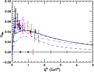
Figure 3: The neutron electric form factor $G_{En}$. Data are plotted as follows. Blue ($\times$)-ref. Pa99 , open blue circles ($\circ$)-ref. Os99 ; herberg , filled blue triangle-ref. Be99 , filled black square-ref.zhu , magenta diamond-ref.Ro99 . The black pluses (+) are extracted from elastic $ed$ polarization and cross section measurements by ref. Sc01 . Red filled circles-ref. madey . The black open circles-ref day on the baseline represent anticipated JLab Hall C data under analysis, and the red points along the baseline-ref. Ca02 are projected data, including statistics for JLab approved experiment in JLab Hall A. The projections to higher $Q^{2}$ planned for Hall A with the 12 GeV upgrade will extend these measurements to at least $Q^{2}\sim 5$ GeV²/c². The solid black curve is the present prediction The blue dashed curve is due to ref. miller due to constituent quarks and a pion cloud, while the blue dot-dash is from quarks only. The curve denoted by black dashes is the Galster galster parameterization.

The result for $G_{Mn}$ are shown in Fig. 4. Here, the fit to the experimental data is somewhat poorer than for $G_{En}$. Also shown is the result of the calculation of ref. miller . Curves are shown for two of the many parameter sets which fit the data. A possible reason for the better fit may be that ref. miller chooses parameters in such a way that requires the fit to be rather good for all four elastic form factors, while in the present case only the proton form factors are fit, and then isospin symmetry is applied to obtain the neutron form factors with the parameters fixed.

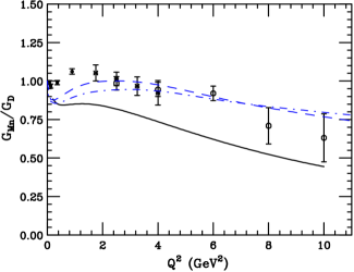
Figure 4: The neutron magnetic form factor $G_{Mn}$. The data are as follows. Small circles for $Q^{2}<1$ GeV²/c² ref. kubon . asterisks from $Q^{2}=$ 1.57 to 5 GeV²/c² ref. lung . Large circles for $Q^{2}=$ 2.5 to 10 GeV²/c² ref. rock . The solid curve is the prediction based on the present analysis. The blue dashed and dot-dashed curves are due to ref. miller for two different sets of parameters.

This note has pointed out the usefulness of GPDs in describing elastic form factors. Alternatively, the elastic form factors, together with isospin symmetry can be very important for constraining nucleon structure through GPDs. Further constraints of details of nucleon structure will be possible by including other high $-t$ experiments into the fit procedure. These include high $W$ high $-t$ real and virtual Compton scattering, and single meson photo and electroproduction, such as described in refs. rad_wacs ; kroll ; kroll_huang . It would be quite interesting if conceptual connections could be made between this technique and those of recent relativistic constituent quark models with a pion cloud such as in ref. miller , or recent helicity non-conserving pQCD based approaches ref. ralston ; belitsky which have had some success in explaining the $Q^{2}$ dependence of $F_{2p}$.

Acknowledgments: The work was partially supported by the National Science Foundation.

References

- (1) X. Ji, Phys. Rev. Lett. 78, 610 (1997).
- (2) A.V. Radyushkin, Phys. Lett. B380,417 (1996); Phys. Rev. D56,5524 (1997).
- (3) J. Collins, L. Frankfurt, and M. Strikman, Phys. Rev., D56, 2982 (1997).
- (4) A.V. Radyushkin, Phys. Rev. D58,114008 (1998).
- (5) M. Diehl, Th. Feldmann, R. Jakob and P. Kroll, Eur. Phys. C8, 409 (1999); M. Diehl, Th. Feldmann, R. Jakob and P. Kroll, Nucl. Phys. B596, 33 (2001), Erratum-ibid. B605, 647 (2001).
- (6) P. Kroll, Proceedings of the Workshop on Exclusive Processes at High Momentum Transfer, A. Radyushkin and P. Stoler, eds., World Scientific, Singapore, 214 (2003), E-print: hep-ph/0207118.
- (7) M. Burkardt, Proceedings of the Workshop on Exclusive Processes at High Momentum Transfer, A. Radyushkin and P. Stoler, eds., World Scientific, Singapore, 99 (2003), and references within.
- (8) P. Stoler, Phys. Rev. D65, 053013 (2002),hep-ph/0207312.
- (9) A. Afanasev, E-print: hep-ph/9910565; “Proceeding of the JLAB-INT Workshop on Exclusive and Semi-Exclusive Processes at High Momentum Transfer”, C. Carson and A. Radyushkin, eds. World Scientific (2000). May 1999
- (10) M.K. Jones et al. Phys. Rev. Lett. 84,1398 (2000);
- (11) O. Gayou et al. Phys. Rev. C64,038202 (2001).
- (12) A.D. Martin et al., Phys.Lett.B53,216,(2002).
- (13) P. Stoler, hep-ph/0210184.
- (14) E.J. Brash et al., Phys. Rev. C65, 051001(R) (2002).
- (15) R.G. Arnold et al., Phys. Rev. Lett. 57, 174 (1986).
- (16) L. Andivahis et al., Phys. Rev. D50, 5491 (1994).
- (17) H. Zhu et al., Phys. Rev. Lett. 87, 081801 (2001).
- (18) R. Madey et al. to be published.
- (19) G. A. Miller, Phys. Rev.c66, 032201 (2002), nucl-th/0207007.
- (20) S. Galster, H. Klein, J. Moritz, K.H. Schmidt, D. Wegener, Nucl. Phys. B32, 221 (1971).
- (21) I. Passchier et al., Phys. Rev. Lett. 82, 4988 (1999).
- (22) M. Ostrick et al., Phys. Rev. Lett. 83, 276 (1999).
- (23) C. Herberg et al., Eur. Phys. J. A 5, 131 (1999).
- (24) J. Becker et al., Eur. Phys. J. A 6, 329 (1999).
- (25) D. Rohe et al., Phys. Rev. Lett. 83, 4257 (1999).
- (26) R. Schiavilla and I. Sick, Phys. Rev. C 64, 041002 (2001).
- (27) Jefferson Lab Experiment E93-026, D. Day, G. Warren and M. Zeier, spokespersons, data under analysis.
- (28) Jefferson Lab Experiment E02-013, G. Cates, K. McCormick, B. Reitz and B. Wojtsekhowski, spokepersons.
- (29) G. Kubon et al. Phys.Lett.B524:26-32,2002,nucl-ex/0107016.
- (30) A. Lung et al., Phys. Rev. Lett. 70, 718 (1993).
- (31) S. Rock et al., Phys. Rev. Lett. 49, 1139 (1982).
- (32) H.W. Huang and P. Kroll, Eur. Phys. J. C17, w23 (2000).
- (33) Pankaj Jain and John P. Ralston, hep-ph/0306194.
- (34) A.V. Belitsky, X. Ji, F. Yuan hep-ph/0302043.