Generalized Parton Distributions and composite constituent quarks

Abstract

An approach is proposed to calculate Generalized Parton Distributions (GPDs) in a Constituent Quark Model (CQM) scenario, considering the constituent quarks as complex systems. The GPDs are obtained from the wave functions of the non relativistic CQM of Isgur and Karl, convoluted with the GPDs of the constituent quarks themselves. The latter are modelled by using the structure functions of the constituent quark, the double distribution representation of GPDs, and a recently proposed phenomenological constituent quark form factor. The present approach permits to access a kinematical range corresponding to both the DGLAP and the ERBL regions, for small values of the momentum transfer and of the skewedness parameter. In this kinematical region, the cross sections relevant to deeply virtual Compton scattering could be estimated by using the obtained GPDs. As an example, the leading twist, unpolarized GPD $H$ has been calculated. Its general relations with the non relativistic definition of the electric form factor and with the leading twist unpolarized quark density are consistently recovered from our expressions. Further natural applications of the proposed approach are addressed.

I Introduction

Generalized Parton Distributions (GPDs) [1] parametrize the non-perturbative hadron structure in hard exclusive processes (for comprehensive reviews, see, e.g., [2, 3, 4, 5, 6, 7]). The measurement of GPDs would provide information which is usually encoded in both the elastic form factors and the usual Parton Distribution Functions (PDFs) and, at the same time, it would represent a unique way to access several crucial features of the structure of the nucleon [8, 9]. By measuring GPDs, a test of the Angular Momentum Sum Rule of the proton [10] could be achieved for the first time, determining the quark orbital angular momentum contribution to the proton spin [9, 11].

Besides, the possibility of obtaining, by means of GPDs measurements, information on the structure of the proton in the impact parameter [12, 13] and position [14, 15, 16] spaces, is being presently discussed.

Therefore, relevant experimental efforts to measure GPDs, by means of exclusive electron Deep Inelastic Scattering (DIS) off the proton, are likely to take place in the next few years [17, 18, 19].

In this scenario, it becomes urgent to produce theoretical predictions for the behavior of these quantities. Several calculations have been already performed by using different descriptions of hadron structure: bag models [20, 21], soliton models [4, 22], light-front [23] and Bethe Salpeter approaches [24], phenomenological estimates based on parametrizations of PDFs [25, 26]. Besides, an impressive effort has been devoted to study the perturbative QCD evolution [27, 28] of GPDs, and the GPDs at twist three accuracy [29].

Recently, calculations have been performed also in Constituent Quark Models (CQM) [30, 31]. The CQM has a long story of successful predictions in low energy studies of the electromagnetic structure of the nucleon. In the high energy sector, in order to compare model predictions with data taken in DIS experiments, one has to evolve, according to perturbative QCD, the leading twist component of the physical structure functions obtained at the low momentum scale associated with the model, the so called “hadronic scale”, $\mu_{0}^{2}$.

Such a procedure, already addressed in [32, 33], has proven successful in describing the gross features of standard PDFs by using different CQM (see, e.g., [34]). Similar expectations motivated the study of GPDs in Ref. [30]. In that paper, a simple formalism has been proposed to calculate the quark contribution to GPDs from any non relativistic or relativized model and, as an illustration, results obtained in the Isgur and Karl model [35] have been evolved from $\mu_{0}^{2}$ up to DIS scales, to NLO accuracy. In Ref. [31] the same quark contribution to GPDs has been evaluated, at $\mu_{0}^{2}$, using the overlap representation of GPDs [6] in light-front dynamics, along the lines developed in [36].

In here, the procedure of Ref. [30] is extended and generalized. As a matter of fact, the approach of Ref. [30], when applied in the standard forward case, has been proven to reproduce the gross features of PDFs [34] but, in order to achieve a better agreement with data, it has to be improved. In a series of papers, it has been shown that unpolarized [37] and polarized [38] DIS data are consistent with a low energy scenario, dominated by complex constituent quarks inside the nucleon, defined through a scheme suggested by Altarelli, Cabibbo, Maiani and Petronzio (ACMP) [39], updated with modern phenomenological information. The same idea has been recently applied to demonstrate the evidence of complex objects inside the nucleon [40], analyzing intermediate energy data of electron scattering off the proton. Besides, a similar scenario has been extensively used by other groups, starting form the concept of “valon”, introduced more than twenty years ago [41] (for recent developments, see [42]).

We here generalize our description of the forward case [37] to the calculation scheme of Ref. [30], in order to obtain more realistic predictions for the GPDs and, at the same time, explore kinematical regions not accessible before.

In particular, the evaluation of the sea quark contribution becomes possible, so that GPDs could be calculated, in principle, in their full range of definition. Such an achievement would permit to estimate the cross-sections which are relevant for actual GPDs measurements, providing us with an important tool for planning future experiments. Actually, as it will be shown, the proposed approach will be applied here in a Non Relativistic (NR) framework, which allows one to evaluate the GPDs only for small values of the 4-momentum transfer, $\Delta^{2}$ (corresponding to $\vec{\Delta}^{2}\ll m^{2}$, where $m$ is the constituent quark mass) and small values also for the skewedness parameter, $\xi$. The full kinematical range of definition of GPDs will be studied in a followup, introducing relativity in the scheme.

The paper is structured as follows. After the definition of the main quantities of interest, an Impulse Approximation (IA) convolution formula for the current quark GPDs in terms of the constituent quark off-diagonal momentum distributions and constituent quark GPDs is derived in the third section. Then, the constituent quark GPDs are built in the fourth section, according to ACMP philosophy and using the Double Distribution (DD’s) representation [3, 26, 43] of the GPDs. In the fifth section, as an illustration, results obtained by using CQM wave functions of the IK model and the obtained constituent quark GPDs will be shown. Conclusions will be drawn in the last section.

II Quark Model Calculations of GPDs

We are interested in hard exclusive processes. The absorption of a high-energy virtual photon by a quark in a hadron target is followed by the emission of a particle to be later detected; finally, the interacting quark is reabsorbed back into the recoiling hadron. If the emitted and detected particle is, for example, a real photon, the so called Deeply Virtual Compton Scattering process takes place [8, 9, 11]. We adopt here the formalism used in Ref. [2]. Let us think to a nucleon target, with initial (final) momentum and helicity $P(P^{\prime})$ and $s(s^{\prime})$, respectively. The GPDs $H_{q}(x,\xi,\Delta^{2})$ and $E_{q}(x,\xi,\Delta^{2})$ are defined through the expression

$$F^{q}_{s^{\prime}s}(x,\xi,\Delta^{2}) = {1\over 2}\int{d\lambda\over 2\pi}e^{i\lambda x}\langle P^{\prime}s^{\prime}|\,\bar{\psi}_{q}\left(-{\lambda n\over 2}\right)n/\,\psi_{q}\left({\lambda n\over 2}\right)|Ps\rangle=$$ (1)

$$= H_{q}(x,\xi,\Delta^{2}){1\over 2}\bar{U}(P^{\prime},s^{\prime})n/U(P,s)+E_{q}(x,\xi,\Delta^{2}){1\over 2}\bar{U}(P^{\prime},s^{\prime}){i\sigma^{\mu\nu}n_{\mu}\Delta_{\nu}\over 2M}U(P,s)~{},$$ (2)

where $\Delta=P^{\prime}-P$ is the 4-momentum transfer to the nucleon, $\psi_{q}$ is the quark field and M is the nucleon mass. It is convenient to work in a system of coordinates where the photon 4-momentum, $q^{\mu}=(q_{0},\vec{q})$, and $\bar{P}=(P+P^{\prime})/2$ are collinear along $z$. The $\xi$ variable in the arguments of the GPDs is the so called “skewedness”, parametrizing the asymmetry of the process. It is defined by the relation $\xi=-n\cdot\Delta/2$, where $n$ is a light-like 4-vector satisfying the condition $n\cdot\bar{P}=1$. As explained in [9, 11], GPDs describe the amplitude for finding a quark with momentum fraction $~{}~{}x+\xi$ (in the Infinite Momentum Frame) in a nucleon with momentum $(1+\xi)\bar{P}$ and replacing it back into the nucleon with a momentum transfer $\Delta$. Besides, when the quark longitudinal momentum fraction $x$ of the average nucleon momentum $\bar{P}$ is less than $-\xi$, GPDs describe antiquarks; when it is larger than $\xi$, they describe quarks; when it is between $-\xi$ and $\xi$, they describe $q\bar{q}$ pairs. The first and second case are commonly referred to as DGLAP region and the third as ERBL region [2], following the pattern of evolution in the factorization scale. One should keep in mind that, besides the variables $x,\xi$ and $\Delta^{2}$ explicitly shown, GPDs depend, as the standard PDFs, on the momentum scale $Q^{2}$ at which they are measured or calculated. For an easy presentation, this latter dependence will be omitted in the rest of the paper, unless specifically needed. The values of $\xi$ which are possible for a given value of $\Delta^{2}$ are:

$$0\leq\xi\leq\sqrt{-\Delta^{2}}/\sqrt{4M^{2}-\Delta^{2}}~{}.$$ (3)

The well known natural constraints of $H_{q}(x,\xi,\Delta^{2})$ are:

i) the so called “forward” or “diagonal” limit, $P^{\prime}=P$, i.e., $\Delta^{2}=\xi=0$, where one recovers the usual PDFs

$$H_{q}(x,0,0)=q(x)~{};$$ (4)

ii) the integration over $x$, yielding the contribution of the quark of flavor $q$ to the Dirac form factor (f.f.) of the target:

$$\int dxH_{q}(x,\xi,\Delta^{2})=F_{1}^{q}(\Delta^{2})~{};$$ (5)

iii) the polynomiality property [2], involving higher moments of GPDs, according to which the $x$-integrals of $x^{n}H^{q}$ and of $x^{n}E^{q}$ are polynomials in $\xi$ of order $n+1$.

In [30], the IA expression for $H_{q}(x,\xi,\Delta^{2})$, suitable to perform CQM calculations, has been obtained.

Now, it will be shown that the same basic formula can be derived as the NR reduction of the definition (1) of GPDs, analyzed initially in the non-covariant framework of light-cone quantization, involving partons on their mass shell.

Using the light-cone spinor definitions as given in the appendix B of [5], and defining: $k^{+}=(k_{0}+k_{3})/\sqrt{2},\vec{k}_{\perp}=(k_{1},k_{2})$, for the light-cone helicity combination $s^{\prime}s={1\over 2}{1\over 2}=++$ one obtains

$$F^{q}_{++}(x,\xi,\Delta^{2})={\sqrt{1-\xi^{2}}}H_{q}(x,\xi,\Delta^{2})-{\xi^{2}\over\sqrt{1-\xi^{2}}}E_{q}(x,\xi,\Delta^{2})~{},$$ (6)

so that, for $\xi^{2}\ll 1$:

$$F^{q}_{++}(x,\xi,\Delta^{2})={H_{q}(x,\xi,\Delta^{2})}-\xi^{2}\left({1\over 2}H_{q}(x,\xi,\Delta^{2})+E_{q}(x,\xi,\Delta^{2})\right)+O(\xi^{4})~{},$$ (7)

i.e.

$$F^{q}_{++}(x,\xi,\Delta^{2})=H_{q}(x,\xi,\Delta^{2})+O(\xi^{2})~{}.$$ (8)

The reader should be aware that the so called “Munich Symmetry” for double distributions excludes $O(\xi)$ contributions to GPDs [44], so that the accuracy of the above equation is worse than it reads.

According to the latter equation, in order to obtain the GPD $H_{q}(x,\xi,\Delta^{2})$ for $\xi^{2}\ll 1$ one has to evaluate $F_{++}^{q}$, starting from its definition, Eq (1). In the l.h.s. of the latter, using light-cone quantized quark fields, whose creation and annihilation operators, $b^{\dagger}(k)$ and $b(k)$, obey the commutation relation

$$\{b(k^{\prime}),b^{\dagger}(k)\}=(2\pi)^{3}2k^{+}\delta(k^{\prime+}-k^{+})\delta^{2}(\vec{k}_{\perp}-\vec{k}_{\perp}^{\prime})~{},$$ (9)

and using properly normalized light-cone states

$$\langle P^{\prime}|P\rangle=(2\pi)^{3}2P^{+}\delta(P^{\prime+}-P^{+})\delta^{2}(\vec{P}_{\perp}-\vec{P}_{\perp}^{\prime})~{},$$ (10)

one obtains, for $x>\xi$ [2]

$$F^{q}_{++}(x,\xi,\Delta^{2})={1\over 2\bar{P}^{+}V}\int{d^{2}k_{\perp}\over 2\sqrt{|x^{2}-\xi^{2}|}(2\pi)^{3}}\langle b^{\dagger}(k+\Delta)b(k)\rangle~{},$$ (11)

where

$$\langle b^{\dagger}(k^{\prime})b(k)\rangle=\sum_{\lambda}\langle P^{\prime}+|b_{\lambda}^{\dagger}((x-\xi)\bar{P}^{+},{\vec{k}_{\perp}^{\prime}})b_{\lambda}((x+\xi)\bar{P}^{+},{\vec{k}_{\perp}})|P+\rangle~{},$$ (12)

and $V$ is a volume factor. We are interested here in the $x>\xi$ region, since we want to obtain only the quark contribution to $H$, the only one which can be evaluated in a CQM with three valence, point-like quarks.

Eq. (11) can be written:

$$F^{q}_{++}(x,\xi,\Delta^{2}) = {1\over 2\bar{P}^{+}V}\int{d^{2}k_{\perp}\over 2\sqrt{|x^{2}-\xi^{2}|}(2\pi)^{3}}\langle b^{\dagger}(k+\Delta)b(k)\rangle=$$ (13)

$$= {1\over 2\bar{P}^{+}V}\int{d^{2}k_{\perp}dk^{+}\over 2\sqrt{|x^{2}-\xi^{2}|}(2\pi)^{3}}\delta(k^{+}-(x+\xi)\bar{P}^{+})\langle b^{\dagger}(k+\Delta)b(k)\rangle=$$ (14)

$$= {1\over 2\bar{P}^{+}V}\int{d^{2}k_{\perp}dk^{+}\over 2\sqrt{(x+\xi)\bar{P}^{+}(x-\xi)\bar{P}^{+}}(2\pi)^{3}}\bar{P}^{+}\times$$ (15)

$$\times \delta(k^{+}-(x+\xi)\bar{P}^{+})\langle b^{\dagger}(k+\Delta)b(k)\rangle=$$ (16)

$$= {1\over 2\bar{P}^{+}V}\int{d^{2}k_{\perp}dk^{+}\over 2\sqrt{k^{+}k^{\prime+}}(2\pi)^{3}}\delta\left({k^{+}\over\bar{P}^{+}}-(x+\xi)\right)\langle b^{\dagger}(k+\Delta)b(k)\rangle~{}.$$ (17)

In a NR framework, states and creation and annihilation operators have to be normalized according to

$$\langle\vec{P}^{\prime}|\vec{P}\rangle=(2\pi)^{3}\delta(P^{\prime+}-P^{+})\delta(\vec{P}^{\prime}_{\perp}-\vec{P}_{\perp})~{}$$ (18)

and

$$\{b(k^{\prime+},\vec{k}_{\perp}),b^{\dagger}(k^{+},\vec{k}^{\prime}_{\perp})\}=(2\pi)^{3}\delta(k^{\prime+}-k^{+})\delta(\vec{k}^{\prime}_{\perp}-\vec{k}_{\perp})~{}$$ (19)

respectively. As a consequence, in order to perform a NR reduction of Eq. (17), one has to consider that [45]:

$$|P\rangle\rightarrow\sqrt{2P^{+}}|\vec{P}\rangle~{},$$ (20)

$$b(k)\rightarrow\sqrt{2k^{+}}b(k^{+},\vec{k}_{\perp})~{},$$ (21)

so that in Eq. (17), in terms of the new states and fields, one has to perform the substitution

$$\langle b^{\dagger}(k+\Delta)b(k)\rangle = \sum_{\lambda}\langle P^{\prime}+|b_{\lambda}^{\dagger}((x-\xi)\bar{P}^{+},\vec{k}_{\perp}+\vec{\Delta}_{\perp})b_{\lambda}((x+\xi)\bar{P}^{+},\vec{k}_{\perp})|P+\rangle\rightarrow$$ (22)

$$\rightarrow 2\sqrt{1-\xi^{2}}\bar{P}^{+}\sqrt{2k^{\prime+}2k^{+}}\sum_{\lambda}\langle\vec{P}^{\prime}|b_{\lambda}^{\dagger}(k^{+}+\Delta^{+},\vec{k}_{\perp}+\vec{\Delta}_{\perp})b_{\lambda}(k^{+},\vec{k}_{\perp})|\vec{P}\rangle~{},$$ (23)

where use has been made of the relation $2\sqrt{1-\xi^{2}}\bar{P}^{+}=\sqrt{2P^{+}}\sqrt{2P^{\prime+}}$.

Now, inserting Eq. (23) in Eq. (17), one gets

$$F_{++}^{q}(x,\xi,\Delta^{2}) = {1\over V}\int{d^{2}k_{\perp}dk^{+}\over 2\sqrt{k^{+}k^{\prime+}}(2\pi)^{3}}\delta\left({k^{+}\over\bar{P}^{+}}-(x+\xi)\right)\times$$ (24)

$$\times \sqrt{2k^{\prime+}2k^{+}}\sum_{\lambda}\langle\vec{P}^{\prime}|b_{\lambda}^{\dagger}(k^{+}+\Delta^{+},\vec{k}_{\perp}+\vec{\Delta}_{\perp})b_{\lambda}(k^{+},\vec{k}_{\perp})|\vec{P}\rangle+O(\xi^{2})=$$ (25)

$$= {1\over V}\int{d^{2}k_{\perp}dk^{+}\over(2\pi)^{3}}\delta\left({k^{+}\over\bar{P}^{+}}-(x+\xi)\right)\times$$ (26)

$$\times \sum_{\lambda}\langle\vec{P}^{\prime}|b_{\lambda}^{\dagger}(k^{+}+\Delta^{+},\vec{k}_{\perp}+\vec{\Delta}_{\perp})b_{\lambda}(k^{+},\vec{k}_{\perp})|\vec{P}\rangle+O(\xi^{2})~{}.$$ (27)

Now, since the constituent quarks with mass $m$ are taken to be on shell, so that $k_{0}=\sqrt{\vec{k}^{2}+m^{2}}$, one has

$$d^{2}k_{\perp}dk^{+}\rightarrow\left({k^{+}\over k_{0}}\right)d\vec{k}~{},$$ (28)

so that, from Eq. (27) and Eq. (8), one gets:

$$H_{q}(x,\xi,\Delta^{2}) = \int{d\vec{k}}\,\,\delta\left({k^{+}\over\bar{P}^{+}}-(x+\xi)\right)\times$$ (29)

$$\times \left[{1\over(2\pi)^{3}V}{k^{+}\over k_{0}}\sum_{\lambda}\langle\vec{P}^{\prime}|b_{\lambda}^{\dagger}(k^{+}+\Delta^{+},\vec{k}_{\perp}+\vec{\Delta}_{\perp})b_{\lambda}(k^{+},\vec{k}_{\perp})|\vec{P}\rangle\right]+O(\xi^{2})=$$ (30)

$$= \int d\vec{k}\,\,\delta\left({k^{+}\over\bar{P}^{+}}-(x+\xi)\right)\left[\,n_{q}(\vec{k},\vec{k}+\vec{\Delta})+O\left({\vec{k}^{2}\over m^{2}},{(\vec{k}+\vec{\Delta})^{2}\over m^{2}}\right)\,\right]+O(\xi^{2})~{}.$$ (31)

In the last step, the definition of (non-diagonal) momentum distribution, $\,n_{q}(\vec{k},\vec{k}+\vec{\Delta})$, has been used, together with the fact that a NR momentum distribution describes the probability of finding a constituent of momentum $\vec{k}$ in a given system up to terms of order ${\vec{k}^{2}\over m^{2}}$ [46].

Summarizing, we find that, in a NR CQM, the GPD $H_{q}(x,\xi,\Delta^{2})$ can be calculated, for $\xi^{2}\ll 1$, $\vec{k}^{2}\ll m^{2}$ and $(\vec{k}+\vec{\Delta})^{2}\ll m^{2}$ (which means, in turn, $\vec{\Delta}^{2}\ll m^{2}$), through the following expression:

$$H_{q}(x,\xi,\Delta^{2})=\int d\vec{k}\,\delta\left({k^{+}\over\bar{P}^{+}}-(x+\xi)\right)\,n_{q}(\vec{k},\vec{k}+\vec{\Delta})+O\left(\xi^{2},{\vec{k}^{2}\over m^{2}},{\vec{\Delta}^{2}\over m^{2}}\,\right)~{}.$$ (32)

The above equation, corresponding to Eq. (8) in [30], permits the calculation of $H_{q}(x,\xi,\Delta^{2})$ in any CQM, and it naturally verifies some of the properties of GPDs. In fact, the unpolarized quark density, $q(x)$, as obtained by analyzing, in IA, DIS off the nucleon (see, e.g., [45]), assuming that the interacting quark is on-shell, is recovered in the forward limit, where $\Delta^{2}=\xi=0$:

$$q(x)=H_{q}(x,0,0)=\int d\vec{k}\,n_{q}(\vec{k})\,\delta\left(x-{k^{+}\over\bar{P}^{+}}\right)~{},$$ (33)

so that the constraint Eq. (4) is fulfilled. In the above equation, $n_{q}(\vec{k})$ is the momentum distribution of the quarks in the nucleon:

$$n_{q}(\vec{k})=\int e^{i\vec{k}\cdot(\vec{r}-\vec{r}^{\prime})}\rho_{q}(\vec{r},\vec{r}^{\prime})d\vec{r}d\vec{r}^{\prime}~{}.$$ (34)

Besides, integrating Eq. (32) over $x$, one obtains

$$\int dxH_{q}(x,\xi,\Delta^{2})=\int d\vec{r}e^{i\vec{\Delta}\cdot\vec{r}}\rho_{q}(\vec{r})~{},$$ (35)

where $\rho_{q}(\vec{r})=\lim_{\vec{r}^{\prime}\rightarrow\vec{r}}\rho_{q}(\vec{r}^{\prime},\vec{r})$ is the contribution of the quark $q$ to the charge density. The r.h.s. of the above equation gives the IA definition of the charge f.f.

$$\int d\vec{r}e^{i\vec{\Delta}\cdot\vec{r}}\rho_{q}(\vec{r})=F^{q}(\Delta^{2})~{},$$ (36)

so that, recalling that $F^{q}(\Delta^{2})$ coincides with the non relativistic limit of the Dirac f.f. $F_{1}^{q}(\Delta^{2})$, Eq. (5) is verified.

Besides, the polynomiality condition is formally fulfilled by the GPD defined in Eq. (32), although the present accuracy of the model, explicitly written in the latter equation, does not allow to really check polynomiality, due to the already mentioned effects of the Munich Symmetry [44].

The definition of $H_{q}(x,\xi,\Delta^{2})$ in terms of CQM wave functions can be generalized to other GPDs, and the relation of the latter quantities with other form factors (for example the magnetic one) and other PDFs (for example the polarized quark density) can be recovered. Therefore the proposed scheme allows one to calculate the GPDs by using any CQM.

With respect to Eq. (32), a few caveats are necessary.

i) One should keep in mind that Eq. (32) is a NR result, holding for $\xi^{2}\ll 1$, under the conditions $\vec{k}^{2}\ll m^{2}$, $\vec{\Delta}^{2}\ll m^{2}$. If one wants to treat more general processes, the NR limit should be relaxed by taking into account relativistic corrections. In this way, at the same time, an expression to evaluate $E_{q}(x,\xi,\Delta^{2})$ could be obtained. Since our main aim here is to describe our approach, rather than to obtain realistic estimates, we postpone to a later publication the discussion of a relativistic model, which will permit to study the full $\Delta^{2}$- and $\xi$-range, together with the GPD $E_{q}(x,\xi,\Delta^{2})$.

ii) The Constituent Quarks are assumed to be point-like.

iii) If use is made of a CQM, containing only constituent quarks (and also antiquarks in the case of mesons), only the quark (and antiquark) contribution to the GPDs can be evaluated, i.e., only the region $x\geq\xi$ (and also $x\leq-\xi$ for mesons) can be explored. In order to introduce the study of the ERBL region ($-\xi\leq x\leq\xi$), so that observables like cross-sections, spin asymmetries and so on can be calculated, the model has to be enriched.

iv) In actual calculations, the evaluation of Eq. (32) requires the choice of a reference frame. In the following, the Breit Frame will be chosen, where one has $\Delta^{2}=-\vec{\Delta}^{2}$ and, in the NR limit we are studying, one finds $\sqrt{2}\bar{P}^{+}\rightarrow M$. It happens therefore that, in the argument of the $\delta$ function in Eq. (32), the $x$ variable for the valence quarks is not defined in its natural support, i.e. it can be larger than 1 and smaller than $\xi$. Several prescriptions have been proposed in the past to overcome such a difficulty in the standard PDFs case [33, 34]. Although the support violation is small for the calculations that will be shown here, it has to be reported as a drawback of the approach.

The issue iii) will be discussed in the next sections, by relaxing the condition ii) and allowing for a finite size and composite structure of the constituent quark.

III GPDs in a Constituent Quark Scenario

The procedure described in the previous section, when applied in the standard forward case, has been proven to be able to reproduce the gross features of PDFs [34]. In order to achieve a better agreement with data, the approach has to be improved.

In a series of previous papers, it has been shown that unpolarized [37] and polarized [38] DIS data are consistent with a low energy scenario dominated by composite constituents of the nucleon. This was obtained using a simple picture of the constituent quark as a complex system of point-like partons, and thus constructing the forward parton distributions by a convolution between constituent quark momentum distributions and constituent quark structure functions. The latter quantities were obtained by using updated phenomenological information in a scenario firstly suggested by Altarelli, Cabibbo, Maiani and Petronzio (ACMP) already in the seventies [39].

Following the same idea, in this section a model for the reaction mechanism of an off-forward process, such as DVCS, where GPDs could be measured, will be proposed. As a result, a convolution formula giving the proton $H_{q}$ GPD in terms of a constituent quark off-forward momentum distribution, $H_{q_{0}}$, and of a GPD of the constituent quark $q_{0}$ itself, $H_{q_{0}q}$, will be derived.

It is assumed that the hard scattering with the virtual photon takes place on a parton of a spin $1/2$ target, made of complex constituents. This can be the case of a spin $1/2$ nucleus, such as ${}^{3}He$, or of the proton, if this is assumed to be made of composite constituent quarks. The latter situation is the one we are interested in.

The scenario we are thinking of is depicted in Fig. 1 for the special case of DVCS, in the handbag approximation. One parton (current quark) with momentum $k$, belonging to a given constituent of momentum p, interacts with the probe and it is afterwards reabsorbed, with momentum $k+\Delta$, by the same constituent, without further re-scattering with the recoiling system of momentum $P_{R}$. We suggest here an analysis of the process which is quite similar to the usual IA approach to DIS off nuclei [45, 46, 47].

In the class of frames chosen in section 2, and in addition to the kinematical variables, $x$ and $\xi$, already defined, one needs a few more to describe the process. In particular, $x^{\prime}$ and $\xi^{\prime}$, for the “internal” target, i.e., the constituent quark, have to be introduced. The latter quantities can be obtained defining the “+” components of the momentum $k$ and $k+\Delta$ of the struck parton before and after the interaction, with respect to $\bar{P}^{+}$ and $\bar{p}^{+}={1\over 2}(p+p^{\prime})^{+}$:

$$k^{+} = (x+\xi)\bar{P}^{+}=(x^{\prime}+\xi^{\prime})\bar{p}^{+}~{},$$ (37)

$$(k+\Delta)^{+} = (x-\xi)\bar{P}^{+}=(x^{\prime}-\xi^{\prime})\bar{p}^{+}~{}.$$ (38)

From the above expressions, $\xi^{\prime}$ and $x^{\prime}$ are immediately obtained as

$$\xi^{\prime} = -{\Delta^{+}\over 2\bar{p}^{+}}$$ (39)

$$x^{\prime} = {\xi^{\prime}\over\xi}x$$ (40)

and, since $\xi=-\Delta^{+}/(2\bar{P}^{+})$, if $\tilde{z}=p^{+}/P^{+}$, one also has

$$\xi^{\prime}={\xi\over\tilde{z}(1+\xi)-\xi}~{}.$$ (41)

These expressions have been already found and used in the IA analysis of DVCS off the deuteron [48] and, in general, off nuclei [49].

In order to derive a convolution formula, a standard procedure will be adopted [45, 46, 47]. In Eq. (30), two complete sets of states, corresponding to the interacting constituent and to the recoiling system, are properly inserted to the left and right-hand sides of the quark operator:

$${H_{q}(x,\xi,\Delta^{2})} = {\langle P^{\prime}+|}\,\,\sum_{\vec{P}_{R}^{\prime},S_{R}^{\prime},\vec{p}^{\prime},s^{\prime}}{\{|P_{R}^{\prime}S_{R}^{\prime}\rangle|p^{\prime}s^{\prime}\rangle\}}\{\langle P_{R}^{\prime}S_{R}^{\prime}|{\langle p^{\prime}s^{\prime}|}\}$$ (44)

$$\int{d\vec{k}\over(2\pi)^{3}}{k^{+}\over k_{0}}\delta\left({k^{+}\over\bar{P}^{+}}-(x+\xi)\right){1\over V}\sum_{\lambda}b_{\lambda}^{\dagger}(\vec{k}+\vec{\Delta})b_{\lambda}(\vec{k})$$

$$\sum_{\vec{P}_{R},S_{R},\vec{p},s}\{|P_{R}S_{R}\rangle{|ps\rangle\}}{\{\langle P_{R}S_{R}|\langle ps|\}\,\,\,\,|P+\rangle}~{},$$

and since, using IA,

$${\{\langle P_{R}S_{R}|\langle ps|\}|PS\rangle}={\langle P_{R}S_{R},ps|PS\rangle}(2\pi)^{3}\delta^{3}(\vec{P}-\vec{P}_{R}-\vec{p})\delta_{S,S_{R}\,s}~{},$$ (45)

a convolution formula, valid for any GPD $H_{q}$ of the spin 1/2 complex target (the proton in the present case) in terms of the GPD $H_{q_{0}q}$ of spin 1/2 structured constituents (the constituent quark, in the present case), $q_{0}$, is readily obtained:

$$H_{q}(x,\xi,\Delta^{2}) = \sum_{q_{0}}\int dE\int d\vec{p}\,P_{q_{0}}(\vec{p},\vec{p}+\vec{\Delta},E){\xi^{\prime}\over\xi}H_{q_{0}q}(x^{\prime},\xi^{\prime},\Delta^{2})~{}.$$ (46)

In the above equation, $E$ is the excitation energy of the recoiling system and $P_{q_{0}}(\vec{p},\vec{p}+\vec{\Delta},E)$ the one-body off-diagonal spectral function for the constituent quark $q_{0}$ in the proton:

$$P_{q_{0}}(\vec{p},\vec{p}+\vec{\Delta},E)=\sum_{\vec{S}_{R},s}\langle\vec{P}^{\prime}S|(\vec{P}-\vec{p})S_{R},(\vec{p}+\vec{\Delta})s\rangle\langle(\vec{P}-\vec{p})S_{R},\vec{p}s|\vec{P}S\rangle\,\delta(E-E_{R})~{}.$$ (47)

If the $E$-dependence of $\xi^{\prime}$, i.e., the $E$-dependence of $\tilde{z}$ (cf. Eq. (41)) is disregarded in Eq. (46), so that the one-body off-diagonal momentum distribution

$$n_{q_{0}}(\vec{p},\vec{p}+\vec{\Delta})=\int dEP_{q_{0}}(\vec{p},\vec{p}+\vec{\Delta},E)~{}$$ (48)

is recovered, Eq.(46) can be written in the form

$$H_{q}(x,\xi,\Delta^{2}) \simeq \sum_{q_{0}}\int d\vec{p}\,n_{q_{0}}(\vec{p},\vec{p}+\vec{\Delta}){\xi^{\prime}\over\xi}H_{q_{0}q}(x^{\prime},\xi^{\prime},\Delta^{2})=$$ (49)

$$= \sum_{q_{0}}\int_{x}^{1}{dz\over z}\int d\vec{p}\,n_{q_{0}}(\vec{p},\vec{p}+\vec{\Delta})\delta\left(z-{\xi\over\xi^{\prime}}\right)H_{q_{0}q}\left({x\over z},{\xi\over z},\Delta^{2}\right)~{}.$$ (50)

Taking into account that

$$z-{\xi\over\xi^{\prime}}=z-[\tilde{z}(1+\xi)-\xi]=z+\xi-{p^{+}\over P^{+}}(1+\xi)=z+\xi-{p^{+}\over\bar{P}^{+}}~{},$$ (51)

Eq. (50) can also be written in the form:

$$H_{q}(x,\xi,\Delta^{2})=\sum_{q_{0}}\int_{x}^{1}{dz\over z}H_{q_{0}}(z,\xi,\Delta^{2})H_{q_{0}q}\left({x\over z},{\xi\over z},\Delta^{2}\right)~{},$$ (52)

where

$$H_{q_{0}}(z,\xi,\Delta^{2})=\int d\vec{p}\,n_{q_{0}}(\vec{p},\vec{p}+\vec{\Delta})\delta\left(z+\xi-{p^{+}\over\bar{P}^{+}}\right)$$ (53)

is to be evaluated in a given CQM, according to Eq. (32), for $q_{0}=u_{0}$ or $d_{0}$, while $H_{q_{0}q}({x\over z},{\xi\over z},\Delta^{2})$ is the constituent quark GPD, which is still to be discussed and will be modelled in the next section. One should notice that the forward limit of Eq. (52) gives the expression which is usually found, for the parton distribution $q(x)$, in the IA analysis of unpolarized DIS off nuclei [45, 46, 47]. In fact, if in Eq. (52) the index $q_{0}$, labelling a constituent quark, is replaced by the index $N$, labelling a nucleon in the nucleus, in the forward limit one finds the well known result:

$$q(x)=H_{q}(x,0,0)=\sum_{N}\int_{x}^{1}{dz\over z}f_{N}(z)\,q_{N}\left({x\over z}\right)~{},$$ (54)

where

$$f_{N}(z)=H_{N}(z,0,0)=\int d\vec{p}\,n_{N}(\vec{p})\delta\left(z-{p^{+}\over\bar{P}^{+}}\right)$$ (55)

is the light-cone momentum distribution of the nucleon $N$ in the nucleus and $q_{N}(x)=H_{Nq}(x,0,0)$ is the distribution of the quark of flavor $q$ in the nucleon $N$.

IV A model for the GPDs of the Constituent Quark

The crucial problem now is the definition of $H_{q_{0}q}({x\over z},{\xi\over z},\Delta^{2})$, the constituent quark GPD, appearing in Eq. (52).

As usual, we can start modelling this quantity thinking first of all to its forward limit, where the constituent quark parton distributions have to be recovered. As we said in the previous section, in a series of papers [37, 38] a simple picture of the constituent quark as a complex system of point-like partons has been proposed, re-taking a scenario suggested by Altarelli, Cabibbo, Maiani and Petronzio (ACMP) [39].

Let us recall the main features of that idea.

The constituent quarks are themselves composite objects whose structure functions are described by a set of functions $\phi_{q_{0}q}(x)$ that specify the number of point-like partons of type $q$ which are present in the constituent of type $q_{0}$, with fraction $x$ of its total momentum. We will hereafter call these functions, generically, the structure functions of the constituent quark.

The functions describing the nucleon parton distributions are expressed in terms of the independent $\phi_{q_{0}q}(x)$ and of the constituent density distributions ($q_{0}=u_{0},d_{0}$) as,

$$q(x,Q^{2})=\sum_{q_{0}}\int_{x}^{1}{dz\over z}q_{0}(z,Q^{2})\phi_{q_{0}q}\left({x\over z},Q^{2}\right)~{},$$ (56)

where $q$ labels the various partons, i.e., valence quarks ($u_{v},d_{v}$), sea quarks ($u_{s},d_{s},s$), sea antiquarks ($\bar{u},\bar{d},\ \bar{s}$) and gluons $g$.

The different types and functional forms of the structure functions of the constituent quarks are derived from three very natural assumptions [39]:

• The point-like partons are $QCD$ degrees of freedom, i.e. quarks, antiquarks and gluons;

• Regge behavior for $x\rightarrow 0$ and duality ideas;

• invariance under charge conjugation and isospin.

These considerations define in the case of the valence quarks the following structure function

$$\phi_{qq_{v}}({x},Q^{2})={\Gamma(A+{1\over 2})\over\Gamma({1\over 2})\Gamma(A)}{(1-x)^{A-1}\over\sqrt{x}}.$$ (57)

For the sea quarks the corresponding structure function becomes,

$$\phi_{qq_{s}}({x},Q^{2})={C\over x}(1-x)^{D-1},$$ (58)

and, in the case of the gluons, it is taken

$$\phi_{qg}({x},Q^{2})={G\over x}(1-x)^{B-1}~{}.$$ (59)

The last assumption of the approach relates to the scale at which the constituent quark structure is defined. We choose for it the so called hadronic scale $\mu_{0}^{2}$ [34, 50]. This hypothesis fixes $all$ the parameters of the approach (Eqs. (57) through (59)). The constants $A$, $B$, $G$ and the ratio $C/D$ are determined by the amount of momentum carried by the different partons, corresponding to a hadronic scale of $\mu_{0}^{2}=0.34$ GeV², according to the parametrization of [50]. $C$ (or $D$) is fixed according to the value of $F_{2}$ at $x=0.01$ [39], and its value is chosen again according to [50]. We stress that all these inputs are forced only by the updated phenomenology, through the 2^nd moments of PDFs. The values of the parameters obtained are listed in [37].

We, here, note that the unpolarized structure function $F_{2}$ is rather insensitive to the change of the sea ($C$, $D$) and gluon ($B$, $G$) parameters.

The other ingredients appearing in Eq. (56), i.e., the density distributions for each constituent quark, are defined according to Eq. (32).

Now we have to generalize this scenario to describe off-forward phenomena. Of course, the forward limit of our GPDs formula, Eq. (52), has to be given by Eq. (56). By taking the forward limit of Eq. (52), one obtains:

$$H_{q}(x,0,0) = \sum_{q_{0}}\int_{x}^{1}{dz\over z}H_{q_{0}}(z,0,0)H_{q_{0}q}\left({x\over z},0,0\right)$$ (60)

$$= \sum_{q_{0}}\int_{x}^{1}{dz\over z}q_{0}(z)H_{q_{0}q}\left({x\over z},0,0\right)~{},$$ (61)

so that, in order for the latter to coincide with Eq. (56), one must have $H_{q_{0}q}(x,0,0)\equiv\phi_{q_{0}q}(x)$.

In such a way, through the ACMP prescription, the forward limit of the unknown constituent quark GPD $H_{q_{0}q}({x\over z},{\xi\over z},\Delta^{2})$ can be fixed.

Now the off-forward behavior of the Constituent Quark GPDs has to be modelled.

This can be done in a natural way by using the “$\alpha$-Double Distributions” (DD’s) language proposed by Radyushkin [3, 43]. DD’s, $\Phi(\tilde{x},\alpha,\Delta^{2})$, are a representation of GPDs which automatically guarantees the polynomiality property. GPDs can be obtained from DD’s after a proper integration. In constructing models, the DD’s can represent a more appropriate language with respect to GPDs. In fact, the hybrid character of GPDs, which are something in between parton densities $q(x)$ and distribution amplitudes $\phi(\alpha)$, is naturally emphasized when the latter are obtained from DD’s. The DD’s do not depend on the skewedness parameter $\xi$; rather, they describe how the total, $P$, and transfer, $\Delta$, momenta are shared between the interacting and final partons, by means of the variables $\tilde{x}$ and $\alpha$, respectively. As it can be argued from Fig. 2, where the DDs representation of GPDs is illustrated schematically, and as it is explained in [3, 43], parton densities are recovered in the forward, $\Delta=0$ limit, while meson distribution amplitudes are obtained in the $P=0$ limit of DD’s. In some cases, such a transparent physical interpretation, together with the symmetry properties which are typical of distribution amplitudes ($\alpha\rightarrow-\alpha$ symmetry), allows a direct modelling, already developed in [26].

The relation between any GPD $H$, defined à la Ji, for example the one we need, i.e. $H_{q_{0}q}$ for the constituent quark target, is related to the $\alpha$-DD’s, which we call $\tilde{\Phi}_{q_{0}q}(\tilde{x},\alpha,\Delta^{2})$ for the constituent quark, in the following way [3, 43]:

$$H_{q_{0}q}(x,\xi,\Delta^{2})=\int_{-1}^{1}d\tilde{x}\int_{-1+|\tilde{x}|}^{1-|\tilde{x}|}\delta(\tilde{x}+\xi\alpha-x)\tilde{\Phi}_{q_{0}q}(\tilde{x},\alpha,\Delta^{2})d\alpha~{}.$$ (62)

With some care, the expression above can be integrated over $\tilde{x}$ and the result is explicitly given in [3]. The DDs fulfill the relation:

$$\tilde{\Phi}_{q_{0}q}(\tilde{x},\alpha,\Delta^{2})=\tilde{\Phi}_{q_{0}q}(\tilde{x},-\alpha,\Delta^{2})~{},$$ (63)

and the polynomiality condition [2].

In [43], a factorized ansatz is suggested for the DD’s:

$$\tilde{\Phi}_{q_{0}q}(\tilde{x},\alpha,\Delta^{2})=h_{q}(\tilde{x},\alpha,\Delta^{2})\Phi_{q_{0}q}(\tilde{x})F_{q_{0}}(\Delta^{2})~{},$$ (64)

with the $\alpha$ dependent term, $h_{q}(\tilde{x},\alpha,\Delta^{2})$, which has the character of a mesonic amplitude, fulfilling the relation:

$$\int_{-1+|\tilde{x}|}^{1-|\tilde{x}|}h_{q}(\tilde{x},\alpha,\Delta^{2})d\alpha=1~{}.$$ (65)

Besides, in Eq. (64) $\Phi_{q_{0}q}(\tilde{x})$ represents the forward density and, eventually, $F_{q_{0}}(\Delta^{2})$ the constituent quark form factor.

One immediately realizes that the GPD of the constituent quark, Eq. (62), with the factorized form Eq. (64) and the normalization Eq. (65), fulfills the crucial constraints of GPDs, i.e., the forward limit, the first-moment and the polynomiality condition, the latter being automatically verified in the DD’s description.

In the following, we will assume for the constituent quark GPD the above factorized form, so that we need to model the three functions appearing in Eq. (64), according to the description of the reaction mechanism we have in mind.

For the amplitude $h_{q}$, use will be made of one of the simple normalized forms suggested in [43], on the bases of the symmetry properties of DD’s:

$$h_{q}^{(1)}(\tilde{x},\alpha)={3\over 4}{(1-\tilde{x})^{2}-\alpha^{2}\over(1-\tilde{x})^{3}}~{}.$$ (66)

Besides, since we will identify quarks for $x\geq\xi/2$, pairs for $x\leq|\xi/2|$, antiquarks for $x\leq-\xi/2$, and, since in our approach the forward densities $\Phi_{q_{0}q}(\tilde{x})$ have to be given by the standard $\Phi$ functions of the $ACMP$ approach, Eqs. (57)–(59), one has, for the DD of flavor $q$ of the constituent quark:

$$\tilde{\Phi}_{q_{0}q}(\tilde{x},\alpha,\Delta^{2})=\cases{(h_{q}(\tilde{x},\alpha)\Phi_{q_{0}q_{v}}(\tilde{x})+h_{q}(\tilde{x},\alpha)\Phi_{q_{0}q_{s}}(\tilde{x}))F_{q_{0}}(\Delta^{2})&for $\tilde{x}\geq 0$\cr-h_{q}(-\tilde{x},\alpha)\Phi_{q_{0}q_{s}}(-\tilde{x})F_{q_{0}}(\Delta^{2})&for $\tilde{x}<0$\cr}$$ (67)

The above definition, due to Eq. (65), when integrated over $\alpha$ gives the correct limits [3]:

$$\int_{-1+\tilde{x}}^{1-\tilde{x}}\tilde{\Phi}_{q_{0}q}(\tilde{x},\alpha,\Delta^{2}=0)|_{\tilde{x}>0}d\alpha=\Phi_{q_{0}q}(\tilde{x})~{},$$ (68)

and

$$\int_{-1+|\tilde{x}|}^{1-|\tilde{x}|}\tilde{\Phi}_{q_{0}q}(\tilde{x},\alpha,\Delta^{2}=0)|_{\tilde{x}<0}d\alpha=-\Phi_{q_{0}\bar{q}}(-\tilde{x})~{}.$$ (69)

Eventually, as a f.f. we will take a monopole form corresponding to a constituent quark size $r_{Q}\simeq 0.3fm$:

$$F_{q_{0}}(\Delta^{2})={1\over 1-{\Delta^{2}r_{Q}^{2}\over 6}}~{},$$ (70)

a scenario strongly supported by the analysis of [40].

By using such a f.f. and Eq. (66), together with the standard ACMP $\Phi$’s, Eqs. (57) and (58), in Eq. (67), and inserting the obtained $\Phi_{q_{0}q}(\tilde{x},\alpha,\Delta^{2})$ into Eq. (62), the constituent quark GPD in the ACMP scenario can be eventually calculated.

V Results and discussion

In this section we present the results obtained for the GPD $H_{q}$ of the proton, for $\xi^{2}\ll 1$ and $\vec{\Delta}^{2}\ll m^{2}$, according to the approach described so far. The main equation to be evaluated is Eq. (52), written again here below for the sake of clarity:

$$H_{q}(x,\xi,\Delta^{2})=\sum_{q_{0}}\int_{x}^{1}{dz\over z}H_{q_{0}}(z,\xi,\Delta^{2})H_{q_{0}q}\left({x\over z},{\xi\over z},\Delta^{2}\right)~{}.$$ (71)

In the above equation, the quantity $H_{q_{0}q}$, the constituent quark GPD, is modelled according to the arguments described in the previous section. This means that it is obtained evaluating Eq. (62), where the DD of the constituent quark, $\tilde{\Phi}_{q_{0}q}(\tilde{x},\alpha,\Delta^{2})$ , is given by Eq. (67), calculated in turn through the f.f., Eq. (70), the function $h_{q}$, Eq. (66), together with the standard ACMP $\Phi$’s, Eqs. (57) and (58).

The other ingredient in Eq. (52), $H_{q_{0}}$, has been evaluated according to Eq. (53):

$$H_{q_{0}}(z,\xi,\Delta^{2})=\int d\vec{p}\,n_{q_{0}}(\vec{p},\vec{p}+\vec{\Delta})\delta\left(z+\xi-{p^{+}\over\bar{P}^{+}}\right)~{}.$$ (72)

The calculation has been performed in the Breit frame, where one has, in the NR limit studied, $\sqrt{2}\bar{P}^{+}\rightarrow M$. The off-diagonal momentum distribution appearing in the formula above, $n_{q_{0}}(\vec{p},\vec{p}+\vec{\Delta})$, defined in Eq. (48), has been evaluated within the Isgur and Karl (IK) model [35]. The calculation is described in [30] and the main results are listed again here for the reader’s convenience.

In the IK CQM [35], including contributions up to the $2\hbar\omega$ shell, the proton state is given by the following admixture of states

$$|N\rangle=a_{\cal S}|^{2}S_{1/2}\rangle_{S}+a_{\cal S^{\prime}}|^{2}S^{\prime}_{1/2}\rangle_{S}+a_{\cal M}|^{2}S_{1/2}\rangle_{M}+a_{\cal D}|^{4}D_{1/2}\rangle_{M}~{},$$ (73)

where the spectroscopic notation $|^{2S+1}X_{J}\rangle_{t}$, with $t=A,M,S$ being the symmetry type, has been used. The coefficients were determined by spectroscopic properties to be [51]: $a_{\cal S}=0.931$, $a_{\cal S^{\prime}}=-0.274$, $a_{\cal M}=-0.233$, $a_{\cal D}=-0.067$.
The results for the GPD $H(x,\xi,\Delta^{2})$, neglecting in (73) the small $D$-wave contribution, have been found to be [30]:

$$H_{u}(x,\xi,\Delta^{2}) = 3{M\over\alpha^{3}}\left({3\over 2\pi}\right)^{3/2}e^{{\Delta^{2}\over 3\alpha^{2}}}\int dk_{x}\int dk_{y}\,f_{0}(k_{x},k_{y},x,\xi,\Delta^{2})$$ (74)

$$\times \left[f_{s}(k_{x},k_{y},x,\xi,\Delta^{2})+{\tilde{f}}(k_{x},k_{y},x,\xi,\Delta^{2})\right]~{},$$ (75)

$$H_{d}(x,\xi,\Delta^{2}) = 3{M\over\alpha^{3}}\left({3\over 2\pi}\right)^{3/2}e^{{\Delta^{2}\over 3\alpha^{2}}}\int dk_{x}\int dk_{y}\,f_{0}(k_{x},k_{y},x,\xi,\Delta^{2})$$ (76)

$$\times \left[{1\over 2}f_{s}(k_{x},k_{y},x,\xi,\Delta^{2})-{\tilde{f}}(k_{x},k_{y},x,\xi,\Delta^{2})\right]~{},$$ (77)

for the flavors $u$ and $d$, respectively, with

$$f_{0}(k_{x},k_{y},x,\xi,\Delta^{2})={\bar{k}_{0}\over\bar{k}_{0}+\bar{k}_{z}}f_{\alpha}(\Delta_{x},k_{x})f_{\alpha}(\Delta_{y},k_{y})f_{\alpha}(\Delta_{z},\bar{k}_{z})~{},$$ (78)

$$f_{\alpha}(\Delta_{i},k_{i})=e^{-{1\over\alpha^{2}}\left({3\over 2}k_{i}^{2}+k_{i}\Delta_{i}\right)}~{}~{},$$ (79)

$$\bar{k_{z}}={M^{2}(x+\xi)^{2}-(m^{2}+k_{x}^{2}+k_{y}^{2})\over 2M(x+\xi)}~{},$$ (80)

$$f_{s}(k_{x},k_{y},x,\xi,\Delta^{2}) = {2\over 3}a_{s}^{2}+a_{s^{\prime}}^{2}\left[{5\over 6}-{k^{2}\over\alpha^{2}}+{1\over 2}{k^{4}\over\alpha^{4}}+{2\over{3\alpha^{2}}}\left(-{\Delta^{2}\over 3}+\vec{\Delta}\cdot\vec{k}\right)\left({k^{2}\over\alpha^{2}}-1\right)\right]$$ (81)

$$+ a_{M}^{2}\left[{5\over 12}-{1\over 2}{k^{2}\over\alpha^{2}}+{1\over 4}{k^{4}\over\alpha^{4}}+{2\over 9}{k\over\ \alpha^{2}}\sqrt{{9\over 4}k^{2}-\Delta^{2}+3\vec{\Delta}\cdot\vec{k}}\right.$$ (82)

$$+ \left.{1\over{3\alpha^{2}}}\left(-{\Delta^{2}\over 3}+\vec{\Delta}\cdot\vec{k}\right)\left({k^{2}\over\alpha^{2}}-1\right)\right]$$ (83)

$$+ a_{S}a_{S^{\prime}}{2\over\sqrt{3}}\left[\left(1-{k^{2}\over\alpha^{2}}\right)-{2\over{3\alpha^{2}}}\left(-{\Delta^{2}\over 3}+\vec{\Delta}\cdot\vec{k}\right)\right]$$ (84)

$$\tilde{f}(k_{x},k_{y},x,\xi,\Delta^{2}) = -a_{S}a_{S^{\prime}}{2\over\sqrt{3}}\left[\left(1-{k^{2}\over\alpha^{2}}\right)-{2\over{3\alpha^{2}}}\left(-{\Delta^{2}\over 3}+\vec{\Delta}\cdot\vec{k}\right)\right]$$ (85)

$$- a_{M}a_{S^{\prime}}{1\over\sqrt{2}}\left[{1\over 6}-{k^{2}\over\alpha^{2}}+{1\over 2}{k^{4}\over\alpha^{4}}-{2\over{3\alpha^{2}}}\left(-{\Delta^{2}\over 3}-\vec{\Delta}\cdot\vec{k}\right)\right.$$ (86)

$$+ \left.{2k^{2}\over{3\alpha^{4}}}\left(-{\Delta^{2}\over 3}+\vec{\Delta}\cdot\vec{k}\right)\right]$$ (87)

and $\bar{k}_{0}=\sqrt{m^{2}+k_{x}^{2}+k_{y}^{2}+\bar{k}_{z}^{2}}$, being $m\simeq M/3$ the constituent quark mass. Here we have used the notation $k^{2}=\vec{k}^{2},\vec{k}=(k_{x},k_{y},k_{z})$.

The harmonic oscillator parameter, $\alpha$, of the IK model, can be chosen so that the experimental r.m.s. of the proton is reproduced by the slope, at $\Delta^{2}=0$, of the charge form factor. Such a choice is performed as follows. Integrating Eq. (52) over $x$, one gets:

$$F_{q}(\Delta^{2})=\sum_{q_{0}}F_{q_{0}}(\Delta^{2})F_{q_{0}q}(\Delta^{2})~{},$$ (88)

where $F_{q}(\Delta^{2})$ is the contribution, of the current quark of flavor $q$, to the proton f.f.; $F_{q_{0}}(\Delta^{2})$ is the contribution, of the point-like constituent quark of flavor $q_{0}$, to the proton f.f.; $F_{q_{0}q}(\Delta^{2})$ is the contribution, of the current quark of flavor $q$, to the f.f. of the composite constituent quark of flavor $q_{0}$.

The latter is given by Eq. (70), while in the IK model one has [51]:

$$F_{q_{0}}(\Delta^{2})=\left(1-{a\over\alpha}\Delta^{2}-{b\over\alpha^{2}}\Delta^{4}\right)e^{\Delta^{2}\over 6\alpha^{2}}~{},$$ (89)

with $a\simeq 0.015$ and $b\simeq 0.0001$. Imposing that the slope of the f.f., Eq.(88), reproduces at $\Delta^{2}=0$ the experimental proton r.m.s., a value of $\alpha=1.18f^{-1}$ is obtained. Such a form factor reproduces well the data at the low values of $\Delta^{2}$ which are accessible in the present approach. For higher values of $\Delta^{2}$, it would not be realistic [51].

Results for the $u$-quark $H$ distribution, at the scale of the model $\mu_{o}^{2}$, are shown in Figs 3 to 5. In Fig. 3, it is shown for $\Delta^{2}=-0.1$ GeV² and $\xi=0.1$. One should remember that the present approach does not allow to estimate realistically the region $-\Delta^{2}\geq m^{2}\simeq 0.1$ GeV², so that we are showing here the result corresponding to the highest possible $\Delta^{2}$ value. Accordingly, the maximum value of the skewedness is therefore $\xi\simeq 0.17$ (cf. Eq. (3)), fulfilling the requirement $\xi^{2}\ll 1$. The dashed curve represents what is obtained in the pure Isgur and Karl model, i.e., by evaluating Eq. (75). One should notice that such a result, obtained in a pure valence CQM, should vanish for $x\leq\xi$ and for $x\geq 1$. The small tails which are found in these forbidden regions represent the amount of support violation of the approach. In particular, for the shown values of $\Delta^{2}$ and $\xi$, a violation of 2 $\%$ is found. In general, in the accessible region the violation is never larger than few percents. The full curve in Fig. 3 represents the complete result of the present approach, i.e., the evaluation of Eq. (52) following the steps and using the ingredients described in this section and in the previous one. A relevant contribution is found to lie in the ERBL region, in agreement with other estimates [4]. As already explained, the knowledge of GPDs in the ERBL region is a crucial prerequisite for the calculation of all the cross-sections and the observables measured in the processes where GPDs contribute. We notice that the ERBL region is accessed here, with respect to the approach of Ref. [30] which gives the dashed curve, thanks to the constituent structure which has been introduced by the ACMP procedure.

In Fig. 4, special emphasis is devoted to show the $\xi$-dependence of the results. For the allowed $\xi$ values, $H_{u}(x,\xi,\Delta^{2})$, evaluated using our main formula, Eq. (52), is shown for four different values of $x$. It is clearly seen that such a dependence is strong in the ERBL region, while it is rather mild in the DGLAP region, in good agreement with other estimates [4]. To allow for a complete view of the outcome of our approach, in Fig. 5 the $x$ and $\xi$ dependences are shown together in a 3-dimensional plot.

The results shown so far are associated with the low scale of the model, the hadronic scale $\mu_{0}^{2}$, fixed to the value 0.34 GeV², as discussed in Section 4. As an illustration, in Fig. 6 and 7 the Next to Leading Order QCD-evolution of the Non Singlet (NS), valence $u$ distribution, up to a scale of $Q^{2}=10$ GeV², is shown. One should notice that any NS distribution is symmetric in $x$, due to its definition and in agreement with the conventions used:

$$H_{q}^{NS}(x,\xi,\Delta^{2}) = H_{q}(x,\xi,\Delta^{2})-H_{\bar{q}}(x,\xi,\Delta^{2})=$$ (90)

$$= H_{q}(x,\xi,\Delta^{2})+H_{q}(-x,\xi,\Delta^{2})~{}.$$ (91)

In evolving the model results, the approach of Ref. [28] has been applied and a code kindly provided by A. Freund has been used. The evolution clearly shows a strong enhancement of the ERBL region.

We have therefore developed a scheme which provides us with the GPD $H$ in the full $x$ range. This is obtained thanks to the constituent quark structure, implemented dressing the three quarks of a CQM, where initially only the DGLAP region of GPDs was accessible. This is an important development with respect to previous work, a prerequisite for any attempt to calculate cross sections and asymmetries of related processes. The next step of our studies will be indeed to use the obtained GPDs for the evaluation of cross sections which have been recently measured [52, 53] or will be measured soon. The estimate of cross sections is presently in progress, together with that of relativistic corrections, which will permit to enlarge the kinematical range (basically the $\Delta^{2}$ and the related $\xi$-ranges) where our results can be applied to predict or to describe the data. For the time being, the comparison with data of our estimates is therefore not possible.

Anyway, as already said, the present approach fulfills several theoretical constraints. First of all, the forward limit, Eq. (56), provides us with a reasonable description of quark densities (see Ref. [37], where the IK model together with the ACMP mechanism has been applied to unpolarized DIS ). Secondly, the $x-$integral of our GPD $H$ turns out to be, formally and numerically, $\xi$ independent, satisfying therefore the polynomiality condition for the first moment, and providing us with a proton form factor, Eq. (89), in good agreement with the data in the low-$\Delta^{2}$ region which is studied here. The main theoretical drawback is the already discussed support-violation, which in any case affects our findings, in the kinematical region under investigation, by a few percents at most. Another theoretical constraint which is satisfied by the present approach is the inequality:

$$H_{q}(x,\xi,\Delta^{2})\leq\sqrt{q(x_{1})q(x_{2})/(1-\xi^{2})}~{},$$ (92)

where $x_{1}=(x+\xi)/(1+\xi)$ and $x_{2}=(x-\xi)/(1-\xi)$, proven in [43]. As an illustration, the validity of the above inequality is shown in Fig. 8 for the $u$-flavor, and for $\Delta^{2}=-0.1$ GeV² and $\xi=0.1$.

Other theoretical constraints, such as the Ji sum rule [9], require the knowledge of the other unpolarized GPD, $E$, which has not yet been calculated in the present scheme. $E$ arises naturally in a relativistic framework, where we plan to calculate it. In fact, a relativistic calculation will permit us to overcome the support problem and, at the same time, to enlarge the kinematical range of our predictions. Once a relativistic CQM is used to predict GPDs in the DGLAP region, the structure of the constituent quark can be introduced to access the ERBL region, so that the Ji sum rule and other theoretical constraints can be checked. Work is being carried out in that direction.

VI Conclusions

Quark models have been extremely useful for understanding many features of hadrons, even in the DIS regime. In previous work, a thorough analysis of both polarized and unpolarized data have shown that constituent quarks cannot be considered elementary when studied with high-energy probes. The first feature found was the need for evolution, i.e. the constituent quarks at the hadronic scale have to be undressed by incorporating bremsstrahlung in order to reach the Bjorken regime, but this was not all. A second feature, we found, was that the constituent quarks should be endowed with soft structure in order to approach the data. Thus, the constituent quarks appear, when under scrutiny by high-energy probes, as complex systems, with a very different behavior from the current quarks of the basic theory. These features, which we found in structure functions, have also been recently discussed in form factors [40].

The aim of the present work has been to generalize the formalism of composite constituent quarks to study the generalized parton distributions. We here develop a formalism which expresses the hadronic GPDs in terms of constituent quarks GPDs by means of appropriate convolutions. In order to be able to predict experimental results we have defined a model which incorporates phenomenological features of various kinematical regimes. The model is based on Radyushkin’s factorization ansatz, thus our constituent quark GPDs are defined in terms of the product of three functions: i) the constituent quark structure function, where we use the ACMP proposal [39]; ii) Radyushkin’s double distributions [43]; iii) constituent quark form factor as suggested in Ref. [40]. Once these GPDs are defined in this way, we have developed the scheme to incorporate them into any nucleon model by appropriate convolution. In order to show the type of predictions to which our proposal leads, we have used here, as an illustration, a naive model of hadron structure, namely the IK [35] model. However, in this latest step of our scheme, any non-relativistic (or relativized) model can be used to define the hadronic GPDs.

Looking at our results, we found that the present scheme transforms a hadronic model, in whose original description only valence quarks appear, into one containing all kinds of partons (i.e., quarks, antiquarks and gluons). Moreover, the starting model produces no structure in the ERBL region, while after the structure of the constituent quark has been incorporated, it does. The completeness of the $x$-range, for the allowed $\Delta^{2}$ and $\xi$, of the present description, is a prerequisite for the calculation of cross-sections and other observables in a wide kinematical range. To this respect we recall that our findings hold for $\Delta^{2}<<m^{2}$ and $\xi^{2}\ll 1$. Nevertheless, relativistic corrections, which permit to access a wider kinematical region, could be included in the approach. Our aim here has been mainly the illustration of our scheme, and the inclusion of relativistic corrections, together with the use of more sophisticated models, has been postponed and will be shown elsewhere.

We have reminded the reader of the calculation for the diagonal structure functions and form factors to see how in these cases, where experimental data are available, our scheme leads, even with a naive quark model, to a reasonable description of the data. Thereafter, we have proceeded to calculate the GPDs of physical interest to guide the preparation and analysis of future experiments.

This work is the continuation of an effort to construct a scheme which describes the properties of hadrons in different kinematical and dynamical scenarios. Our description can never be a substitute of Quantum Chromodynamics, but, before a solution of it can be found, it may serve to guide experimenters to physical processes where the theory might show interesting features, worthy of a more fundamental effort.

The approach here presented can be extended to light nuclei and fragmentation functions, and work is being carried out also in these directions.

Figure Captions

Fig. 1: The handbag contribution to the DVCS process in the present approach.

Fig. 2: Illustration of the relation between $\alpha$-DDs (a) and GPDs (b).

Fig. 3: The GPD H for the flavor $u$, for $\Delta^{2}=-0.1$ GeV² and $\xi=0.1$, at the momentum scale of the model. Dashed curve: result in the pure Isgur and Karl model, Eq. (75). The small tails which are found in the forbidden regions, $x\leq\xi$ and $x\geq 1$, represent the amount of support violation of the approach. Full curve: the complete result of the present approach, Eq. (52).

Fig. 4: For the $\xi$ values which are allowed at $\Delta^{2}=-0.1$ GeV², $H_{u}(x,\xi,\Delta^{2})$, evaluated using our main equation, Eq. (52), is shown for four different values of $x$, at the momentum scale of the model. From top to bottom, the dash-dotted line represents the GPD at $x=0.05$, the full line at $x=0.1$, the dashed line at $x=0.2$, and the long-dashed line at $x=0.4$.

Fig. 5: The $x$ and $\xi$ dependences of $H_{u}(x,\xi,\Delta^{2})$, for $\Delta^{2}=-0.1$ GeV², at the momentum scale of the model.

Fig. 6: The Non Singlet (NS) $H$ GPD for valence $u$-quarks at $\xi=0.1$ and $\Delta^{2}=-0.1$ GeV², at the momentum scale of the model, $\mu_{0}^{2}=0.34$ GeV² (dashed), and after NLO-QCD evolution up to $Q^{2}=10$ GeV² (full).

Fig. 7: The Non Singlet $H$ GPD for valence $u$-quarks at $\xi=0.1$ and $\Delta^{2}=-0.1$ GeV², evolved at NLO from the momentum scale of the model, $\mu_{0}^{2}=0.34$ GeV², up to $Q^{2}=10$ GeV².

Fig. 8: Full curve: the GPD $H_{u}(x,\xi,\Delta^{2})$, for $\Delta^{2}=-0.1$ GeV² and $\xi=0.1$, at the momentum scale of the model; dashed curve: the quantity $\sqrt{u(x_{1})u(x_{2})/(1-\xi^{2})}$, where $x_{1}=(x+\xi)/(1+\xi)$ and $x_{2}=(x-\xi)/(1-\xi)$ (see text).

FIG. 1.:

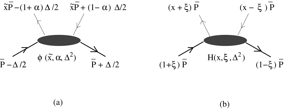
FIG. 2.:

FIG. 3.:

FIG. 4.:

FIG. 5.:

FIG. 6.:

FIG. 7.:

FIG. 8.: