UWThPh-2003-16
Neutrino Physics – Theory

Abstract

We discuss recent developments in neutrino physics and focus, in particular, on neutrino oscillations and matter effects of three light active neutrinos. Moreover, we discuss the difference between Dirac and Majorana neutrinos, neutrinoless $\beta\beta$-decay, absolute neutrino masses and electromagnetic moments. Basic mechanisms and a few models for neutrino masses and mixing are also presented.

1 Motivation

In recent years neutrino physics has gone through a spectacular development (for reviews see, for instance, [1, 2, 3, 4]). Data concerning solar and atmospheric neutrino deficits have been accumulated, these deficits have been established as neutrino physics phenomena and the Solar Standard Model [5] has been confirmed. The last steps of this exciting development were the results of the SNO [6] and KamLAND experiments [7]: The SNO experiment provided a model-independent proof of solar $\nu_{e}\to\nu_{\mu,\tau}$ transitions and the terrestrial disappearance of $\bar{\nu}_{e}$ reactor neutrinos in the KamLAND experiment has shown that the puzzle of the solar neutrino deficit is solved by neutrino oscillations [8]. This gives us confidence that the same is true for the atmospheric neutrino deficit as well. For information on the history of neutrino oscillations see [9, 10], for the recent experimental history see the contribution of G. Drexlin to these proceedings [4]. General reviews on neutrino physics can be found, for instance, in Refs. [11, 12, 13, 14].

These lecture notes are motivated by this development and aim at supplying the theoretical background for understanding and assessing it. In view of the importance of neutrino oscillations in this context, we will give a thorough discussion of vacuum neutrino oscillations and matter effects [15, 16] (see Section 2); the description of the latter is tailored for an understanding of the flavour transformation of solar neutrinos and effects in earth matter. Then, in Section 3, we will switch to the subject of the neutrino nature, which is a question of principal interest but has no impact on neutrino oscillations; we will work out the difference between Dirac and Majorana neutrinos and the basics of Majorana neutrino effects. Eventually, in Section 4, we will come to the least established field of neutrino physics: models for neutrino masses and mixing. In view of the huge number of models and textures, we cannot try to cover the field but rather discuss a small selection of basic mechanisms for generating neutrino masses and mixing. This selection will necessarily be biased due to personal interest and prejudices. A similar judgement has to be made concerning the literature quoted in these lecture notes; owing to the host of papers which have appeared in recent years only a small selection can be quoted here (for literature on neutrino experiments see Ref. [4]). Finally, we present conclusions in Section 5.

Abbreviations used in these lecture notes: CC = charged current, NC = neutral current, LBL = long baseline, SBL = short baseline, MSW = Mikheyev-Smirnov-Wolfenstein, LMA = large mixing angle, MM = magnetic moment, EDM = electric dipole moment, SM = Standard Model, SUSY = supersymmetry, GUT = Grand Unified Theory, VEV = vacuum expectation value.

2 Neutrino oscillations

2.1 Neutrino oscillations in vacuum

Here we give a simple and yet quite physical derivation of the neutrino oscillation formula. The first observation is that—as the NC interactions are flavour-blind—neutrino-flavour production and detection proceeds solely via CC interactions with the Hamiltonian density

$$\mathcal{H}_{cc}=\frac{g}{\sqrt{2}}W_{\rho}^{-}\sum_{\alpha=e,\mu,\tau}\bar{\ell}_{\alpha}\gamma^{\rho}\nu_{\alpha L}+\mathrm{H.c.}$$ (1)

The next observation is that flavour transitions are induced by neutrino mixing:

$$\nu_{\alpha L}=\sum_{j}U_{\alpha j}\nu_{jL}\,.$$ (2)

This relation means that the left-handed flavour fields are not identical with the left-handed components of the neutrino mass eigenfields $\nu_{j}$ corresponding to the mass $m_{j}$, but are related via a matrix $U$, which is determined by the neutrino mass term which will be discussed in Section 3. Here we simply assume the existence of the mixing matrix $U$ and the neutrino masses $m_{j}$.

We confine ourselves, apart from a few side remarks, to the following basic assumptions:

• There are three active neutrino flavours;

• The mixing matrix $U$ is a $3\times 3$ unitary matrix.

These assumptions are supported by the results of the neutrino oscillation experiments [4].

A crucial observation is that neutrino flavour is defined by the associated charged lepton in production and detection processes; there is no other physical way to define neutrino flavours. Looking at Eqs. (1) and (2), we find that, in a reasonable approximation, neutrino-flavour states are given by

$$|\nu_{\alpha}\rangle=\sum_{j=1}^{3}U_{\alpha j}^{*}|m_{j}\rangle\,,$$ (3)

where the mass eigenstates $|m_{j}\rangle$ fulfill the orthogonality condition

$$\langle m_{j}|m_{k}\rangle=\delta_{jk}\,.$$ (4)

The state (3) describes a neutrino with flavour $\alpha$ sitting at the position $x=0$. Every mass eigenstate propagates as a plane wave. If we have a stationary neutrino state with neutrino energy $E$, we derive from Eq. (3) the following form of the propagating state:

$$|\nu_{\alpha},x\rangle=\sum_{j=1}^{3}U_{\alpha j}^{*}e^{-i(Et-p_{j}x)}|m_{j}\rangle\,,$$ (5)

with neutrino momenta

$$p_{j}=\sqrt{E^{2}-m_{j}^{2}}\simeq E-\frac{m_{j}^{2}}{2E}\quad\mathrm{for}\quad E\gg m_{j}\,.$$ (6)

The latter inequality indicates the relativistic limit of massive neutrinos which is the relevant limit for all neutrino oscillation experiments.

Since the state $|\nu_{\alpha},x\rangle$ has flavour $\alpha$ at $x=0$, we compute the probability to find the flavour $\beta$ at $x=L$ by $|\langle\nu_{\beta}|\nu_{\alpha},L\rangle|^{2}$. With the explicit form (5) of $|\nu_{\alpha},x\rangle$ and with Eq. (6) we readily derive the standard formula of the neutrino transition or survival probability:

$$P_{\nu_{\alpha}\to\nu_{\beta}}(L/E)=\Bigg{|}\sum_{j=1}^{3}U_{\beta j}U_{\alpha j}^{*}e^{-im_{j}^{2}L/2E}\,\Bigg{|}^{2}.$$ (7)

It is easy to convince oneself that in the case of antineutrinos one simply has to make the replacement $U\to U^{*}$ in Eq. (7).

Looking at Eq. (7), we read off the following properties of $P_{\nu_{\alpha}\to\nu_{\beta}}$:

• It describes a violation of family lepton numbers;

• It is a function of mass-squared differences, e.g. of $m_{2}^{2}-m_{1}^{2}$ and $m_{3}^{2}-m_{1}^{2}$;

• It has an oscillatory behaviour in $L/E$;

• The relation $P_{\nu_{\alpha}\to\nu_{\beta}}=P_{\bar{\nu}_{\beta}\to\bar{\nu}_{\alpha}}$ is fulfilled as a reflection of CPT invariance;

• $P_{\nu_{\alpha}\to\nu_{\beta}}$ is invariant under the transformation $U_{\alpha j}\to e^{i\phi_{\alpha}}\,U_{\alpha j}\,e^{i\phi_{j}}$ with arbitrary phases $\phi_{\alpha}$, $\phi_{j}$.

Specializing Eq. (7) to 2-neutrino oscillations with flavours $\alpha\neq\beta$, one obtains the particularly simple formulas

$$U=\left(\begin{array}[]{rr}\cos\theta&\sin\theta\\ -\sin\theta&\cos\theta\end{array}\right),$$ (10)

$$P_{\nu_{\alpha}\to\nu_{\beta}}=\sin^{2}2\theta\times\frac{1}{2}\left(1-\cos\frac{\Delta m^{2}L}{2E}\right),$$ (11)

$$P_{\nu_{\alpha}\to\nu_{\beta}}=P_{\nu_{\beta}\to\nu_{\alpha}}\,,$$ (12)

$$P_{\nu_{\alpha}\to\nu_{\alpha}}=P_{\nu_{\beta}\to\nu_{\beta}}=1-P_{\nu_{\alpha}\to\nu_{\beta}}\,.$$ (13)

In Eq. (10) the rephasing invariance of $P_{\nu_{\alpha}\to\nu_{\beta}}$ has been used to reduce $U$ to a rotation matrix. For 2-neutrino oscillations the probabilities for neutrinos and antineutrinos are the same.

The oscillation phases in Eq. (7) have the form

$$\frac{\Delta m^{2}L}{2E}=2.53\times\left(\frac{\Delta m^{2}}{1\,\mathrm{eV}^{2}}\right)\times\left(\frac{1\,\mathrm{MeV}}{E}\right)\times\left(\frac{L}{1\,\mathrm{m}}\right),$$ (14)

where $\Delta m^{2}$ is one of the mass-squared differences. Alternatively, the oscillation phase is expressed by the oscillation length $L_{\mathrm{osc}}$ through

$$\frac{\Delta m^{2}L}{2E}\equiv 2\pi\,\frac{L}{L_{\mathrm{osc}}}\;\;\mathrm{with}\;\;L_{\mathrm{osc}}=2.48\,\mathrm{m}\,\times\left(\frac{E}{1\,\mathrm{MeV}}\right)\times\left(\frac{1\,\mathrm{eV}^{2}}{\Delta m^{2}}\right).$$ (15)

In a neutrino oscillation experiment, the sensitivity to $\Delta m^{2}$ is determined by the requirement that the phase (14) is of order one or not much smaller; this requirement depends on the characteristic ratio $L/E$ relevant for the experimental setup. By definition, SBL experiments are characterized by a sensitivity to $\Delta m^{2}\>\mbox{\raisebox{-3.0pt}{$\stackrel{{\scriptstyle\displaystyle>}}{{\sim}}$}}\>0.1$ eV², while terrestrial experiments with a sensitivity below 0.1 eV² are called LBL experiments. Note that using longer baselines or smaller energies moves the sensitivity to smaller mass-squared differences (see Eq. (14)).

No neutrino oscillation experiment has found a mass-squared difference $\Delta m^{2}\>\mbox{\raisebox{-3.0pt}{$\stackrel{{\scriptstyle\displaystyle>}}{{\sim}}$}}\>0.1$ eV², apart from the LSND experiment [17]. This experiment, however, has not not been confirmed by any other experiment and requires a forth neutrino which has to be sterile because the invisible Z width at LEP accommodates exactly the three active neutrinos. A sterile neutrino is defined as a neutral massive fermion which mixes with the active neutrinos, but has negligible couplings to the W and Z bosons. The result of the LSND experiment is at odds [18] with the combined data sets of either all other SBL experiments or the solar and atmospheric neutrino experiments, when interpreted in terms of 4-neutrino oscillations. See, however, Ref. [19], which shows that a 5-neutrino interpretation might reconcile the LSND result with the negative results of the other SBL experiments.

Let us discuss some concrete examples for the sensitivity to $\Delta m^{2}$. For reactor neutrinos the energy is about $E\sim 1$ MeV. Therefore, with $L\sim 1$ km, the sensitivity is $\Delta m^{2}\sim 10^{-3}$ eV²; this is the case of the CHOOZ [20] and Palo Verde [21] experiments. On the other hand, the KamLAND reactor experiment [7] with $L\sim 100$ km is sensitive down to $\Delta m^{2}\sim 10^{-5}$ eV². Experiments exploiting the source of atmospheric neutrinos with typical energies $E\sim 1$ GeV have as maximal baseline the diameter of the earth, i.e. $L\>\mbox{\raisebox{-3.0pt}{$\stackrel{{\scriptstyle\displaystyle<}}{{\sim}}$}}\>10^{4}$ km, from where the sensitivity $\Delta m^{2}\>\mbox{\raisebox{-3.0pt}{$\stackrel{{\scriptstyle\displaystyle>}}{{\sim}}$}}\>10^{-4}$ eV² follows. Solar neutrinos have a very long baseline of $L\simeq 150\times 10^{6}$ km and rather low energies of $E\sim 1\div 10$ MeV. Thus, in principle with solar neutrino experiments one can reach $\Delta m^{2}\sim 10^{-11}$ eV².

Quantum-mechanical aspects of neutrino oscillations:

Our phenomenological derivation of the oscillation probability (7) needs some quantum-mechanical support (for extensive reviews see Refs. [22, 23]). The points of our derivation which need justification are the following:

• We have employed stationary neutrino states, i.e., the plane waves have the same energy $E$ but different momenta $p_{j}$;

• The usage of plane waves for the neutrino mass eigenstates raises the question how this is compatible with the localization of neutrino source and detection in space.

In order to find limitations of the canonical oscillation probability we have to use a mathematical picture which is as close as possible to the actual situation of an experiment. Neutrinos are never directly observed; thus, for the description of neutrino oscillations it is required to consider the complete neutrino production–detection chain and to use only those quantities or particles which are really observed or manipulated in an experiment [24]. Consequently, we are lead to consider neutrino production and detection as a single big Feynman diagram where both the source and detector particle are described by wave packets which are localized in space, whereas the neutrinos are presented by inner lines of the big diagram; such models are called external wave packet models [23, 25] and the big diagram is treated in a field-theoretical way [26]. However, due to the macroscopic distance between source and detector the neutrinos are described as on-shell although they are on an inner line of the Feynman diagram [27].

We start with a consideration of the detector particle which is central to the first issue above [28, 29, 30]. In all experiments performed so far the detector particle is a bound state with energy $E_{D}$, either a nucleon in a nucleus or an electron in an atom. Such states are energy eigenstates. In addition, the detector bound state will experience thermal random movements with a whole spectrum of energies related to the temperature. However, there are no phase correlations between the different energy components of the thermal energy distribution which is, therefore, very well described by a density matrix which is diagonal in energy and the summation over this energy distribution is performed in the cross section corresponding to the big production–detection Feynman diagram [30, 31]. In other words, in the amplitude corresponding to the big diagram, we have a definite detector particle energy $E_{D}+\varepsilon^{D}_{\mathrm{thermal}}$, with an incoherent summation over the distribution of $\varepsilon^{D}_{\mathrm{thermal}}$ in the cross section.

Figure 1: The particles participating in the detector reaction at $\vec{x}_{D}$.

Concerning the $n_{D}$ final states in the detector reaction (see Fig. 1), we note that energy/momentum measurements are performed and that it is again summed incoherently over these energies $E^{\prime}_{Dk}$ in the cross section. Thus, looking at Fig. 1 we come to the conclusion that in the amplitude the neutrino energy $E$ is fixed and given by

$$E_{\nu}=\sum_{k}E^{\prime}_{Dk}-E_{D}-\varepsilon^{D}_{\mathrm{thermal}}\,.$$ (16)

Since the oscillation probability (7) is directly derived from the cross section, we come to following conclusion which has, in particular, been stressed by H. Lipkin [27, 28, 29, 30, 31]:

Neutrinos with the same energy $E$ but different momenta $p_{j}=\sqrt{E^{2}-m_{j}^{2}}$ are coherent.

Moreover, summation over the neutrino energies $E$ is effectively performed in the cross section, i.e., it is an incoherent summation and no wave packets are associated with neutrinos of definite mass.

Now we address the justification of the second point. Whereas it is necessary to assume localization in space of the neutrino source and detector wave functions, we stress that the final states in the source and detection reaction can be taken as plane waves; the reason is, as mentioned above, that the measurements performed with them are energy/momentum measurements and for calculating the cross section corresponding to the big Feynman diagram one has to sum incoherently, i.e. in the cross section, over the regions in phase space subject to kinematical restrictions according to the experiment. Denoting the detector particle wave function in phase space by $\tilde{\psi}_{D}(\vec{p}\,)$, a reasonable range for the width of this function is given by $\sigma_{D}\sim 10^{-3}\div 100$ MeV, where these limits are given for a detector particle bound in an atom or in a nucleus, respectively.

Figure 2: The wave function of the detector particle. The vertical line indicates the momentum difference $|p_{2}-p_{1}|$.

In Fig. 2 we have symbolically drawn a detector particle wave function. Looking at this 1-dimensional picture it is easy to find the condition for the existence of oscillations: Assuming for simplicity only two neutrinos, the neutrino mass eigenstates have the same energy $E$ but different momenta $p_{1}$, $p_{2}$ (6). Suppose that we fix the momenta of the final states of the detector process by $p^{\prime}_{Dk}$ ($k=1,\ldots,n_{D}$, see Fig. 1). By momentum conservation, the values of the detector wave function relevant for the amplitude of the complete production–detection cross section are given by $\tilde{\psi}_{D}\left(\sum_{k}\vec{p}\,^{\prime}_{Dk}-p_{j}\vec{\ell}\,\right)$ for each neutrino mass eigenstate, where $\vec{\ell}$ is a unit vector pointing from the source to the detector particle. Let us assume now that $\sum_{k}\vec{p}\,^{\prime}_{Dk}-p_{1}\vec{\ell}\simeq 0$. In order to obtain coherence between the neutrino states with mass $m_{1}$ and $m_{2}$, the momentum $p_{2}$ must not fulfill $|p_{2}-p_{1}|\gg\sigma_{D}$, because in that case we have $\tilde{\psi}_{D}\left(\sum_{k}\vec{p}\,^{\prime}_{Dk}-p_{2}\vec{\ell}\,\right)\simeq 0$, the two mass eigenstates do not interfere and there are no neutrino oscillations. Therefore, we are lead to the condition

$$|p_{2}-p_{1}|\simeq\Delta m^{2}/2E\>\mbox{\raisebox{-3.0pt}{$\stackrel{{\scriptstyle\displaystyle<}}{{\sim}}$}}\>\sigma_{D}$$ (17)

for neutrino oscillations—see Fig. 2. Denoting the width of the detector wave function in coordinate space by $\sigma_{xD}$, then with Heisenberg’s uncertainty relation $\sigma_{xD}\sim 1/2\sigma_{D}$ the condition (17) is rewritten as [27, 29, 32]

$$\sigma_{xD}\>\mbox{\raisebox{-3.0pt}{$\stackrel{{\scriptstyle\displaystyle<}}{{\sim}}$}}\>L_{\mathrm{osc}}/(4\pi)\,.$$ (18)

This condition is trivially fulfilled because $\sigma_{xD}$ is microscopic whereas $L_{\mathrm{osc}}$ is macroscopic! Similar considerations can be made for the neutrino source, with an additional condition taking into account that the source must be unstable [27, 29, 33]. Thus we can have confidence that the oscillation probability (7) holds for practical purposes.

The present discussion is certainly not the most general one but, as we believe, it is reasonably close to practical applications. It does not include the discussion of a coherence length, i.e. a maximal distance between source and detector until which coherence between different mass eigenstates is maintained. There is a vast literature on that point, see for instance Refs. [23, 25, 26, 34, 35] and citations therein. One detail can, however, be immediately deduced from our discussion: The better one determines experimentally the energies of all final states in the detection reaction, the better one determines the neutrino energy $E$. Since the coherence length is approximately obtained by $L_{\mathrm{osc}}\bar{E}/\Delta E$ [34], where $\bar{E}$ is the average neutrino energy and $\Delta E$ the neutrino energy spread, it is evident that by pure detector manipulations one can influence the coherence length and, in principle, by infinitely precise measurements of the energies of the final particles in the detector process, one could make it arbitrarily long [29, 34].

Some steps in the above investigation of the validity of the oscillation probability (7) have been criticized in the literature—see, for instance, Refs. [23, 25, 35]—and even the external wave packet model is not undisputed [35]. This suggests further investigations into the validity conditions of Eq. (7). However, since all attempts up to now to find limitations of (7) accessible to experiment were in vain, the standard formula for the probability of neutrino oscillations in vacuum seems to be very robust.

2.2 Matter effects

Matter effects [15, 16, 36] play a very important role in neutrino oscillations. Here we confine ourselves to the case of ordinary matter, which is non-relativistic, electrically neutral and without preferred spin orientation. It consists of electrons, protons and neutrons, i.e. fermions $f=e^{-}$, $p$, $n$. We denote the corresponding matter (number) densities by $N_{e}=N_{p}$ and $N_{n}$.

We want to present a simple heuristic and straightforward derivation of matter effects. First we notice that the vacuum oscillation probability (7) can be derived by using the Hamiltonian

$$H_{\nu}^{\mathrm{vac}}=\frac{1}{2E}U\hat{m}^{2}U^{\dagger}\,,$$ (19)

where $\hat{m}$ is the diagonal matrix of neutrino masses. In order to obtain the effective Hamiltonian in matter, we have to add to $H_{\nu}^{\mathrm{vac}}$ a term describing matter effects. With the above properties of ordinary matter we have the expectation values

$$\langle\bar{f}_{L}\gamma_{\mu}f_{L}\rangle_{\mathrm{matter}}=\frac{1}{2}N_{f}\delta_{\mu 0}\,.$$ (20)

Adding CC and NC contributions for neutrinos in the background of ordinary matter, the SM of electroweak interactions together with Eq. (20) provides us with the Hamiltonian density

$$\mathcal{H}^{\mathrm{mat}} = \frac{G_{F}}{\sqrt{2}}\sum_{\alpha=e,\mu,\tau}\nu_{\alpha}^{\dagger}(\mathbbm{1}-\gamma_{5})\nu_{\alpha}$$ (21)

$$\times\sum_{f}N_{f}(\delta_{\alpha f}+T_{3f_{L}}-2\sin^{2}\theta_{W}Q_{f})\,,$$

where $\delta_{\alpha f}$ comes from a Fierz transformation of the CC interaction, $\theta_{W}$ is the weak mixing angle, and $T_{3f_{L}}$ and $Q_{f}$ are the weak isospin and electric charge of the fermion $f$, respectively. Thus we arrive at the effective flavour Hamiltonian [15, 16]

$$H^{\mathrm{mat}}_{\nu}=\frac{1}{2E}U\hat{m}^{2}U^{\dagger}+\sqrt{2}\,G_{F}\,\mathrm{diag}\,\left(N_{e}-\frac{1}{2}N_{n},-\frac{1}{2}N_{n},-\frac{1}{2}N_{n}\right).$$ (22)

Then the evolution of a neutrino state undergoing oscillations and matter effects is calculated by solving

$$i\frac{da}{dx}=H_{\nu}^{\mathrm{mat}}\,a\quad\mathrm{with}\quad a=\left(\begin{array}[]{c}a_{e}\\[-2.84526pt] a_{\mu}\\[-2.84526pt] a_{\tau}\end{array}\right),$$ (23)

where $a_{e}$, $a_{\mu}$ and $a_{\tau}$ are the amplitudes of electron, muon and tau neutrino flavours.

For active neutrinos ($\nu_{\alpha}$ with $\alpha=e,\mu,\tau$) the neutron density $N_{n}$ can be dropped in the effective Hamiltonian, since it does not induce flavour transitions. Thus for active neutrinos only the electron density is relevant and there are no matter effects in 2-neutrino $\nu_{\mu}\to\nu_{\tau}$ transitions. If sterile neutrinos exist, $N_{n}$ does affect $\nu_{\alpha}\to\nu_{s}$ because sterile neutrinos do not experience matter effects, i.e., $N(\nu_{s})=0$ in $H^{\mathrm{mat}}_{\nu}$.

If we consider 2-neutrino oscillations, we obtain from Eq. (22) the well-known 2-flavour Hamiltonian by subtraction of an irrelevant diagonal matrix and by using the $2\times 2$ mixing matrix (10) [37]:

$$H_{\nu}^{\mathrm{mat}}=\frac{1}{4E}\left(\begin{array}[]{cc}A-\Delta m^{2}\cos 2\theta&\Delta m^{2}\sin 2\theta\\ \Delta m^{2}\sin 2\theta&-A+\Delta m^{2}\cos 2\theta\end{array}\right)$$ (24)

with

$$A=2\,\sqrt{2}\,G_{F}E\left[N(\nu_{\alpha})-N(\nu_{\beta})\right]$$ (25)

and $N(\nu_{e})=N_{e}-N_{n}/2$, $N(\nu_{\mu})=N(\nu_{\tau})=-N_{n}/2$, $N(\nu_{s})=0$. This equation shows once more what we have discussed above. From now on we do not discuss sterile neutrinos anymore in these lecture notes.

Performing all the analogous procedures for antineutrinos, we obtain $H^{\mathrm{mat}}_{\bar{\nu}}$ by making the replacements $U\to U^{*}$, matter term $\to$ $-$matter term in $H^{\mathrm{mat}}_{\nu}$ of Eq. (22).

In order to have an idea of the strength of matter effects, we estimate the “matter potential” $A$ for the two most important cases, the sun and the earth:

$$A=2\sqrt{2}G_{F}EN_{e}\simeq\left\{\begin{array}[]{l}\mbox{core of the sun:}\\ 1.5\times 10^{-5}\>\mbox{eV}^{2}\,\left(\frac{E}{1\;\mathrm{MeV}}\right),\\ \mbox{earth matter:}\\ 2.3\times 10^{-7}\>\mbox{eV}^{2}\>\left(\frac{\rho}{3\,\mathrm{g}\,\mathrm{cm}^{-3}}\right)\left(\frac{E}{1\;\mathrm{MeV}}\right).\end{array}\right.$$ (26)

The matter potential is the quantity which has to be compared with $\Delta m^{2}$ in order to estimate the influence of matter on neutrino oscillations.

In the evolution equation (23) the Hamiltonian is in general a function of the space coordinates through the electron density $N_{e}(x)$. Looking at the 2-neutrino Hamiltonian (24), a MSW resonance [16] occurs if there is a coordinate $x_{\mathrm{res}}$ such that

$$A(x_{\mathrm{res}})=\Delta m^{2}\cos 2\theta$$ (27)

holds. In this case, the probability of flavour transitions can be very big, in particular, if the neutrino goes adiabatically through the resonance point, as we shall see in the next subsection.

In the following, we will adopt—without loss of generality—the convention $\Delta m^{2}>0$ and $0^{\circ}\leq\theta\leq 90^{\circ}$ in the Hamiltonian (24). Therefore, the resonance condition is fulfilled for $\theta<45^{\circ}$ and a suitable electron density.

On the validity of the effective flavour Hamiltonian:

The heuristic derivation of matter effects resulting in the Hamiltonian (22) did not allow to see under which conditions Eqs. (22) and (23) hold. We now want to discuss a method which gives us some insight into the limitations of these equations. We follow Refs. [38, 39]. Suppose we have an incident wave propagating in $z$-direction which traverses a slab of matter of “infinitesimal” thickness $d$.

Figure 3: Scattering at a slab of matter of thickness $d$ of an incident wave propagating in $z$-direction

Then the incident wave undergoes multiple scattering at the scatterers $f$ with number density $N_{f}$ in the slab. According to Fig. 3 we sum over all scattered waves hitting a point on the $z$-axis at a distance $\ell$ from the slab and obtain

$$\begin{array}[]{l}\displaystyle N_{f}d\int_{0}^{\infty}\frac{e^{iE\sqrt{\rho^{2}+\ell^{2}}}}{\sqrt{\rho^{2}+\ell^{2}}}\mathcal{A}_{\nu_{\alpha}f}(E,\vartheta)\,2\pi\rho\,\mathrm{d}\rho=\\[11.38109pt] \displaystyle 2\pi N_{f}d\Bigg{\{}\frac{e^{iE\sqrt{\rho^{2}+\ell^{2}}}}{iE}\,\mathcal{A}_{\nu_{\alpha}f}(E,\vartheta)\Big{|}_{0}^{\infty}-\\[11.38109pt] \displaystyle\int_{0}^{\infty}\!\mathrm{d}\rho\,\frac{e^{iE\sqrt{\rho^{2}+\ell^{2}}}}{iE\ell\,[1+(\ell/\rho)^{2}]}\,\frac{\partial\mathcal{A}_{\nu_{\alpha}f}(E,\vartheta)}{\partial\vartheta}\Bigg{\}}.\end{array}$$ (28)

In this equation, $\mathcal{A}_{\nu_{\alpha}f}$ is the scattering amplitude. Eq. (28) can be considerably simplified. Firstly, it is reasonable to assume that in the term in the second line of this equation we can drop the limit $\rho\to\infty$ because that contribution averages out. Secondly, for $1/(E\ell)\ll 1$ and a smooth behaviour of the scattering amplitude, we can also drop the term in the third line of Eq. (28). Now we go one step further and consider a slab of finite thickness $D=kd$, where $d$ is “infinitesimal” whereas $k$ is a large integer. With the above-mentioned approximations we compute the phase of incident + transmitted wave through the finite slab as

$$\begin{array}[]{l}\lim_{k\to\infty}\left\{1+\frac{\displaystyle iED}{\displaystyle k}+\frac{\displaystyle 2\pi iN_{f}D\mathcal{A}_{\nu_{\alpha}f}(E,\vartheta=0)}{\displaystyle Ek}\right\}^{k}=\\[11.38109pt] \exp\left\{iED\left[1+2\pi N_{f}\mathcal{A}_{\nu_{\alpha}f}(E,\vartheta=0)/E^{2}\right]\right\}.\end{array}$$ (29)

The expression in the curly brackets of the first line of this equation, where the incident wave is represented by $1+iED/k\simeq\exp(iED/k)$, corresponds to the “infinitesimal” slab of thickness $d=D/k$ and $\ell=0$ (see Fig. 3); the power $k$ indicates that the wave propagates through $k$ such “infinitesimal” slabs. This consideration yields the well-known “index of refraction”

$$n(\nu_{\alpha})=1+\frac{2\pi}{E^{2}}\sum_{f}N_{f}\mathcal{A}_{\nu_{\alpha}f}(E,\vartheta=0)\,,$$ (30)

where only the forward-scattering amplitude, i.e. $\vartheta=0$ contributes. In $n(\nu_{\alpha})$ we have indicated that different types of scatterers can be distributed in the slab. Furthermore, the derivation of the “index of refraction” is evidently not specific to neutrino scattering.

$g_{V}$	$e^{-}$	$p$	$n$
$\nu_{e}$	$2\sin^{2}\theta_{w}+1/2$	$-2\sin^{2}\theta_{w}+1/2$	$-1/2$
$\nu_{\mu,\tau}$	$2\sin^{2}\theta_{w}-1/2$	$-2\sin^{2}\theta_{w}+1/2$	$-1/2$

Table 1: Vector coupling constants of the Hamiltonian density (31).

The connection with neutrino scattering is made by the Hamiltonian density

$$\mathcal{H}_{\nu_{\alpha}f}=\frac{G_{F}}{\sqrt{2}}\,\bar{\nu}_{\alpha}\gamma_{\rho}(\mathbbm{1}-\gamma_{5})\nu_{\alpha}\,\bar{f}\gamma^{\rho}\left(g_{V}^{(\alpha,f)}-g_{A}^{(\alpha,f)}\gamma_{5}\right)f\,.$$ (31)

The coupling constants $g_{V}^{(\alpha,f)}$ are found in Table 1. The axial-vector coupling constants do not contribute for ordinary matter (see Eq. (20)). As mentioned before, in the $\nu_{e}e^{-}$ scattering amplitude, there are CC + NC contributions, otherwise only NC interactions contribute. With the weak forward-scattering amplitude [39]

$$\mathcal{A}_{\nu_{\alpha}f}(E,\vartheta=0)=\frac{G_{F}E}{\sqrt{2}\pi}\,g_{V}^{(\alpha,f)}\,,$$ (32)

Eq. (29) and Table 1, we compute $2\pi\sum_{f}N_{f}\mathcal{A}_{\nu_{\alpha}f}(E,\vartheta=0)/E$ and obtain exactly the matter terms as in $\mathcal{H}_{\nu}^{\mathrm{mat}}$ in Eq. (22).

Now we use this second derivation of the matter potential as a means to check the validity of the Hamiltonian (22) [39]. We define two lengths: $d_{\mathrm{scatt}}$ is the average distance of scatterers in ordinary matter, $d_{\mathrm{var}}\sim N_{f}(x)/\big{|}\frac{dN_{f}(x)}{dx}\big{|}$ is the typical distance of matter density variations. Then we note the following conditions for the validity of Eqs. (22) and (23):

• $Ed_{\mathrm{scatt}}\gg 1\;\Rightarrow\;\lambda_{\nu}^{\mathrm{de\,Broglie}}\ll 2\pi d_{\mathrm{scatt}}$  ;

• $d_{\mathrm{scatt}}\ll d_{\mathrm{var}}$  ;

• $d_{\mathrm{scatt}}\ll L_{\mathrm{osc}}$  .

The 2nd and 3rd condition arise from the requirement of describing the neutrino state evolution by the differential equation (23). They are trivially fulfilled because $d_{\mathrm{scatt}}$ is microscopic, whereas $d_{\mathrm{var}}$ and $L_{\mathrm{osc}}$ are macroscopic. For instance for the sun we have $d_{\mathrm{var}}\sim 10^{4}$ km.

The first condition arises from the dropping of the term in the third line of Eq. (28). The quantity $\lambda_{\nu}^{\mathrm{de\,Broglie}}=2\pi/E$ is the de Broglie wave length of the neutrino. First we have to estimate $d_{\mathrm{scatt}}$. It is easy the convince oneself that to a very good approximation the electron density in matter is given by

$$N_{e}\simeq Y_{e}N_{A}(\rho/1\,g)\,,$$ (33)

where $Y_{e}$ is the number of electrons per nucleon, $\rho$ is the matter density in units of g/cm³ and $N_{A}\simeq 6.022\times 10^{23}$ is Avogadro’s constant. Let us check the first condition for the sun. According to the Solar Standard Model [5], in the solar core one has $\rho\simeq 150$ and $Y_{e}\simeq 2/3$, from where it follows that $N_{e}\simeq 100\,N_{A}$ cm^-3 and $d_{\mathrm{scatt}}=N_{e}^{-1/3}\simeq 0.25$ Å. Thus the first condition above is reformulated as $E\,d_{\mathrm{scatt}}\simeq 130\,E/(1\,\mathrm{MeV})\gg 1$. For solar neutrinos with $E\>\mbox{\raisebox{-3.0pt}{$\stackrel{{\scriptstyle\displaystyle>}}{{\sim}}$}}\>1$ MeV this condition is fulfilled. For earth matter this condition holds as well, because $d_{\mathrm{scatt}}$ is a little larger than in the solar core.

For other derivations of matter effects see Ref. [40] and references therein.

Survival probability for solar neutrinos:

We want to conclude this subsection by some general considerations concerning solar neutrinos within the framework of 2-neutrino oscillations. A neutrino produced in the solar core traverses first solar matter, then travels through vacuum to the neutrino detector on earth; during the night, the neutrino has to traverse, in addition, some stretch of earth matter. We denote by $P^{S}_{e1,2}$ the probability for $|\nu_{e}\rangle\to|\nu_{1,2}\rangle$ in the sun. Furthermore, the probability of $|\nu_{1,2}\rangle\to|\nu_{e}\rangle$ transitions in earth matter is called $P^{E}_{1,2e}$. Note that with the $2\times 2$ mixing matrix $U$ of Eq. (10) during the day we have

$$P^{E}_{1e}=\cos^{2}\theta\quad\mathrm{and}\quad P^{E}_{2e}=\sin^{2}\theta\,,$$ (34)

where $\theta$ is the solar neutrino mixing angle. Then the survival probability of solar electron neutrinos is written as [41]

$$P_{\nu_{e}\to\nu_{e}} = P^{S}_{e1}P^{E}_{1e}+P^{S}_{e2}P^{E}_{2e}+$$ (35)

$$2\,\sqrt{P^{S}_{e1}P^{E}_{1e}P^{S}_{e2}P^{E}_{2e}}\cos(\delta_{m}+\Delta m^{2}L_{\mathrm{vac}}/2E)\,.$$

In this formula, $L_{\mathrm{vac}}\simeq 150\times 10^{6}$ km is the distance between the surface of the sun and the surface of the earth along the neutrino trajectory, i.e. $\Delta m^{2}L_{\mathrm{vac}}/2E$ is the phase the neutrino acquires in vacuum. The phase acquired in matter is denoted by $\delta_{m}$.

Eq. (35) is completely general. One obvious questions arises: Under which conditions can the interference term in $P_{\nu_{e}\to\nu_{e}}$ be dropped? To investigate this point one can make a rough estimate. The size of the neutrino production region is approximately the diameter $\ell_{\mathrm{core}}$ of the solar core. Therefore, for $\Delta m^{2}\ell_{\mathrm{core}}/2E\>\mbox{\raisebox{-3.0pt}{$\stackrel{{\scriptstyle\displaystyle>}}{{\sim}}$}}\>2\pi$ with $\ell_{\mathrm{core}}\sim 10^{5}$ km, we obtain the condition

$$\Delta m^{2}/E>10^{-14}\;\mathrm{eV}\quad\Rightarrow\quad\left\langle\cos(\delta_{m}+\Delta m^{2}L_{\mathrm{vac}}/2E)\right\rangle_{\mathrm{core}}=0\,.$$ (36)

This argument is not completely correct because of the matter effects, but numerical calculations give the same result [41]. On the other hand, experiments cannot measure the neutrino energy $E$ with infinite precision and energy averaging in the vacuum phase occurs. If $(\Delta m^{2}L/2E)(\delta E/E)\>\mbox{\raisebox{-3.0pt}{$\stackrel{{\scriptstyle\displaystyle>}}{{\sim}}$}}\>2\pi$, where $\delta E$ is the uncertainty in the measurement of $E$, with an optimistic assumption of $\delta E/E\sim 10^{-2}$ we again arrive at Eq. (36).

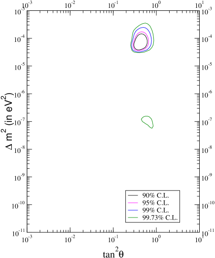
Figure 4: Allowed regions in the $\tan^{2}\theta$–$\Delta m^{2}$ plane for the 2-neutrino oscillation solutions of the solar neutrino deficit. The upper region represents the LMA MSW solution, the lower one the LOW solution. This plot showing the status after the SNO results but before the KamLAND result has been taken from Ref. [42].

For the LMA MSW oscillation solution of the solar neutrino puzzle with $\Delta m^{2}\sim 10^{-5}$ eV², condition (36) is very well fulfilled, and for the LOW solution—named after its “low” mass-squared difference of $\Delta m^{2}\sim 10^{-7}$ eV²—this condition is still fulfilled [41]. For the allowed regions in the $\tan^{2}\theta$–$\Delta m^{2}$ plane of these solutions see Fig. 4. Note that this figure is relevant for the situation after the SNO results but before the KamLAND result which has ruled out the LOW region in the plot. For the recent history of solar neutrino oscillations see Ref. [4]. For the LMA MSW solution the resonance condition (27) plays an important role, as we will see in the next subsection.

2.3 Adiabatic neutrino evolution in matter

Now we want to discuss adiabatic neutrino evolution in matter. We focus on solar neutrinos and confine ourselves to 2-neutrino flavours. Solutions of the 2-neutrino differential equation

$$i\frac{d}{dx}\left(\begin{array}[]{c}a_{e}\\ a_{x}\end{array}\right)=H_{\nu}^{\mathrm{mat}}\left(\begin{array}[]{c}a_{e}\\ a_{x}\end{array}\right)$$ (37)

can be found by numerical integration and, for instance, the plots of allowed $\tan^{2}\theta$–$\Delta m^{2}$ regions of solar neutrino oscillations like Fig. 4 are usually obtained via such numerical solutions, taking into account averaging over the solar neutrino production region. Eq. (37) refers to $\nu_{e}\to\nu_{x}$ transitions. In the next subsection, in the context of three neutrino flavours, we will discuss to which $\nu_{\mu}$–$\nu_{\tau}$ flavour combination the amplitude $a_{x}$ refers. The Hamiltonian $H_{\nu}^{\mathrm{mat}}$ is given by Eq. (24).

In general, solutions of Eq. (37) will be non-adiabatic. However, since the result of the KamLAND experiment we know that the solar neutrino puzzle is solved by neutrino oscillations corresponding to the LMW MSW solution; we will argue here that this solution behaves very well adiabatically.

For the consideration of adiabaticity (see, for instance, Ref. [43]) we need the eigenvectors of $H^{\mathrm{mat}}_{\nu}$, which are defined $\forall\,x$ by

$$H^{\mathrm{mat}}_{\nu}(x)\psi_{mj}(x)=E_{j}(x)\psi_{mj}(x)\,,$$ (38)

where

$$\psi_{m1}=\left(\begin{array}[]{r}\cos\theta_{m}\\ -\sin\theta_{m}\end{array}\right),\;\psi_{m2}=\left(\begin{array}[]{r}\sin\theta_{m}\\ \cos\theta_{m}\end{array}\right).$$ (39)

In the 2-flavour case discussed here and with the real Hamiltonian (24), one parameter, the matter angle $\theta_{m}$, is sufficient to parameterize the two eigenvectors (39). With Eq. (24) the matter angle is expressed as

$$\tan 2\theta_{m}(x)=\frac{\tan 2\theta}{\displaystyle 1-\frac{A(x)}{\Delta m^{2}\cos 2\theta}}\quad\mathrm{with}\quad A(x)=2\sqrt{2}EN_{e}(x)\,.$$ (40)

Note that for $A\to 0$, i.e. negligible matter effects, we obtain $\theta_{m}\to\theta$, i.e., the matter angle becomes identical with the (vacuum) mixing angle of $U$ of Eq. (10).

The full solution of the differential equation (37) can be written as

$$\psi(x)=\sum_{j=1,2}a_{j}(x)\psi_{mj}(x)e^{-i\varphi_{j}(x)}\quad\mathrm{with}\quad\varphi_{j}=\int_{x_{0}}^{x}dx^{\prime}E_{j}(x^{\prime})\,.$$ (41)

Having in mind solar neutrinos, we identify $\Delta m^{2}$ with the solar mass-squared difference and use the initial condition that at $x_{0}$ a $\nu_{e}$ is produced. This leads to

$$\psi(x_{0})=\left(\begin{array}[]{c}1\\ 0\end{array}\right)\;\Rightarrow\left\{\begin{array}[]{c}a_{1}(x_{0})=\cos\theta_{m}(x_{0})\,,\\ a_{2}(x_{0})=\sin\theta_{m}(x_{0})\,.\end{array}\right.$$ (42)

Eq. (41) is completely general. A solution is called adiabatic if the following condition is fulfilled.

$$\mathrm{Adiabaticity:}\quad a_{1,2}(x)\simeq\mathrm{constant}.$$ (43)

In that case we have $a_{1,2}(x)\simeq a_{1,2}(x_{0})$ and with Eq. (42) we obtain

$$P^{S}_{e1}=\cos^{2}\theta_{m}(x_{0})\,,\quad P^{S}_{e2}=\sin^{2}\theta_{m}(x_{0})\,.$$ (44)

Using now that the interference term in Eq. (35) can be dropped for the LMA MSW solution and taking into account Eq. (34), we compute

$$P_{\nu_{e}\to\nu_{e}} = \cos^{2}\theta_{m}(x_{0})\cos^{2}\theta+\sin^{2}\theta_{m}(x_{0})\sin^{2}\theta$$ (45)

$$= \frac{1}{2}\Big{(}1+\cos 2\theta_{m}(x_{0})\cos 2\theta\Big{)}.$$

This is the well-known survival probability for adiabatic neutrino evolution from matter to vacuum. Since we used Eq. (34), it does not include earth matter effects.

Let us now consider effects of non-adiabaticity. Plugging the full solution (41) into Eq. (37), we derive an equation for the coefficients $a_{1,2}$:

$$\frac{\mathrm{d}}{\mathrm{d}x}\left(\begin{array}[]{c}a_{1}\\ a_{2}\end{array}\right)=\left(\begin{array}[]{cc}0&-\frac{\mathrm{d}\theta_{m}}{\mathrm{d}x}e^{i\varphi}\\ \frac{\mathrm{d}\theta_{m}}{\mathrm{d}x}e^{-i\varphi}&0\end{array}\right)\left(\begin{array}[]{c}a_{1}\\ a_{2}\end{array}\right),$$ (46)

where we have used the definition

$$\varphi=\varphi_{1}-\varphi_{2}=\int_{x_{0}}^{x}dx^{\prime}\Delta E\quad\mathrm{with}\quad\Delta E=E_{1}-E_{2}\,.$$ (47)

With the Hamiltonian (24) we calculate

$$\Delta E=\frac{1}{2E}\,\sqrt{(A-\Delta m^{2}\cos 2\theta)^{2}+(\Delta m^{2}\sin 2\theta)^{2}}\,.$$ (48)

If along the neutrino trajectory the phase factor $\exp(i\varphi)$ in Eq. (46) oscillates very often while the change in $\theta_{m}$ is of order one, then $\dot{a}_{1,2}$ will be approximately zero. This suggest the introduction of the “adiabaticity parameter” [44, 45, 46]

$$\gamma(x)\equiv\Delta E/2|\dot{\theta}_{m}|\,.$$ (49)

Therefore, we conclude

$$\mathrm{Adiabaticity}\;\Leftrightarrow\;\gamma\gg 1$$ (50)

along the neutrino trajectory. In vacuum, $\gamma=\infty$, in agreement with $a_{1,2}$ being exactly constant. Non-adiabaticity is quantified by the probability $P_{c}$ for crossing from $\psi_{m1}$ to $\psi_{m2}$. It corrects Eq. (45) to [45]

$$P_{\nu_{e}\to\nu_{e}}=\frac{1}{2}+\left(\frac{1}{2}-P_{c}\right)\cos 2\theta_{m}(x_{0})\cos 2\theta\,.$$ (51)

Again, as in Eq. (45), this form of the survival probability holds where Eq. (36) is valid. The adiabaticity parameter $\gamma$ can be used to find a mathematically exact upper bound on $P_{c}$ [12].

Reverting to solar neutrinos, we use that the electron density in the sun fulfills

$$N_{e}(x)\propto\exp{(-x/r_{0})}\,,$$ (52)

except for the inner part of the core and toward the edge [5], with $r_{0}\simeq R/10.54\simeq 6.6\times 10^{4}\>\mathrm{km}\leftrightarrow 3.3\times 10^{20}\>\mathrm{MeV}^{-1}$; $R$ is the solar radius. We want to estimate $\gamma$ for the case that the neutrino goes through a resonance (27) in a region where the exponential form of the electron density provides a good approximation. Then adiabaticity will be rather well fulfilled if it is fulfilled at the resonance point [44, 45, 46, 47]. There, $\gamma$ is given by

$$\gamma_{\mathrm{res}}=\frac{\Delta m^{2}\sin^{2}2\theta}{2E\cos 2\theta(|\dot{A}|/A)_{\mathrm{res}}}\simeq\frac{\Delta m^{2}r_{0}}{2E}\times\cos 2\theta\tan^{2}2\theta\,.$$ (53)

For large $\theta$ and close to the solar edge this estimate for adiabaticity is not correct (see Ref. [48]).

Now we turn to the characteristics of the LMA MSW solar neutrino solution with $\Delta m^{2}\sim 7\times 10^{-5}$ eV² and $\theta\sim 34^{\circ}$ [1, 2]. Writing the oscillation length (15) as

$$L_{\mathrm{osc}}=35\>\mbox{km}\left(\frac{7\times 10^{-5}\>\mathrm{eV}^{2}}{\Delta m^{2}}\right)\left(\frac{E}{1\>\mathrm{MeV}}\right),$$ (54)

it is evident that in this case the flavour transition occurs inside the sun. Furthermore, with Eq. (53) we estimate $\gamma_{\mathrm{res}}\sim 10^{3}$ and the LMA MSW oscillation solution is clearly in the adiabatic regime. Other interesting features of the LMA MSW solution emerge by considering the limit of increasing neutrino energy:

$$E\uparrow\;\Rightarrow\left\{\begin{array}[]{l}x_{\mathrm{res}}\>\mbox{moves outward},\\ \theta_{m}(x_{0})\to\pi/2\,,\\ P^{S}_{e1}\to 0,\;P^{S}_{e2}\to 1\,,\\ P_{\nu_{e}\to\nu_{e}}\to\frac{1}{2}\left(1-\cos 2\theta\right)=\sin^{2}\theta\,.\end{array}\right.$$ (55)

The first line follows from Eq. (27) and the fact that $N_{e}(x)$ is monotonically decreasing from the center to the edge of the sun. The other properties in Eq. (55) are read off from Eqs. (40), (44) and (45), respectively. We remind the reader that the latter limit does not include earth matter effects, therefore, it holds only during the day, just as Eq. (45). Note that from $P^{S}_{e2}\to 1$ we conclude that for large enough solar neutrino energies we have a transition

$$|\nu_{e}\rangle_{\mathrm{core}}\to|\nu_{2}\rangle_{\mathrm{edge}}\,.$$ (56)

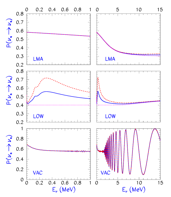
Figure 5: Comparison of the survival probabilities for LMA MSW, LOW and vacuum solar neutrino oscillations for an electron neutrino created in the center of the sun. The figure has been taken from Ref. [49]. The dotted lines refer to the daytime, whereas the dashed line includes $\nu_{e}$ regeneration during the night, when earth matter is effective. The full line refers to the average survival probability.

In Fig. 5 the solar $\nu_{e}$ survival probability is depicted. For historical reasons, $P_{\nu_{e}\to\nu_{e}}$ is depicted not only for the LMA MSW, but also the LOW and vacuum oscillation probabilities which are both ruled out now. The dotted lines refer to daytime, i.e., when earth matter has no effect. The LMA MSW best fit of Ref. [49] is given by $\Delta m^{2}=5.0\times 10^{-5}$ eV² and $\tan^{2}\theta=0.42$ (after the SNO but before the KamLAND result). Let us now make a small numerical exercise. From the best fit we get $\sin^{2}\theta=0.30$, which should give $P_{\nu_{e}\to\nu_{e}}$ for large $E$. Indeed, looking at the right end of the dotted curve in the right LMA panel where $E=15$ MeV, we find excellent agreement. We see that neutrino energies around 10 MeV are already “large” in the sense of the limit (55). On the other hand, let us take the limit $E\to 0$. In that limit the neutrino does not go through a resonance because Eq. (27) cannot be fulfilled. Therefore, because of the short oscillation length (54), we expect an averaged survival probability $P_{\nu_{e}\to\nu_{e}}=1-\frac{1}{2}\sin^{2}2\theta$ (see Eqs. (11) and (13)). Numerically, we obtain $1-\frac{1}{2}\sin^{2}2\theta=0.58$, in excellent agreement with the left ends of the LMA panels. We have thus demonstrated here that qualitatively the LMA MSW solution can be quite easily understood.

We have not discussed earth matter effects here. Looking at the right LMA panel in Fig. 5, we see that, at energies $E\>\mbox{\raisebox{-3.0pt}{$\stackrel{{\scriptstyle\displaystyle>}}{{\sim}}$}}\>10$ MeV, during the night when earth matter effects are operative the $\nu_{e}$ survival probability is a little larger than during the day. This introduces a small day–night asymmetry due to $\nu_{e}$ regeneration in earth matter. For a qualitative understanding of this effect see Ref. [50].

Small $\Delta m^{2}$ and the limit of strong non-adiabaticity:

Here we want to discuss the question How do solar neutrinos approach vacuum oscillations in the limit of small $\Delta m^{2}$ ? This is a non-trivial question because for small $\Delta m^{2}$ there is always a point where the resonance condition (27) holds. Of course, this is a purely academic question since we know that solar neutrinos follow the LMA MSW solution for which the resonance does play a prominent role. It is, however, an interesting question from the point of view of neutrino evolution in matter in general.

When we speak of vacuum oscillations of solar neutrinos we mean mass-squared differences of the order of $\Delta m^{2}\sim 10^{-10}$ eV² for which the oscillation length is of the order of the distance between sun and earth. From the resonance condition (27) we read off that in this case the resonance is very close to the solar edge (in this context, see $N_{e}(x)$ in Ref. [5]). From Eq. (40) it follows that $\theta_{m}(x_{0})=\pi/2$ and that $\dot{\theta}_{m}=0$ holds until very close to the resonance. It is easy to check that the width of the resonance, i.e. the distance where the change in $A(x)$ is of the order of $\Delta m^{2}\cos 2\theta$, is roughly $r_{0}$, where the electron density $N(x)$ behaves like Eq. (52). Close to the edge of the sun the electron density drops steeper and the resonance width is smaller. Then one can check that while the neutrino crosses the resonance and also between the resonance and the solar edge one can approximate the phase $\varphi$ of Eq. (47) by a constant, which can be taken as its value at the solar edge. This is just the opposite of adiabaticity—see the discussion after Eq. (46). For constant $\varphi$ the solution of Eq. (46) is given by

$$\left(\begin{array}[]{c}a_{1}(x)\\ a_{2}(x)\end{array}\right)=\left(\begin{array}[]{cc}\cos\Delta\theta_{m}&-e^{i\varphi}\sin\Delta\theta_{m}\\ e^{-i\varphi}\sin\Delta\theta_{m}&\cos\Delta\theta_{m}\end{array}\right)\left(\begin{array}[]{c}a_{1}(x_{0})\\ a_{2}(x_{0})\end{array}\right)$$ (57)

with $\Delta\theta_{m}\equiv\theta_{m}(x)-\theta_{m}(x_{0})$. In the case under discussion, the solution (57) is valid from just before the resonance till the solar edge and in the beginning of the vacuum. The initial conditions are $\theta_{m}(x_{0})=\pi/2$ and $a_{1}(x_{0})=0$, $a_{2}(x_{0})=1$ . Then with Eq. (57), at the solar edge, we get $a_{1}=e^{i\varphi}\cos\theta$, $a_{2}=\sin\theta$. Plugging this result into the full solution (41), we find what we expect: After the resonance, i.e. from the the solar edge onward, neutrinos perform ordinary vacuum oscillations; even the matter effects accumulated in the phases $\varphi_{1,2}$ cancel. Inside the sun before the resonance, oscillations are completely suppressed because of the matter effects, due to $A\gg\Delta m^{2}|\cos 2\theta|$. For further details see Ref. [48].

2.4 3-neutrino oscillations and the mixing matrix

Neutrino mass spectra:

Up to now all possible neutrino mass spectra, i.e. hierarchical, inverted hierarchy, degenerate, etc., are compatible with present data. By convention we have stipulated $m_{1}<m_{2}$ or $\Delta m^{2}_{21}\equiv\Delta m^{2}_{\odot}>0$, where we have used the definition $\Delta m^{2}_{jk}=m_{j}^{2}-m_{k}^{2}$. Thus there are two possibilities for $m_{3}$ according to $\Delta m^{2}_{31}\,\raisebox{-2.84526pt}{$\stackrel{{\scriptstyle>}}{{\scriptstyle<}}$}\,0$. Correspondingly, there are the two types of spectra depicted in Fig. 6:

Figure 6: The normal and the inverted 3-neutrino mass spectrum.

The “normal” and the “inverted” spectrum [51]. The hierarchical spectrum emerges in the limit $m_{1}\to 0$ of the normal spectrum, whereas the “inverted” hierarchy is obtained from the inverted spectrum with $m_{3}\to 0$.

In the 3-neutrino case the atmospheric mass-squared difference is not uniquely defined. If by convention we use for $\Delta m^{2}_{\mathrm{atm}}$ the largest possible mass-squared difference, then for the normal spectrum we obtain $\Delta m^{2}_{\mathrm{atm}}=\Delta m^{2}_{31}$ and for the inverted case we have $\Delta m^{2}_{\mathrm{atm}}=\Delta m^{2}_{23}$.

The mixing matrix:

The most popular parameterization of the neutrino mixing matrix is given by [52]

$$U=U_{23}U_{13}U_{12}$$ (58)

with

$$U_{23} = \left(\begin{array}[]{ccc}1&0&0\\ 0&c_{23}&s_{23}\\ 0&-s_{23}&c_{23}\end{array}\right),$$ (62)

$$U_{13} = \left(\begin{array}[]{ccc}c_{13}&0&s_{13}e^{-i\delta}\\ 0&1&0\\ -s_{13}e^{i\delta}&0&c_{13}\end{array}\right),$$ (66)

$$U_{12} = \left(\begin{array}[]{ccc}c_{12}&s_{12}&0\\ -s_{12}&c_{12}&0\\ 0&0&1\end{array}\right).$$ (70)

The mixing angle $\theta_{12}\equiv\theta_{\odot}$ is probed in the solar neutrino experiments and in the KamLAND experiment. The mixing angle $\theta_{23}\equiv\theta_{\mathrm{atm}}$ is the relevant angle in atmospheric and LBL neutrino oscillation experiments. Up to now now effects of a non-zero angle $\theta_{13}$ have not been seen.

3-neutrino oscillations:

The principle of 3-neutrino oscillations is a consequence of $\Delta m^{2}_{\odot}\ll\Delta m^{2}_{\mathrm{atm}}$ and can be summarized in the following way.

$\Delta m^{2}_{\mathrm{atm}}L/(2E)\sim 1$ $\Rightarrow$ $\Delta m^{2}_{\odot}L/(2E)\ll 1$ Solar $\nu$ oscillations frozen in atm./LBL $\nu$ osc.!

$\Delta m^{2}_{\odot}L/(2E)\sim 1$ $\Rightarrow$ $\Delta m^{2}_{\mathrm{atm}}L/(2E)\gg 1$ Atm. $\nu$ oscillations averaged in solar $\nu$ osc.!

Since, at present, $\theta_{13}=0$ is compatible with all available neutrino data, only an upper bound on this angle can be extracted. The two most important results in this context are:

• The non-observation of $\nu_{e}$ disappearance in the CHOOZ [20] and Palo Verde [21] experiments;

• The non-observation of atmospheric $\nu_{e}$ or $\bar{\nu}_{e}$ disappearance [4].

Also solar neutrino data have an effect on $\theta_{13}$, although small, because in the 3-neutrino case the solar survival probability is given by

$$P_{\nu_{e}\to\nu_{e}}^{\odot}\simeq c_{13}^{4}\,P^{(2)}_{\nu_{e}\to\nu_{e}}(\Delta m^{2}_{21},\theta_{12},c_{13}^{2}N_{e})+s_{13}^{4}\,,$$ (71)

where $P^{(2)}_{\nu_{e}\to\nu_{e}}$ is a 2-neutrino probability, calculated with the electron density $c_{13}^{2}N_{e}$ instead of $N_{e}$. The result of fits to the neutrino data is [53]

$$\sin^{2}\theta_{13}<0.05\;\mathrm{at}\;3\sigma\,.$$ (72)

As evident from the parameterization (58), CP violation disappears from neutrino oscillations for $\theta_{13}\to 0$.

In atmospheric neutrino experiments the mixing parameter which is extracted is

$$\sin^{2}2\theta_{23}\simeq 4|U_{\mu 3}|^{2}(1-|U_{\mu 3}|^{2})\,,$$ (73)

where we have taken into account the smallness of $\theta_{13}$. The Super-Kamiokande experiment finds a result [54] compatible with maximal mixing:

$$\sin^{2}2\theta_{23}>0.92\;\mathrm{at}\;\mbox{90\% CL.}$$ (74)

This leads to $0.60<|U_{\mu 3}|<0.80$. Note that $\theta_{23}=45^{\circ}$ corresponds to $|U_{\mu 3}|=1/\sqrt{2}\simeq 0.707$.

Now we want to discuss the states into which solar and atmospheric neutrinos are transformed. In the limit $\theta_{13}\to 0$ or $U_{13}\to\mathbbm{1}$ this discussion is most transparent. In that limit, in terms of neutrino states, atmospheric neutrino oscillations are given by $|\nu_{\mu}\rangle\to|\nu_{\tau}\rangle$, $|\bar{\nu}_{\mu}\rangle\to|\bar{\nu}_{\tau}\rangle$, while $\nu_{e}$ and $\bar{\nu}_{e}$ do not oscillate because their oscillation amplitude is given by $\sin^{2}2\theta_{13}$. In the context of Eq. (37) the question was raised to which neutrino state the amplitude $a_{x}$ belongs. For the evolution of neutrino states in the sun, the mass eigenstate $|\nu_{3}\rangle=s_{23}|\nu_{\mu}\rangle+c_{23}|\nu_{\tau}\rangle$ is an approximate eigenstate of $H_{\nu}^{\mathrm{mat}}$ because $|\Delta m^{2}_{31}|\gg A$ (see Eq. (26)). Therefore, the initial state $|\nu_{e}\rangle_{\odot}$ must transform with probability $P_{\nu_{e}\to\nu_{e}}^{\odot}$ into the state orthogonal to $|\nu_{3}\rangle$, from where it follows that (without earth regeneration effects)

$$|\nu_{e}\rangle_{\odot}\to-c_{23}|\nu_{\mu}\rangle+s_{23}|\nu_{\tau}\rangle\,.$$ (75)

Note that Eq. (71) has been derived by using the approximate eigenvector property of $|\nu_{3}\rangle$, but corrections for non-zero $\theta_{13}$ have been made.

The primary goal of LBL neutrino oscillation experiments is the check of atmospheric neutrino results, observation of $\nu_{\tau}$ appearance and the oscillatory behaviour in $L/E$ [4]. The demonstration of the latter property would give us the final proof that atmospheric $\nu_{\mu}$ and $\bar{\nu}_{\mu}$ disappearance is really an effect of oscillations. Let us make a list what we would wish to gain from LBL (K2K with $L=250$ km, MINOS and CERN-Gran Sasso with $L=730$ km) and very LBL experiments:

• Precision measurements of $\Delta m^{2}_{\mathrm{atm}}$ and $\theta_{23}$;

• Measurement of $\theta_{13}$;

• Verification of matter effects and distinction between normal and inverted mass spectra;

• Effects of $\Delta m^{2}_{\odot}$ and CP violation.

We want to stress the difficulty of measuring CP violation in neutrino oscillations: Such an effect is only present if $\sin\theta_{13}\neq 0$ and if the experiment is sensitive to both mass-squared differences, atmospheric and solar, thus the measurements must be accurate to such a degree that they invalidate the principle of 3-neutrino oscillations mentioned in the beginning of this subsection. Furthermore, the earth matter background in (very) LBL experiments fakes effects of CP violation which have to be separated from true CP violation.

Very LBL experiments are planned with super neutrino beams [55] and neutrino factories [56]. Super neutrino beams are conventional but very-high-intensity and low-energy ($E\sim 1$ GeV) beams, with the neutrino detector slightly off the beam axis; the JHF–Kamioka Neutrino Project with $L=295$ km is scheduled to start in 2007 [55]. Neutrino factories are muon storage rings with straight sections from where well-defined neutrino beams from muon decay emerge. According to the list above, measuring $\nu_{e}\to\nu_{\mu}$ and $\bar{\nu}_{e}\to\bar{\nu}_{\mu}$ transitions is of particular interest; note that $\theta_{13}$ is the only angle in the neutrino mixing matrix which has not been measured up to now. One can easily convince oneself that this task is tackled by measuring the so-called “wrong-sign” muons; e.g., $\mu^{-}_{\mathrm{storage}}\to\mu^{+}_{\mathrm{detector}}$ corresponds to $\bar{\nu}_{e}\to\bar{\nu}_{\mu}$. Neutrino factories are under investigation. Optimization conditions for running such a machine are considered in the ranges $20\>\mbox{\raisebox{-3.0pt}{$\stackrel{{\scriptstyle\displaystyle<}}{{\sim}}$}}\>E_{\mu}\>\mbox{\raisebox{-3.0pt}{$\stackrel{{\scriptstyle\displaystyle<}}{{\sim}}$}}\>50$ GeV and $L\>\mbox{\raisebox{-3.0pt}{$\stackrel{{\scriptstyle\displaystyle>}}{{\sim}}$}}\>3000$ km. For further references see, e.g., [57, 58, 59, 60] and citations therein.

3 Dirac versus Majorana neutrinos

In this section we focus, in particular, on Majorana neutrinos. Apart from the vanishing electric charge, also most of the popular extensions of the SM suggest that neutrinos have Majorana nature. Majorana particles have several interesting features, which make them quite different from Dirac particles. Unfortunately, in practice, due to the smallness of the masses of the light neutrinos, it is quite difficult to distinguish between both natures: Neutrinoless $\beta\beta$-decay seems to be the only promising road so far. In any case, neutrino oscillations do not distinguish between Dirac and Majorana neutrinos, since there only the states with negative helicity enter, where this distinction is irrelevant. Though family lepton numbers must be violated for transitions $\nu_{\alpha}\to\nu_{\beta}$, the total lepton number remains conserved.

3.1 Free fields

With two independent chiral 4-spinor fields $\psi_{L,R}$ one can construct the usual Lorentz-invariant bilinear for Dirac fields which is called mass term:

$$\mbox{Dirac:}\quad-m\left(\bar{\psi}_{R}\psi_{L}+\mbox{H.c.}\right)=-m\bar{\psi}\psi\quad\mbox{with}\quad\psi=\psi_{L}+\psi_{R}\,.$$ (76)

With only one chiral 4-spinor $\psi_{L}$ one obtains nevertheless a Lorentz-invariant bilinear with the help of the charge-conjugation matrix $C$:

$$\mbox{Majorana:}\;\>\frac{1}{2}m\psi_{L}^{T}C^{-1}\psi_{L}+\mbox{H.c.}=-\frac{1}{2}m\bar{\psi}\psi\;\mbox{with}\;\psi=\psi_{L}+(\psi_{L})^{c}.$$ (77)

Note that from $\psi_{L}$ one obtains a right-handed field with the charge-conjugation operation $(\psi_{L})^{c}\equiv C\gamma_{0}^{T}\psi_{L}^{*}$; in contrast to the Dirac case, this right-handed field is not independent of the left-handed field.

The equation for free Dirac or Majorana fields in terms of the above defined spinors $\psi$ is the same:

$$\mbox{Dirac and Majorana:}\quad(i\gamma^{\rho}\partial_{\rho}-m)\psi=0\,.$$ (78)

In the formalism used here the Majorana nature is hidden in the

$$\mbox{Majorana condition:}\quad\psi=\psi^{c}\,.$$ (79)

Thus the solution of Eq. (78) is found in the same way for both fermion types. However, for Majorana neutrinos the condition (79) is imposed on the solution. This leads to the following observations.
Dirac fermions: The field $\psi$ contains annihilation and creation operators $a$, $b^{\dagger}$, respectively, with independent operators $a$, $b$, and thus a Dirac fermion field has particles and antiparticles with positive and negative helicities.
Majorana fermions: Because of the condition (79) the annihilation and creation operators are $a$, $a^{\dagger}$, respectively, and we have only particles with positive and negative helicities.

The mass terms (76) and (77) are written in the way as they appear in the Lagrangian. The field equation (78) is obtained from the Lagrangian by variation with respect to the independent fields. In this procedure the factor 1/2 in the Majorana mass term is canceled by the factor of 2 which occurs in the variation of the mass term because the fields to the left and to the right of $C^{-1}$ are identical (see the first term in Eq. (77)).

Up to now we have discussed the case of one neutrino with mass $m>0$. Let us now consider $n$ neutrinos. Then in the Dirac case we have the following mass term:

$$\mbox{Dirac:}\quad-\left(\bar{\nu}_{R}\mathcal{M}\nu_{L}+\mbox{H.c.}\right)=-\bar{\nu}^{\prime}\hat{m}\nu^{\prime}\,.$$ (80)

Here, $\mathcal{M}$ is an arbitrary complex $n\times n$ matrix and the fields $\nu_{L,R}$ are vectors containing $n$ 4-spinors. In order to arrive at the diagonal and positive matrix $\hat{m}$ we use the following theorem concerning bidiagonalization in linear algebra.

Theorem 1

If $\mathcal{M}$ is an arbitrary complex $n\times n$ matrix, then there exist unitary matrices $U_{L,R}$ with $U_{R}^{\dagger}\mathcal{M}U_{L}=\hat{m}$ diagonal and positive.

Applying this theorem we obtain the

$$\mbox{physical Dirac fields}\quad\nu^{\prime}=\nu^{\prime}_{L}+\nu^{\prime}_{R}\quad\mathrm{with}\quad\nu_{L,R}=U_{L,R}\,\nu^{\prime}_{L,R}\,.$$ (81)

Note that the $U(1)$ invariance of the mass term under $\nu_{L,R}\to e^{i\alpha}\nu_{L,R}$ corresponds to total lepton number conservation, provided the rest of the Lagrangian respects this symmetry as well.

Switching to the Majorana case we have the following mass term:

Majorana: $$\frac{1}{2}\nu_{L}^{T}C^{-1}\mathcal{M}\nu_{L}+\mbox{H.c.}=\frac{1}{2}{\nu^{\prime}}_{L}^{T}C^{-1}\hat{m}\,\nu^{\prime}_{L}+\mbox{H.c.}=$$ (82)

$$-\frac{1}{2}\bar{\nu}^{\prime}\hat{m}\nu^{\prime}\,.$$

Now the mass matrix $\mathcal{M}$ is a complex matrix which fulfills

$$\mathcal{M}^{T}=\mathcal{M}\,.$$ (83)

This follows from the anticommutation property of the fermionic fields and $C^{T}=-C$. The diagonalization of the mass term proceeds now via a theorem of I. Schur [61].

Theorem 2

If $\mathcal{M}$ is a complex symmetric $n\times n$ matrix, then there exists a unitary matrix $U_{L}$ with $U_{L}^{T}\mathcal{M}U_{L}=\hat{m}$ diagonal and positive.

With this theorem we obtain the

$$\mbox{physical Majorana fields}\quad\nu^{\prime}=\nu^{\prime}_{L}+(\nu^{\prime}_{L})^{c}\quad\mbox{with}\quad\nu_{L}=U_{L}\,\nu^{\prime}_{L}\,.$$ (84)

The mass term (82) not only violates individual lepton family numbers just as the Dirac mass term (80), but it also violates the total lepton number $L=\sum_{\alpha}L_{\alpha}$.

3.2 Majorana neutrinos and CP

It is easy to check that the Majorana mass term corresponding to the mass eigenfields, the second expression in Eq. (82) (now we drop the primes on the fields $\nu_{L}$), is invariant under [11, 62]

$$\nu_{jL}\to\rho_{j}\,i\,C\nu_{jL}^{*}\quad\mbox{with}\quad\rho_{j}^{2}=1\,.$$ (85)

Thus Majorana neutrinos have imaginary CP parities. One can check that $\nu_{j}=\nu_{jL}+(\nu_{jL})^{c}$ transforms into $\rho_{j}\,i\,C\nu_{j}^{*}$ under the transformation (85). If we supplement this CP transformation by

$$W^{+}_{\mu} \to -\epsilon(\mu)W^{-}_{\mu}\quad\mbox{with}\quad\epsilon(\mu)=(-1)^{\delta_{0\mu}+1}\,,$$ (86)

$$\ell_{\alpha L} \to -C\ell_{\alpha L}^{*}\qquad(\alpha=e,\mu,\tau)$$ (87)

and require that the CC interactions are CP-invariant then we are lead to

$$U_{M}=i\,U_{M}^{*}\hat{\rho}\quad\mbox{with}\quad\hat{\rho}=\mbox{diag}\,(\rho_{1},\rho_{2},\rho_{3})\,.$$ (88)

We denote the mixing matrix for Majorana neutrinos by $U_{M}$. From Eq. (88) we derive

$$\mbox{CP invariance}\;\Rightarrow\;U_{M}=O\,e^{i\frac{\pi}{4}\hat{\rho}}\,,$$ (89)

where $O$ is a real orthogonal matrix. In the CP-conserving case the matrix $O$ is relevant for neutrino oscillations since the phases in $U_{M}$ of Eq. (89) drop out due to the rephasing invariance of the oscillation probability (see Section 2.1). Note that one can extract an overall factor $\exp(i\pi/4)$ or $\exp(-i\pi/4)$ from the phase matrix in $U_{M}$ and absorb it into the charged lepton fields. In this way, one obtains another commonly used form of $U_{M}$ in the case of CP conservation.

For CP non-invariance one obtains

$$U_{M}=Ue^{i\hat{\alpha}}\,.$$ (90)

The Majorana phases $\alpha_{j}$ cannot be removed by absorption into $\nu_{jL}$ because the Majorana mass term is not invariant under such a rephasing. However, one of the three phases can be absorbed into a the charged lepton fields, thus only two of the Majorana phases are physical. In neutrino oscillations only $U$ (58) with the KM phase $\delta$ is relevant. The two Majorana phases play an important role in the discussion of neutrinoless $\beta\beta$-decay and can be related to the phases which appear in leptogenesis and the baryon asymmetry from leptogenesis [63] (for reviews see, for instance, Refs. [64]), though in general the low-energy CP phases are independent of the phases relevant in leptogenesis [65, 66] (see also Ref. [67] and citations therein).

3.3 Neutrinoless $\beta\beta$-decay

Up to now, the lepton number-conserving $\beta\beta$-decay $(Z,A)\to(Z+2,A)+2e^{-}+2\bar{\nu}_{e}$ has been observed in direct experiments with seven nuclides [68]. There is also an intensive search for the neutrinoless $\beta\beta$ or $(\beta\beta)_{0\nu}$ decay $(Z,A)\to(Z+2,A)+2e^{-}$, where the total lepton number $L=L_{e}+L_{\mu}+L_{\tau}$ is violated ($\Delta L=2$). The distinct signal for such a decay is given by the two electrons each with energy $E_{e}=(M(Z,A)-M(Z+2,A))/2$, i.e. half of the mass difference between mother and daughter nuclide. In contrast to $\beta\beta$-decay with neutrinos, there is no unequivocal experimental demonstration for such a decay. The most stringent limit comes from ⁷⁶Ge with $T^{0\nu}_{1/2}>1.9\times 10^{25}$ yr (90% CL) [69]. For reviews on $(\beta\beta)_{0\nu}$ decay experiments see Refs. [68, 70].

There are several mechanisms on the quark level which induce two transitions $n\to p$ in a nucleus without emission of neutrinos. Here we discuss some of the popular ones (see Ref. [71] for a review of $(\beta\beta)_{0\nu}$ decay mechanisms).

• Effective Majorana neutrino mass: This mechanism uses the Majorana nature of neutrinos and can schematically be depicted in the following way:

  $$\begin{array}[]{c}d\to u+e^{-}+\bar{\nu}_{e}\\ d\to u+e^{-}+\bar{\nu}_{e}\end{array}\raisebox{-2.0pt}{$\big{]}$}\quad\raisebox{-2.0pt}{Wick contraction}$$

  This Wick contraction can be performed because $\nu_{j}^{c}=\nu_{j}$ and, therefore, the electron-neutrino field can be written as

  $$\nu_{eL}=\sum_{j}(U_{M})_{ej}\nu_{jL}=\sum_{j}(U_{M})_{ej}\frac{\mathbbm{1}-\gamma_{5}}{2}C(\bar{\nu}_{j})^{T}\,.$$ (91)

  Thus one actually contracts $\nu_{j}$ with $\bar{\nu}_{j}$ $\forall j$. In other words, the relevant neutrino propagator is given by the expression

  $$\langle 0|T\nu_{eL}(x_{1})\nu_{eL}^{T}(x_{2})|0\rangle=$$

  $$-\sum_{j}(U_{M})_{ej}^{2}m_{j}\,i\int\frac{d^{4}p}{(2\pi)^{2}}\frac{e^{-ip\cdot(x_{1}-x_{2})}}{p^{2}-m_{j}^{2}}\,\frac{\mathbbm{1}-\gamma_{5}}{2}\,C\,.$$ (92)

  One can show that it is allowed to neglect $m_{j}^{2}$ in the denominator of the $\nu_{j}$ propagators [70], which leads then to the effective Majorana neutrino mass

  $$\langle m\rangle\equiv\sum_{j}\left(U_{M}\right)_{ej}^{2}m_{j}\,.$$ (93)

  For this mechanism of $(\beta\beta)_{0\nu}$ decay, the decay amplitude is proportional to $|\langle m\rangle|$.

  The present lower bounds on $T^{0\nu}_{1/2}$ for ⁷⁶Ge lead to an upper on $\left|\langle m\rangle\right|$ varying between 0.33 and 1.35 eV, depending on the models used to calculate the nuclear matrix element [69, 72]. Future experiments want to probe $|\langle m\rangle|$ down to a few$\,\times\,0.01$ eV [70].

  In the case of CP conservation (see Eq. (89)) the effective Majorana neutrino mass is given by $\langle m\rangle=i\sum_{j}O_{ej}^{2}\,\rho_{j}m_{j}$. For opposite signs of $\rho_{j}=\pm 1$, i.e. opposite CP parities, cancellations in $\langle m\rangle$ naturally occur.

• Intermediate doubly charged scalar: In left-right symmetric models, doubly charged scalars occur in the scalar gauge triplets and induce $(\beta\beta)_{0\nu}$ decay via the mechanism [71] depicted symbolically in the following way:

  $$\begin{array}[]{c}d\to u+S^{-}\,\raisebox{-3.0pt}{$\searrow$}\\[4.2679pt] d\to u+S^{-}\,\raisebox{3.0pt}{$\nearrow$}\end{array}H^{--}\to e^{-}e^{-}$$

• SUSY with R-parity violation: Within this framework, several mechanisms for inducing $(\beta\beta)_{0\nu}$ decay exist [71]. The gluino ($\tilde{g}$) exchange mechanism uses the Majorana nature of gauginos [73]:

  $$\begin{array}[]{rll}d\to e^{-}+\tilde{u}&&\\ &\!\!\!\!\raisebox{4.0pt}{$\searrow$}\>u+\tilde{g}&\\[-2.84526pt] &\!\!\!\!\raisebox{-4.0pt}{$\nearrow$}\>u+\tilde{g}&\raisebox{10.0pt}{$\Big{]}$}\>\raisebox{8.0pt}{Wick contraction}\\ d\to e^{-}+\tilde{u}&&\end{array}$$

  In this picture, $\tilde{u}$ is an up squark.

For the check of the Majorana nature of neutrinos, $(\beta\beta)_{0\nu}$ decay is most realistic possibility. Another line which is pursued is the search for $\bar{\nu}_{e}$ from the sun [74]. Both types of experiments aim at finding $|\Delta L|=2$ processes.

In view of several mechanisms for $(\beta\beta)_{0\nu}$ decay where some even do not require neutrinos, the question arises if an experimental confirmation of this decay really signals Majorana nature of neutrinos. The question was answered affirmatively by Schechter and Valle [75], and Takasugi [76]. Their statement is the following: If neutrinoless $\beta\beta$-decay exists, then neutrinos have Majorana nature, irrespective of the mechanism for $\beta\beta$-decay. We follow the argument of Takasugi and show the following: If $(\beta\beta)_{0\nu}$ decay exists, then a Majorana neutrino mass term cannot be forbidden by a symmetry.
Proof: We assume for simplicity that there is no neutrino mixing. As will be seen the arguments can easily be extended to the mixing case. We introduce phase factors $\eta$ and assume the symmetry

$$\begin{array}[]{cc}u_{L}\to\eta_{u}u_{L}\,,&d_{L}\to\eta_{d}d_{L}\,,\\ e_{L}\to\eta_{e}e_{L}\,,&\nu_{eL}\to\eta_{\nu}\nu_{eL}\,,\end{array}W^{+}\to\eta_{W}W^{+}\,.$$ (94)

Invariance of the weak interactions under this symmetry give the following relations:

$$\bar{\nu}_{eL}\gamma^{\rho}e_{L}W^{+}_{\rho} \Rightarrow \eta_{\nu}^{*}\eta_{e}\eta_{W}=1\,,$$ (95)

$$\bar{u}_{L}\gamma^{\rho}d_{L}W^{+}_{\rho} \Rightarrow \eta_{u}^{*}\eta_{d}\eta_{W}=1\,.$$ (96)

Now we assume the existence of $(\beta\beta)_{0\nu}$ decay, which introduces a further relation:

$$d_{L}+d_{L}\to u_{L}+u_{L}+e_{L}+e_{L} \Rightarrow (\eta_{d}^{*}\eta_{u}\eta_{e})^{2}=1$$ (97)

Eqs. (95) and (96) together lead to $\eta_{\nu}=\eta_{d}^{*}\eta_{u}\eta_{e}$. Thus with Eq. (97) we arrive at $\eta_{\nu}^{2}=1$, and the mass term $\propto\nu_{eL}^{T}C^{-1}\nu_{eL}$ cannot be forbidden by $\nu_{eL}\to\eta_{\nu}\nu_{eL}$. Q.E.D.

The above argument does not necessarily show that a Majorana neutrino mass term must appear, but in general this will be the case for renormalizeability reasons: All terms of dimension 4 or less which are compatible with the symmetries of the theory have to be included in the Lagrangian.

3.4 Absolute neutrino masses

With neutrino oscillations, the lightest neutrino mass which we denote by $m_{0}$ cannot be determined. Nowadays three sources of information on $m_{0}$ are used: ³H decay, $(\beta\beta)_{0\nu}$ decay and cosmology [77]. For an extensive review see Ref. [51].

Tritium and neutrinoless $\beta\beta$-decays:

In the decay ${}^{3}\mbox{H}\to\,^{3}\mbox{He}+e^{-}+\bar{\nu}_{e}$, with an energy release $E_{0}\simeq 18.6$ keV, the region near the endpoint of the electron recoil energy spectrum is investigated. Deviations from the ordinary $\beta$ spectrum with a massless $\bar{\nu}_{e}$ are searched for. Assuming that the $\bar{\nu}_{e}$ has a mass $m_{\beta}$, the Mainz and Troitsk experiments have both obtained an upper limit $m_{\beta}<2.2$ eV at 95% CL. The future KATRIN experiment plans to have a sensitivity $m_{\beta}\>\mbox{\raisebox{-3.0pt}{$\stackrel{{\scriptstyle\displaystyle>}}{{\sim}}$}}\>0.35$ eV [4].

Since we know that the electron neutrino field is a linear combination of neutrino mass eigenfields because of neutrino mixing (see Eq. (2)), the ³H decay rate is actually a sum over the decay rates of the massive neutrinos multiplied by $|U_{ej}|^{2}$. Thus the question arises for meaning of $m_{\beta}$ which is extracted from the data. Farzan and Smirnov [78] have argued in the following way. Firstly, the bulk of data from which the bound on $m_{\beta}$ is derived does not come from the very end of recoil spectrum. Secondly, the energy resolution in ³H experiments, even for the KATRIN experiment, is significantly coarser than $\sqrt{\Delta m^{2}_{\mathrm{atm}}}$. Therefore, the three masses $m_{j}$ can effectively be replaced by one mass $m_{\beta}$ and the different expressions for $m_{\beta}$ found in the literature, e.g. $m_{\beta}\equiv\sum_{j}|U_{ej}|^{2}m_{j}$, are all equivalent. The simplest choice is $m_{\beta}=m_{0}$ (for other papers on this subject see citations in [78]). Thus the results of the ³H decay experiments give information on the lightest neutrino mass $m_{0}$.

In order to make contact between $m_{0}$ and $(\beta\beta)_{0\nu}$ decay, the following assumptions are made: Clearly, one has to assume Majorana neutrino nature, but also that the dominant mechanism for $(\beta\beta)_{0\nu}$ decay proceeds via the effective Majorana neutrino mass $\left|\langle m\rangle\right|$ (93), which is then expressed as a function of $m_{0}$ and the parameters of the Majorana neutrino mixing matrix $U_{M}$ (90). Note that this mechanism must be present for Majorana neutrinos, it might only be that it is not the dominant one. For the normal spectrum we have $m_{0}=m_{1}$ and $m_{0}=m_{3}$ for the inverted spectrum (see Fig. 6).

Normal spectrum:

$$|\langle m\rangle| = \left|\left(m_{0}\,c_{12}^{2}+\sqrt{m_{0}^{2}+\Delta m^{2}_{\odot}}\,s_{12}^{2}\,e^{i\beta_{1}}\right)c_{13}^{2}+\right.$$ (98)

$$\left.\sqrt{m_{0}^{2}+\Delta m^{2}_{\mathrm{atm}}}\,s_{13}^{2}\,e^{i\beta_{2}}\right|;$$

Inverted spectrum:

$$|\langle m\rangle| = \left|\left(\sqrt{m_{0}^{2}+\Delta m^{2}_{\mathrm{atm}}-\Delta m^{2}_{\odot}}\,c_{12}^{2}\,e^{i\beta_{1}}+\right.\right.$$ (99)

$$\left.\left.\sqrt{m_{0}^{2}+\Delta m^{2}_{\mathrm{atm}}}\,s_{12}^{2}\,e^{i\beta_{2}}\right)c_{13}^{2}+m_{0}\,s_{13}^{2}\right|.$$

In these expressions, $\beta_{1}$ and $\beta_{2}$ are general CP-violating phases which arise according to the form of $U_{M}$. For numerical estimates it is useful to have in mind that $\sqrt{\Delta m^{2}_{\mathrm{atm}}}\sim 0.05$ eV and $\sqrt{\Delta m^{2}_{\odot}}\sim 0.008$ eV. For references see, for instance, [79, 80] and citations therein.

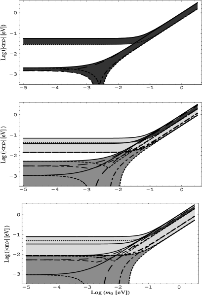
Figure 7: Effective Majorana neutrino mass $|\langle m\rangle|$ versus lightest mass $m_{0}$. The figure is taken from Ref. [79]. In the upper panel best fit values for the neutrino oscillation parameters have been used and only the phases $\beta_{1}$ and $\beta_{2}$ have been varied. (A non-zero best fit value for $s_{13}$ is used in this plot.) In the lower two panels the uncertainty in the determination of the oscillation parameters has been taken into account. For the details and for the precise meaning of the lines in the shaded regions, which correspond to CP-conserving choices of the phases $\beta_{1,2}$, see Ref. [79].

In order to plot $|\langle m\rangle|$ against $m_{0}$, the values of neutrino oscillation parameters are used as input. The phases $\beta_{1,2}$ are free parameters; for CP conservation the possible values of $\beta_{1,2}$ are zero or $\pi$. The plot of Fig. 7 has been taken from Ref. [79]. In the upper panel, best fit values of the neutrino oscillation parameters are used, whereas in the lower two panels the uncertainty in these parameters is taken into account. The lower band on the left sides of these panels correspond to the normal spectrum, whereas the upper band to the inverted spectrum.

What does this figure teach us? One can use experimental upper bounds on $|\langle m\rangle|$ and $m_{0}$ and compare with the allowed regions in the plot. It has been put forward in Ref. [81] that such a comparison, even if $(\beta\beta)_{0\nu}$ decay is not found experimentally, might reveal the neutrino nature: If the minimum of $|\langle m\rangle|$ predicted from $m_{\beta}$ and the oscillation parameters exceeds the experimental upper bound on $|\langle m\rangle|$, then the neutrino must have Dirac nature. There are, however, several difficulties with such a procedure: Other mechanisms for $(\beta\beta)_{0\nu}$ decay could destroy the validity of such a comparison; $m_{\beta}$ will not reach the non-degenerate neutrino mass region even with the KATRIN experiment, and the same difficulty applies to the region with $|\langle m\rangle|$ below 0.01 eV; moreover, imprecise determination of the oscillation parameters blur the picture as seen from the lower two panels of Fig. 7. However, the chances for this approach would be good, if the KATRIN experiment would find a non-zero $m_{\beta}$. On the other hand, assuming the validity of the Majorana hypothesis, Fig. 7 might give us information about the type of neutrino mass spectrum if $|\langle m\rangle|$ is measured or a sufficiently stringent experimental bound on it is derived [79].

Neutrino masses and cosmology:

A very interesting bound on the sum over all neutrino masses is provided by the large-scale structure of the universe [82] and the temperature fluctuations of the cosmic microwave background (CMB) [83]. Usually, energy densities $\rho_{i}$ in the universe are given as fractions $\Omega_{i}\equiv\rho_{i}/\rho_{\mathrm{cr}}$ of the critical energy density $\rho_{\mathrm{cr}}$ of the universe. Today’s energy density of non-relativistic neutrinos and antineutrinos is given by (see, for instance, [84])

$$\Omega_{\nu}h^{2}=\sum_{j}m_{j}/(93.5\>\mathrm{eV})\,,$$ (100)

where $h\simeq 0.7$ is the Hubble constant in units of 100 km s^-1 Mpc^-1. Of the three active neutrinos, at least two of them are non-relativistic today since $\sqrt{\Delta m^{2}_{\odot}}\sim 0.008$ eV and $\sqrt{\Delta m^{2}_{\mathrm{atm}}}\gg\sqrt{\Delta m^{2}_{\odot}}$, while the neutrino temperature today corresponds to $1.7\times 10^{-4}$ eV [84].

Roughly speaking, an upper bound on $\Omega_{\nu}$ is obtained in the following way. Hot dark matter tends to erase primordial density fluctuations. The theory of structure formation together with data on large-scale structures (distribution of galaxies and galaxy clusters), mainly from the 2 degree field Galaxy Redshift Survey [82], gives an upper bound on $\Omega_{\nu}/\Omega_{m}$, where $\Omega_{m}$ is the total matter density. On the other hand, data on the temperature fluctuations of the CMB can be evaluated with the so-called $\Lambda$CDM model (a flat universe with cold dark matter and a cosmological constant) and allows in this way to determine a host of quantities like $h$, $\Omega_{m}$, $\Omega_{b}$ (the baryon density), etc. Since the quantities extracted in this way agree rather well with determinations based on different methods and assumptions [83], the $\Lambda$CDM model is emerging as the standard model of cosmology [85]. Evaluation of the recent CMB results of the Wilkinson Microwave Anisotropy Probe (WMAP) and of the large-scale structure data give the impressive bound [83] $\Omega_{\nu}h^{2}<0.0076$ (95% CL); with Eq. (100) this bound is reformulated in terms of neutrino masses:

$$\sum_{j}m_{j}<0.7\;\mathrm{eV}\;(95\%\mathrm{CL}).$$ (101)

For a single neutrino we have thus $m_{j}<0.23$ eV, since neutrinos with masses in the range of a few tenths eV have to be degenerate.

Note that the $\Lambda$CDM model gives the result $\Omega_{m}\sim 0.3$ and $\Omega_{\Lambda}\sim 0.7$; the latter quantity is the energy density associated with the cosmological constant $\Lambda$. Furthermore, one finds $\Omega_{\nu}\>\mbox{\raisebox{-3.0pt}{$\stackrel{{\scriptstyle\displaystyle<}}{{\sim}}$}}\>0.015$ and $\Omega_{b}\sim 0.04\div 0.05$, thus the main contribution to $\Omega_{m}$ must consist of hitherto undetermined dark matter components.

3.5 Neutrino electromagnetic moments

The effective Hamiltonians for neutrinos with magnetic moments and electric dipole moments (electromagnetic moments) are given by the following expressions:

Dirac: $$\mathcal{H}_{\mathrm{em}}^{D}=\frac{1}{2}\bar{\nu}_{R}\lambda\,\sigma^{\mu\nu}\nu_{L}F_{\mu\nu}+\mathrm{H.c.},$$ (102)

Majorana: $$\mathcal{H}_{\mathrm{em}}^{M}=-\frac{1}{4}\nu_{L}^{T}C^{-1}\lambda\,\sigma^{\mu\nu}\nu_{L}F_{\mu\nu}+\mathrm{H.c.}$$ (103)

In the Majorana case, from $(C^{-1}\sigma^{\mu\nu})^{T}=C^{-1}\sigma^{\mu\nu}$ and the anticommutation property of $\nu_{L}$, it follows that $\lambda^{T}=-\lambda$ and only transition moments are allowed. In the Dirac case, the electromagnetic moment matrix $\lambda$ is an arbitrary $3\times 3$ matrix. Usually, a decomposition of $\lambda$ is made into $\lambda=\mu-id$ with $\mu^{\dagger}=\mu$ being the MM matrix and $d^{\dagger}=d$ the EDM matrix. However, since the neutrino mass eigenstates are experimentally not accessible, the distinction MM/EDM is completely unphysical in terrestrial experiments. This holds also largely for solar neutrinos, though in the evolution of the solar neutrino state the squares of the neutrino masses enter, and one can shift phases from the mixing matrix to the electromagnetic moment matrix and vice versa, which makes the distinction MM/EDM phase-convention-dependent. For a thorough discussion of this point see Ref. [86].

Bounds on $\lambda$ from solar and reactor neutrinos are obtained via elastic $\nu e^{-}$ scattering where, due to the helicity flip in the Hamiltonians (102) and (103), the cross section is the sum of the weak and electromagnetic cross sections [87]:

$$\frac{d\sigma}{dT}=\frac{d\sigma_{w}}{dT}+\frac{d\sigma_{\mathrm{em}}}{dT}\quad\mbox{with}\quad\frac{d\sigma_{\mathrm{em}}}{dT}=\frac{\alpha^{2}\pi}{m_{e}^{2}\mu_{B}^{2}}\left(\frac{1}{T}-\frac{1}{E}\right)\mu_{\mathrm{eff}}^{2}\,.$$ (104)

In the most general form, the effective MM is given by [86]

$$\mu_{\mathrm{eff}}^{2}=a_{-}^{\dagger}\lambda^{\dagger}\lambda a_{-}+a_{+}^{\dagger}\lambda\lambda^{\dagger}a_{+}\,.$$ (105)

In Eq. (104), $T$ is the kinetic energy of the recoil electron, $\mu_{B}$ is the Bohr magneton, and the flavour 3-vectors $a_{\pm}$ describe the neutrino helicity states at the detector. The expression (105) is basis-independent, thus it does not matter in which basis, flavour or mass basis, the quantities $\lambda$, $a_{\pm}$ and the Hamiltonians (102) and (103) are perceived [86].

In the following we will consider reactor and solar neutrinos. If the detector is close to the reactor, one simply has (in the flavour basis) $a_{-}=0$, $a_{+}=(1,0,0)^{T}$, as the reactor emits antineutrinos with positive helicity. For solar neutrinos, the effective MM will, in general, depend on the neutrino energy $E$. Bounds on the neutrino electromagnetic moments have been obtained from both reactor [88] and solar neutrinos [89, 90].

From now on, we concentrate on Majorana neutrinos, where the antisymmetric matrix $\lambda$ contains only three complex parameters (in the Dirac case there are nine parameters). Thus, $\lambda$ can be written as

$$\lambda_{\alpha\beta}=\varepsilon_{\alpha\beta\gamma}\Lambda_{\gamma}\,,$$ (106)

in either basis, flavour or mass basis. For the approximations used in the calculation of the effective MM for solar neutrinos and the LMA MSW solution, $\mu_{\mathrm{LMA}}^{2}$, we refer the reader to Ref. [91]. The result is given by

$$\mu_{\mathrm{LMA}}^{2}(E)=|\mathbf{\Lambda}|^{2}-|\Lambda_{2}|^{2}+P^{S}_{e1}\left(|\Lambda_{2}|^{2}-|\Lambda_{1}|^{2}\right).$$ (107)

The probability $P^{S}_{e1}$ is defined before Eq. (34). For reactor neutrinos the effective MM is immediately obtained as

$$\mu_{\mathrm{reactor}}^{2} = |\lambda_{e\mu}|^{2}+|\lambda_{e\tau}|^{2}=|\Lambda_{\mu}|^{2}+|\Lambda_{\tau}|^{2}$$ (108)

$$= |\mathbf{\Lambda}|^{2}-c_{12}^{2}|\Lambda_{1}|^{2}-s_{12}^{2}|\Lambda_{2}|^{2}-2s_{12}c_{12}|\Lambda_{1}||\Lambda_{2}|\cos\delta^{\prime}\,,$$

where the second line is derived from the first line by using $\mathbf{\Lambda}=U_{M}\tilde{\mathbf{\Lambda}}$. The phase $\delta^{\prime}$ is composed of $\delta^{\prime}=\arg(\Lambda_{1}^{*}\Lambda_{2})+\alpha_{2}-\alpha_{1}$ with the Majorana phases $\alpha_{j}$ defined in Eq. (90). Eq. (106) defines the vectors $\mathbf{\Lambda}=(\Lambda_{\alpha})$ and $\tilde{\mathbf{\Lambda}}=(\Lambda_{j})$ in the flavour and mass basis, respectively. The length of $\mathbf{\Lambda}$ occurs in both effective moments, Eqs. (107) and (108). Note, however, that

$$|\mathbf{\Lambda}|^{2}=\frac{1}{2}\mathrm{Tr}\,(\lambda^{\dagger}\lambda)\quad\Rightarrow\quad|\mathbf{\Lambda}|=|\tilde{\mathbf{\Lambda}}|\,,$$ (109)

i.e., the length of the vector of the electromagnetic moments is basis-independent.

In Ref. [91] a bound on $|\mathbf{\Lambda}|$ is derived, i.e., all three transition moments are bounded by using as input the rates of the solar neutrino experiments, the shape of Super-Kamiokande recoil electron energy spectrum and the results of reactor experiments at Bugey (MUNU) and Rovno [88]. As statistical procedure a Bayesian method is used with flat priors and minimization of $\chi^{2}$ with respect to $\theta_{12}$, $\Delta m^{2}_{\odot}$, $|\Lambda_{1}|$, $|\Lambda_{2}|$, $\delta^{\prime}$, in order to extract a probability distribution for $|\mathbf{\Lambda}|$. The details are given in Ref. [91], where the 90% CL bounds

$$|\mathbf{\Lambda}|<\bigg{\{}\begin{array}[]{cl}6.3\times 10^{-10}\mu_{B}&(\mbox{solar data})\,,\\ 2.0\times 10^{-10}\mu_{B}&(\mbox{solar}+\mbox{reactor data})\end{array}$$ (110)

are presented.

Some comments are at order [91]:

• We want to stress once more that the bounds in Eq. (110) apply to $|\mathbf{\Lambda}|^{2}=|\lambda_{e\mu}|^{2}+|\lambda_{\mu\tau}|^{2}+|\lambda_{\tau e}|^{2}=\sum_{j<k}|\lambda_{jk}|^{2}\,.$ Therefore, all transition moments are bounded in a basis-independent way.

• In Eq. (107), in the limit $P^{S}_{e1}\to 0$, the quantity $|\Lambda_{2}|$ drops out of the effective MM. Therefore, for small $P^{S}_{e1}$, solar neutrino data become less stringent for $|\Lambda_{2}|$ and thus for $|\mathbf{\Lambda}|$ as well. This is the case for Super-Kamiokande data (see the first bound in Eq. (110)) where $P^{S}_{e1}$ is small due to the relatively high neutrino energy (see Eq. (55)).

• Reactor data give a good bound on $|\Lambda_{2}|$ and are, therefore, complementary to present solar neutrino data.

• The BOREXINO experiment [92] could improve the second bound in Eq. (110) by nearly one order of magnitude because it is sensitive to relatively low neutrino energies where $P^{S}_{e1}\sim 0.5$.

4 Models for neutrino masses and mixing

4.1 Introduction and scope

For a start, we present the problems of model building for neutrino masses and mixing by asking appropriate questions and formulating answers, if available.

1. Can neutrino masses and mixing be accommodated in a model?
   This is no problem; the simplest possibility is given by the SM + 3 right-handed neutrino singlets $\nu_{R}$ + $L$ conservation which allows to accommodate arbitrary masses and mixing of Dirac neutrinos in complete analogy to the quark sector.

2. Why are neutrino masses much smaller than the charged lepton masses?
   There are two popular proposals for a solution to this problem:

   • Radiative neutrino masses;

   • Seesaw mechanism [93, 94].

3. Can one reproduce the special features of $\nu$ masses and mixing?
   Let us list the features one would like to explain:

   • $\theta_{\odot}\sim 34^{\circ}$ (large but non-maximal);

   • $\theta_{\mathrm{atm}}\simeq 45^{\circ}$;

   • $|U_{e3}|^{2}\equiv s_{13}^{2}\>\mbox{\raisebox{-3.0pt}{$\stackrel{{\scriptstyle\displaystyle<}}{{\sim}}$}}\>0.05$;

   • $\Delta m_{\odot}^{2}/\Delta m_{\mathrm{atm}}^{2}\sim 0.03$.

   We have used the obvious notation where the subscripts $\odot$ and atm refer to solar and atmospheric neutrinos, respectively.

To explain the listed features is the most difficult and largely unsolved task. There are myriads of textures or models—for reviews see Ref. [95]. One of the problems is that there are still not enough clues where to start model building.

Figure 8: Symbolical presentation of the variety of possibilities for model building. The upper two blocks show the two energy scales at which the symmetries, indicated in the three blocks below, could apply. RG eq stands for renormalization group equation, $\pm$ for with/without.

Symbolically, the difficulties of model building are presented in Fig. 8. If the symmetries apply at the GUT scale, the renormalization group equation transports relations from the GUT scale to the low scale; this transport could contribute to generate some of the desired features—for a review see Ref. [96]. It is completely unknown if the explanation of the features F1-4 is independent of general fermion mass problem or not. In the following we will assume independence.

The scope of the following sections is to discuss some simple extensions of the SM by addition of scalar multiplets and of right-handed neutrino singlets $\nu_{R}$. All these extensions will yield Majorana neutrino masses. We will only discuss the lepton sector.

4.2 The Standard Model with additional scalar multiplets

In the SM there are only two types of lepton multiplets:

$$\begin{array}[]{ccccl}&SU(2)&\!\!\times\!\!&\!U(1)&\\ D_{L}&\underline{\frac{1}{2}}&&Y=-1&\mbox{left-handed doublets}\\ \ell_{R}&\underline{0}&&Y=-2&\mbox{right-handed singlets}\end{array}$$

Here $Y$ is the hypercharge and the underlined numbers indicate the weak isospin of the multiplet.

By forming all possible leptonic bilinears one obtains the possible scalar gauge multiplets which can couple to fermions [97]:

$$\begin{array}[]{cr@{\,=\,}lccl}\bar{D}_{L}\otimes\ell_{R}&\underline{\frac{1}{2}}\otimes\underline{0}&\underline{\frac{1}{2}}&Y=-1&\>\phi&\mbox{doublet}\\ D_{L}\otimes D_{L}&\underline{\frac{1}{2}}\otimes\underline{\frac{1}{2}}&\underline{0}\oplus\underline{1}&Y=-2&\left\{\begin{array}[]{c}\eta^{+}\\ \!\!\Delta\end{array}\right.&\!\!\!\begin{array}[]{l}\mbox{singlet}\\ \mbox{triplet}\end{array}\\ \ell_{R}\otimes\ell_{R}&\underline{0}\otimes\underline{0}&\underline{0}&Y=-4&\quad k^{++}&\mbox{singlet}\end{array}$$

The hypercharge in this table refers to the leptonic bilinear. In the following we will discuss extensions of the SM with these scalar multiplets (except the trivial extension where only Higgs doublets are added).

The Zee model:

This model [98, 99] is defined as SM with $2\phi$ + $\eta^{+}$ and, therefore, has the Lagrangian

$$\mathcal{L}=\cdots+\left[f_{\alpha\beta}D_{\alpha L}^{T}C^{-1}i\tau_{2}D_{\beta L}\,\eta^{+}-\mu\,\phi_{1}^{\dagger}\tilde{\phi}_{2}\eta^{+}+\mbox{H.c.}\right],$$ (111)

where the dots indicate the SM part and terms of the Higgs potential which are not interesting for the following discussion. Note the antisymmetry of the coupling matrix: $f_{\alpha\beta}=-f_{\beta\alpha}$.

Since no fermionic multiplets have been added to the SM, the ensuing neutrino masses can only be of Majorana type. Thus the total lepton number $L$ must be broken, otherwise neutrino masses will be strictly forbidden. Let us assign a lepton number to $\eta^{+}$ from its Yukawa couplings in Eq. (111). Then we have the following list of lepton numbers of the multiplets of the Zee model:

$$\begin{array}[]{c|cccc}&D_{L}&\ell_{R}&\phi_{1,2}&\eta^{+}\\ \hline\cr L&1&1&0&-2\end{array}$$ (112)

Thus, $L$ is indeed explicitly violated by the term $\phi_{1}^{\dagger}\tilde{\phi}_{2}\eta^{+}$ in the Lagrangian. Such a term can only be formed if two Higgs doublets are present (if $\phi_{1}=\phi_{2}=\phi$, then $\phi^{\dagger}\tilde{\phi}\equiv 0$). In the Zee model a neutrino mass matrix $\mathcal{M}_{\nu}$ appears at the 1-loop level.

A lot of work has been done on the restricted Zee model [100] where only one Higgs doublet, say $\phi_{1}$, couples to the leptons. In this particularly simple version one has $\mathcal{M}_{\nu}\propto\left((m_{\alpha}^{2}-m_{\beta}^{2})f_{\alpha\beta}\right)$, where $m_{\alpha,\beta}$ denote the charged lepton masses. Note that without loss of generality we have chosen a basis where the charged lepton mass matrix is diagonal. The restricted Zee model is practically ruled out now because it allows only maximal solar mixing [101]; furthermore, it requires serious fine-tuning, namely $m_{\tau}^{2}|f_{e\tau}|\simeq m_{\mu}^{2}|f_{e\mu}|$; finally, the smallness of the neutrino masses has to be achieved by $|f_{\alpha\beta}|\>\mbox{\raisebox{-3.0pt}{$\stackrel{{\scriptstyle\displaystyle<}}{{\sim}}$}}\>10^{-4}$. If both $\phi_{1,2}$ couple to the leptons, then non-maximal solar mixing is admitted [102], the fine-tuning problem is somewhat alleviated, but the third point remains. For further recent literature on the Zee model see, e.g. Ref. [103]

The Zee-Babu model:

This model is defined as [99, 104] SM + $\eta^{+}$ + $k^{++}$ and has the Lagrangian

$$\begin{array}[]{rcl}\mathcal{L}&=&\cdots+\left[f_{\alpha\beta}D_{\alpha L}^{T}C^{-1}i\tau_{2}D_{\beta L}\,\eta^{+}\right.\\[1.42262pt] &&\left.+h_{\alpha\beta}\ell_{\alpha R}^{T}C^{-1}\ell_{\beta R}\,k^{++}-\mu\,\eta^{-}\eta^{-}k^{++}+\mbox{H.c.}\right]\end{array}$$ (113)

with a symmetric coupling matrix $h_{\alpha\beta}=h_{\beta\alpha}$. In addition to the assignments (112), we have $L(k^{++})=-2$. Again, $L$ must be explicitly broken, which is now achieved by the $\mu$-term in Eq. (113).

Since in this model there is only one Higgs doublet, $L$ is still conserved at the 1-loop level (see previous section on the Zee model) and the neutrino mass matrix appears at the 2-loop level: $\mathcal{M}_{\nu}\propto\tilde{f}\hat{m}_{\ell}{\tilde{h}}^{*}\hat{m}_{\ell}\tilde{f}$ with $\tilde{f}=(f_{\alpha\beta})$, $\tilde{h}=(h_{\alpha\beta})$ and $\hat{m}_{\ell}=\mbox{diag}\,(m_{e},m_{\mu},m_{\tau})$. This model has the following properties [105]. Since $\tilde{f}$ is antisymmetric, the lightest neutrino mass is zero; the solar LMA MSW solution and, e.g., a hierarchical neutrino mass spectrum require the fine-tuning $|h_{\mu\mu}|:|h_{\mu\tau}|:|h_{\tau\tau}|\simeq 1:(m_{\mu}/m_{\tau}):(m_{\mu}/m_{\tau})^{2}$; all scalar masses are in the TeV range; in order to reproduce the neutrino masses inferred from atmospheric and solar data one needs $|f_{\alpha\beta}|$, $|h_{\alpha\beta}|\>\mbox{\raisebox{-3.0pt}{$\stackrel{{\scriptstyle\displaystyle<}}{{\sim}}$}}\>0.1$, thus neutrino masses are naturally small as a consequence of the 2-loop mechanism; finally, rare decays like $\tau\to 3\mu$, $\mu\to e\gamma$ should be within reach of forthcoming experiments.

We note that from the Zee model and Zee-Babu model we have seen that models with radiative neutrino mass generation are prone to excessive fine-tuning because the hierarchy of the charged lepton masses works against the features needed in the neutrino sector.

The triplet model:

This model is defined by adding a scalar triplet $\Delta$ to the SM and has the Lagrangian

$$\begin{array}[]{rcl}\mathcal{L}&=&\cdots+\left[\frac{1}{2}g_{\alpha\beta}D_{\alpha L}^{T}C^{-1}i\tau_{2}\Delta D_{\beta L}+\mbox{H.c.}\right]\\ &&-\frac{1}{2}M^{2}\mbox{Tr}\,\Delta^{\dagger}\Delta-\left(\mu\,\phi^{\dagger}\Delta\tilde{\phi}+\mbox{H.c.}\right)\end{array}$$ (114)

The electric charge eigenfields and the VEV of the triplet are given as

$$\Delta=\left(\begin{array}[]{cc}H^{+}&\sqrt{2}H^{++}\\ \sqrt{2}H^{0}&-H^{+}\end{array}\right),\quad\langle H^{0}\rangle_{0}=\frac{1}{\sqrt{2}}v_{T}\,,$$ (115)

respectively. Note that $g_{\alpha\beta}=g_{\beta\alpha}$. As in the previous two models, we can make the assignment $L(\Delta)=-2$, then $L$ is explicitly broken by the $\mu$-term in Eq. (114). The original model without the $\mu$-term and spontaneous $L$ breaking [106] is ruled out by the non-discovery of the Goldstone boson and a light scalar at LEP. This model leads to the tree-level neutrino mass matrix $\mathcal{M}_{\nu}=v_{T}(g_{\alpha\beta})$. The LEP data require $|v_{T}/v|\>\mbox{\raisebox{-3.0pt}{$\stackrel{{\scriptstyle\displaystyle<}}{{\sim}}$}}\>0.03$ [107], where $v$ is the VEV of the SM Higgs doublet. However, if the coupling constants $g_{\alpha\beta}$ are about $0.01\div 0.1$, then in order to obtain small neutrino masses the triplet VEV must be much smaller, namely $v_{T}\sim 0.1\div 1$ eV. There are two ways to get a small $v_{T}$: Firstly, one can assume that $M,\>|\mu|\gg v$, then $|v_{T}|\simeq|\mu|v^{2}/M^{2}$ (scalar or type II seesaw mechanism) [94, 109]; secondly, with $M\sim v,\>|\mu|\ll v$ one has $|v_{T}|\sim|\mu|$ [108]. In some sense the mechanism for obtaining small neutrino masses in the triplet model is analogous to the seesaw mechanism [93, 94] (see subsequent subsection) since in both cases one has to introduce a second scale much larger (smaller) than the electroweak scale in order to generate small neutrino masses.

4.3 The seesaw mechanism

The seesaw mechanism [93, 94] is implemented in the simplest way in the SM + $3\,\nu_{R}$ + $L$ violation. This is primarily an extension in the fermion sector of the SM. Note that one could also choose two or more than three right-handed singlets $\nu_{R}$. The starting point is the Lagrangian

$$\begin{array}[]{rcl}\mathcal{L}&=&\cdots-\left[\sum_{j}\left(\bar{\ell}_{R}\phi_{j}^{\dagger}\Gamma_{j}+\bar{\nu}_{R}{\tilde{\phi}}_{j}^{\dagger}\Delta_{j}\right)D_{L}+\mbox{H.c.}\right]\\[5.69054pt] &&+\left(\frac{1}{2}\,\nu_{R}^{T}C^{-1}\!M_{R}^{*}\nu_{R}+\mbox{H.c.}\right),\end{array}$$ (116)

where the mass matrix $M_{R}$ of the right-handed singlets must be symmetric due to their fermionic anticommutation property. The number $n_{H}$ of Higgs doublets is irrelevant for the seesaw mechanism. Defining the mass matrices

$$M_{\ell}=\frac{1}{\sqrt{2}}\sum_{j}v_{j}^{\ast}\Gamma_{j}\,,\quad M_{D}=\frac{1}{\sqrt{2}}\sum_{j}v_{j}\Delta_{j}\,,$$ (117)

where $M_{\ell}$ is the mass of the charged leptons and $M_{D}$ is the so-called “Dirac mass matrix” for the neutrinos, the total Majorana mass matrix for all six left-handed fields $\omega_{L}$ is given by [110]

$$\mathcal{M}_{D+M}=\left(\begin{array}[]{cc}0&M_{D}^{T}\\ M_{D}&M_{R}\end{array}\right)\quad\mbox{with}\quad\omega_{L}=\left(\begin{array}[]{c}\nu_{L}\\ C(\bar{\nu}_{R})^{T}\end{array}\right).$$ (118)

The VEVs $v_{j}$ fulfill $v=\sqrt{|v_{1}|^{2}+\ldots|v_{n_{H}}|^{2}}=(\sqrt{2}\,G_{F})^{-1/2}\simeq 246$ GeV.

The basic assumption for implementing the seesaw mechanism is $m_{D}\ll m_{R}$, where $m_{D,R}$ are the scales of $M_{D,R}$, respectively. With this assumption, one obtains the mass matrix of the light neutrinos

$$\mathcal{M}_{\nu}=-M_{D}^{T}M_{R}^{-1}M_{D}\,,$$ (119)

which is valid up to corrections of order $(m_{D}/m_{R})^{2}$. The mass matrix of heavy neutrinos is given by $\mathcal{M}_{\nu}^{\mathrm{heavy}}=M_{R}$. Diagonalizing the mass matrices by

$$(U_{R}^{\ell})^{\dagger}M_{\ell}U_{L}^{\ell}=\hat{m}_{\ell}\,,\quad V^{T}\mathcal{M}_{\nu}V=\hat{m}\,,$$ (120)

the neutrino mixing matrix for the light neutrinos is given by

$$U_{M}=(U_{L}^{\ell})^{\dagger}V\,.$$ (121)

As discussed earlier, phases multiplying $U_{M}$ from the left are unphysical because they can be absorbed into the charged lepton fields.

The seesaw mechanism contains three sources for neutrino mixing: $M_{\ell}$, $M_{D}$ and $M_{R}$. Therefore, it is a rich playground for model building. It can also be combined with radiative neutrino mass generation—for an example see next subsection. Let us discuss the order of magnitude of the scale $m_{R}$. If we choose as a typical neutrino mass $m_{\nu}\sim\sqrt{\Delta m^{2}_{\mathrm{atm}}}\sim 0.05$ eV and assume $m_{D}\sim m_{\mu,\tau}$, we obtain $m_{R}\sim 10^{8}\div 10^{11}$ GeV. On the other hand, if $m_{D}$ is of the order of the electroweak scale, then $m_{R}\sim 10^{15}$ GeV and there could be a possibility to identify it with the GUT scale.

4.4 Combining the seesaw mechanism with radiative mass generation

Let us now consider the SM with two Higgs doublets $\phi_{1,2}$, add a single field $\nu_{R}$ and allow for $L$ violation [111, 112]. We do not employ any flavour symmetry.

In this case the Yukawa coupling matrices $\Delta_{1,2}$ and $M_{D}$ are $1\times 3$ matrices (vectors!). Here we give a precise meaning to the scale $m_{D}$ and identify it with the length of the vector $M_{D}$. $L$ violation is induced by the Majorana mass term with mass $M_{R}\gg m_{D}$ of the neutrino singlet $\nu_{R}$. Then at the tree level the seesaw mechanism is operative:

$$\mbox{Tree level:}\quad m_{1}=m_{2}=0\,,\;m_{3}\simeq m_{D}^{2}/M_{R}\,.$$ (122)

That two masses are zero at the tree level is a consequence of $M_{D}$ being a $1\times 3$ matrix, which, therefore, maps two vectors onto 0; this feature is then operative in $\mathcal{M}_{D+M}$ (118) and $\mathcal{M}_{\nu}$ (119).

At 1-loop level, $m_{2}$ becomes non-zero by neutral-scalar exchange, bit $m_{1}$ remains zero:

$$\mbox{1-loop:}\quad m_{1}=0\,,\,\;m_{2}\sim\frac{1}{16\pi^{2}}\,m_{3}\,\frac{M_{0}^{2}}{v^{2}}\ln\,(M_{R}/M_{0})^{2}\,.$$ (123)

In this order-of-magnitude relation for $m_{2}$ [112], the mass $M_{0}\sim v$ is a typical scalar mass (there are three physical neutral scalars in this model). A general discussion for arbitrary numbers of left-handed lepton doublets, right-handed neutrinos singlets and Higgs doublets is found in [111]. The full calculation of the dominant 1-loop corrections to the seesaw mechanism is presented in [113].

The model has the following properties. It predicts a hierarchical spectrum, therefore $\sqrt{\Delta m^{2}_{\odot}/\Delta m^{2}_{\mathrm{atm}}}\simeq m_{2}/m_{3}\stackrel{{\scriptstyle\mathrm{exp.}}}{{\sim}}0.17$. It gives the correct order of magnitude of $m_{2}/m_{3}$ with $1/16\pi^{2}\simeq 0.0063$, $M_{0}^{2}/v^{2}\sim 1$, $\ln(M_{R}/M_{0})\sim 10$. The most interesting property of these 1-loop corrections to the seesaw mechanism is the fact that the suppression relative to the tree level terms is given solely by the loop integral factor $1/16\pi^{2}$ [111, 113]. The mixing angles are undetermined, but without fine-tuning they will be large in general. Consequently, the model has no argument for $\theta_{\mathrm{atm}}\simeq 45^{\circ}$ and small angle $\theta_{13}$; these must be reproduced by tuning the parameters of the model. This is easily achieved because in good approximation $|U_{\alpha 3}|=|M_{D\alpha}|/m_{D}$ [112].

It is interesting to note that R-parity-violating supersymmetric models have a built-in seesaw mechanism where the heavy Majorana neutrinos are replaced by the neutralinos which are also Majorana particles. See, e.g., Ref. [114] and citations therein.

4.5 A model for maximal atmospheric neutrino mixing

Her we want to discuss a model based on tree-level seesaw masses. While in the previous model the emphasis was on explaining the ratio $\Delta m^{2}_{\odot}/\Delta m^{2}_{\mathrm{atm}}$ and we assumed to obtain the mixing angles by tuning of model parameters, here we take the opposite attitude. One of the problems of obtaining maximal atmospheric neutrino mixing and large but non-maximal solar neutrino mixing by a symmetry is that the mixing matrix (121) has a contribution also from the charged lepton sector. Now we introduce a framework where this problem is avoided by having $M_{R}$ as the only source of neutrino mixing.

The framework:

We start with the Lagrangian (116) and allow for an arbitrary number $n_{H}$ of Higgs doublets. Then how can one avoid flavour-changing interactions via tree-level scalar interactions? We assume that the family lepton numbers $L_{e,\mu,\tau}$ are conserved in all terms of dimension 4 in the Lagrangian but $L_{\alpha}$ is softly broken by the $\nu_{R}$ mass term. This allows one to kill several birds with one stone: Flavour-changing neutral interactions are forbidden at the tree level, $M_{\ell}$ and $M_{D}$ are diagonal and neutrino mixing stems exclusively from $M_{R}$ [115], as announced above. However, soft breaking of lepton numbers occurs at the high scale $m_{R}$. It has been shown in Ref. [116] that this assumption yields a perfectly viable theory with interesting properties: All 1-loop flavour-changing vertices are finite because of soft $L_{\alpha}$ breaking; for $n_{H}>1$, such vertices where the boson leg is a neutral scalar and the exchanged boson is a charged scalar do not decouple in the limit $m_{R}\to\infty$ (for $n_{H}=1$ there is decoupling); diagrams with a $\gamma$ or a $Z$ and box diagrams always decouple. As a consequence, the amplitudes of $\mu\to e\gamma$, $Z\to e^{-}\mu^{+},\ldots$ are suppressed by $1/m_{R}^{2}$, whereas, e.g., the amplitude of $\mu\to 3e$ tends to a constant for $m_{R}\to\infty$ and is suppressed—though much less than the previous amplitudes—because it contains a product of four Yukawa couplings. The decay rate of the latter process in this framework might be within reach of forthcoming experiments. For details see Ref. [116].

Maximal atmospheric neutrino mixing:

Within the framework of soft $L_{\alpha}$-breaking we introduce now a $\mathbbm{Z}_{2}$ symmetry:

$$\mathbbm{Z}_{2}:\quad D_{\mu L}\leftrightarrow D_{\tau L},\>\nu_{\mu R}\leftrightarrow\nu_{\tau R},\>\mu_{R}\leftrightarrow\tau_{R}\,.$$ (124)

This symmetry makes $M_{D}$ and $M_{R}$ $\mathbbm{Z}_{2}$-invariant and, therefore, transfers to the neutrino mass matrix $\mathcal{M}_{\nu}$. Thus we obtain the result

$$\mathcal{M}_{\nu}=\left(\begin{array}[]{ccc}x&y&y\\ y&z&w\\ y&w&z\end{array}\right)\;\Rightarrow\;U=\left(\begin{array}[]{ccc}\scriptstyle\cos\theta&\scriptstyle\sin\theta&\scriptstyle 0\\ -\frac{\sin\theta}{\sqrt{2}}&\frac{\cos\theta}{\sqrt{2}}&\frac{1}{\sqrt{2}}\\ \frac{\sin\theta}{\sqrt{2}}&-\frac{\cos\theta}{\sqrt{2}}&\frac{1}{\sqrt{2}}\end{array}\right),$$ (125)

where $\theta\equiv\theta_{12}$ is the solar mixing angle. Summarizing, we have constructed a model where the solar mixing angle is free and without fine-tuning it will be large but non-maximal; atmospheric mixing is maximal; $|U_{e3}|=s_{13}=0$.

The above results are stable under radiative corrections because the mass matrix (125) was realized by the symmetries $U(1)_{L_{e}}\times U(1)_{L_{\mu}}\times U(1)_{L_{\tau}}$, which are softly broken, and $\mathbbm{Z}_{2}$, which has to be broken spontaneously in order to achieve $m_{\mu}\neq m_{\tau}$. This can be done with a minimum of three Higgs doublets and an auxiliary $\mathbbm{Z}^{\prime}_{2}$, without destroying the form of the mass matrix (125) [115]. Since the $\mathbbm{Z}_{2}$ of Eq. (124) does not commute with $L_{\mu,\tau}$, the full group generated by our symmetries is non-abelian [117]. The essential features of this model can be embedded in an $SU(5)$ GUT [117].

5 Conclusions

In recent years we have witnessed great progress in neutrino physics. Eventually, it has been confirmed that the solar neutrino puzzle is solved by neutrino oscillations, first conceived by Bruno Pontecorvo in 1957. At the same time, matter effects in neutrino oscillations—as occurring in the LMA MSW solution—have turned out to play a decisive role. It is firmly believed that also the atmospheric neutrino deficit problem is solved by neutrino oscillations though for the time being the final proof is still missing but is expected to be provided soon by LBL experiments.

Despite the great progress, which provides us with a first glimpse beyond the SM, there are still many things we would like to know. For instance, Are neutrinos Dirac or Majorana particles? What are the absolute neutrino masses? Of what type is the neutrino mass spectrum? Do neutrinos have sizeable magnetic moments?

As for field-theoretical models of neutrino masses and mixing, theorists are groping in the dark. As it has turned out, neutrino mass spectra and the neutrino mixing matrix are very different from the quark sector. Though there are many ideas, very few of them account naturally for some of the neutrino properties. Despite the big increase in our knowledge about neutrinos even basic questions for model building have no answer at the moment. Some of the basic questions are the following: Is the neutrino mass and mixing problem independent of the general fermion mass problem? Are neutrino masses small by radiative, seesaw or other mechanisms? Is the solution for the neutrino mass and mixing problem situated at the TeV scale or the GUT scale? Do we need a flavour symmetry for its solution and, if yes, of what type is this symmetry?

We want to stress that it is no problem to accommodate neutrino masses and mixing in theories, but the problem is to explain the specific features for neutrinos. As for the neutrino nature, there is a theoretical bias toward Majorana nature, e.g. from the seesaw mechanism and GUTs, in particular, from GUTs based on $SO(10)$. For the time being, there are simply not enough clues for a definite mechanism for neutrino masses and mixing. Among others, possible future clues provided by experiment would be an atmospheric mixing angle very close to $45^{\circ}$, which would point toward a non-abelian flavour symmetry; knowledge of the value of $|U_{e3}|=s_{13}$ and the neutrino mass spectrum, which would teach us more about the mass matrix; discovery of scalars with masses  $\stackrel{{\scriptstyle\displaystyle<}}{{\sim}}$  1 TeV, which would show that fermion masses are most probably generated by the Higgs mechanism; discovery of SUSY partners of ordinary particles, which would assure us that we have to take SUSY into account in model building. Evidence for flavour-changing decays like $\mu\to e\gamma$, $\mu\to 3e$, etc. would also give a valuable input.

At any rate, ongoing and future experiments will continue to provide us with exciting results, which will enhance the prospects of constructing viable mechanisms for explaining the specific neutrino features.

Acknowledgements: I wish to thank the Organizing Committee for the invitation to Schladming and A. Bartl, G. Ecker, M. Hirsch and H. Neufeld for discussions.

References

- [1] A.Yu. Smirnov, Talk given at the International Workshop NOON2003, February 10–14, 2003, Kanazawa, Japan, hep-ph/0306075; Talk given at the 11th Workshop on Neutrino Telescopes, Venice, March 11–14, 2003, hep-ph/0305106.
- [2] S. Goswami, Pramana 60, 261 (2003) [hep-ph/0305111].
- [3] C. Giunti, hep-ph/0305139.
- [4] G. Drexlin, Contribution to these proceedings.
- [5] J.N. Bahcall, S. Basu and M.P. Pinsonneault, Phys. Lett. B 433, 1 (1998); Astrophys. J. 555, 990 (2001).
- [6] SNO Collaboration, Q.R. Ahmad et al., Phys. Rev. Lett. 89, 011301 (2002) [nucl-ex/0204008].
- [7] KamLAND Collaboration, K. Eguchi et al., Phys. Rev. Lett. 90, 021802 (2003) [hep-ex/0212021].
- [8] S.M. Bilenky and B. Pontecorvo, Phys. Rep. 41, 225 (1978).
- [9] S.M. Bilenky, hep-ph/9908335.
- [10] L.B. Okun, M.G. Schepkin and I.S. Tsukerman, Nucl. Phys. B 650, 443 (2003); Err. ibid. 656, 255 (2003) [hep-ph/0211241].
- [11] S.M. Bilenky and S.T. Petcov, Rev. Mod. Phys. 59, 671 (1987).
- [12] S.M. Bilenky, C. Giunti and W. Grimus, Prog. Part. Nucl. Phys. 43, 1 (1999) [hep-ph/9812360].
-
[13]
P.B. Pal, Int. J. Mod. Phys. A 7, 5387 (1992);
K. Zuber, Phys. Rept. 305, 295 (1998);
P. Fisher, B. Kayser, and K. S. McFarland, Ann. Rev. Nucl. Part. Sci. 49, edited by C. Quigg, V. Luth, and P. Paul (Annual Reviews, Palo Alto, California, 1999), p. 481;
M. Gonzalez-Garcia and Y. Nir, Rev. Mod. Phys. 75, 345 (2003) [hep-ph/0202058]. -
[14]
R.N. Mohapatra and P.B. Pal,
Massive Neutrinos in Physics and Astrophysics,
World Scientific Lecture Notes in Physics, Vol. 41
(World Scientific, 1991);
C.W. Kim and A. Pevsner, Neutrinos in Physics and Astrophysics, Contemporary Concepts in in Physics, Vol. 8 (Academic Press, 1993). - [15] L. Wolfenstein, Phys. Rev. D 17, 2369 (1978); ibid. 20, 2634 (1979).
- [16] S.P. Mikheyev and A.Yu. Smirnov, Yad. Fiz. 42, 1441 (1985) [Sov. J. Nucl. Phys. 42, 913 (1985)]; Il Nuovo Cim. C 9, 17 (1986).
- [17] LSND Collaboration, A. Aguilar et al., Phys. Rev. D 64, 112007 (2001) [hep-ex/0104049].
- [18] M. Maltoni, T. Schwetz, M.A. Tórtola and J.W.F. Valle, Nucl. Phys. B 643, 321 (2002) [hep-ph/0207157]; in Proc. of 30th International Meeting on Fundamental Physics (IMFP2002), Jaca, Spain, January 28–February 1, 2002, Nucl. Phys. B (Proc. Suppl.) 114, 203 (2003) [hep-ph/0209368].
- [19] M. Sorel, J. Conrad and M. Shaevitz, hep-ph/0305255.
- [20] CHOOZ Experiment, M. Apollonio et al., Eur. Phys. J. C 27, 331 (2003) [hep-ex/0301017].
- [21] Palo Verde Experiment, F. Boehm et al., Phys. Rev. D 64, 112001 (2001) [hep-ex/0107009].
- [22] M. Zrałek, Acta Phys. Pol. B 29, 3925 (1998) [hep-ph/9810543].
- [23] M. Beuthe, Phys. Rept. 375, 105 (2003) [hep-ph/0109119].
- [24] J. Rich, Phys. Rev. D 48, 4318 (1993).
- [25] M. Beuthe, Phys. Rev. D 66, 013003 (2002) [hep-ph/0202068].
- [26] C. Giunti, C.W. Kim and J.A. Lee, Phys. Rev. D 48, 4310 (1993) [hep-ph/9305276].
- [27] W. Grimus and P. Stockinger, Phys. Rev. D 54, 3414 (1996) [hep-ph/9603430].
- [28] H. Lipkin, Phys. Lett. B 348, 304 (1995) [hep-ph/9501269].
- [29] W. Grimus, P. Stockinger and S. Mohanty, Phys. Rev. D 59, 013011 (1999) [hep-ph/9807442].
- [30] H. Lipkin, hep-ph/0304187.
- [31] L. Stodolsky, Phys. Rev. D 58, 036006 (1998) [hep-ph/9802387].
- [32] B. Kayser, Phys. Rev. D 24, 110 (1981).
- [33] W. Grimus, S. Mohanty P. and Stockinger, Phys. Rev. D 61, 033001 (2000) [hep-ph/9904285].
- [34] K. Kiers, S. Nussinov and N. Weiss, Phys. Rev. 53, 537 (1996) [hep-ph/9506271].
- [35] C. Giunti, hep-ph/0302026.
- [36] S.P. Mikheyev and A.Yu. Smirnov, Prog. Part. Nucl. Phys. 23, 41 (1989).
- [37] H.A. Bethe, Phys. Rev. Lett. 56, 1305 (1986).
- [38] J.J. Sakurai, Advanced Quantum Mechanics (Addison-Wesley, Reading, Massachusetts, 1967), p. 62.
- [39] J. Liu, Phys. Rev. D 45, 1428 (1992).
-
[40]
W. Grimus and T. Scharnagl, Mod. Phys. Lett. A 8, 1943 (1993);
B. Bekman, J. Gluza, J. Holeczek, J. Syska and M. Zrałek, Phys. Rev. D 66, 093004 (2002) [hep-ph/0207015]. - [41] M.C. Gonzalez-Garcia and C. Peña-Garay, in Proc. of XIXth International Conference on Neutrino Physics and Astrophysics, Sudbury, Canada, 16-21 June 2000, Nucl. Phys. B (Proc. Suppl.) 91, 80 (2001) [hep-ph/0009041].
- [42] S. Choubey, A. Bandyopadhyay, S. Goswami and D.P. Roy, Talk given at Conference on Physics beyond the Standard Model: Beyond the Desert 02, Oulu, Finland, 2–7 June 2002, hep-ph/0209222.
- [43] L.I. Schiff, Quantum Mechanics (McGraw-Hill, 1987).
- [44] W.C. Haxton, Phys. Rev. Lett. 57, 1271 (1986).
- [45] S.J. Parke, Phys. Rev. Lett. 57, 1275 (1986).
- [46] T.K. Kuo and J. Pantaleone, Rev. Mod. Phys. 61, 937 (1989).
- [47] S.P. Mikheyev and A.Yu. Smirnov, Sov. Phys. JETP 65, 230 (1987).
- [48] A. Friedland, Phys. Rev. D 64, 013008 (2001) [hep-ph/0010231].
- [49] J.N. Bahcall, M.C. Gonzalez-Garcia and C. Peña-Garay, JHEP 0207, 054 (2002) [hep-ph/0204314].
- [50] Cheng-Wei Chiang and L. Wolfenstein, Phys. Rev. D 63 057303 (2001) [hep-ph/0010213].
- [51] S.M. Bilenky, C. Giunti, J.A. Grifols and E. Masso, Phys. Rept. 379, 69 (2003) [hep-ph/0211462].
- [52] Particle Data Group, K. Hagiwara et al., Phys. Rev. D 66, 010001 (2002).
-
[53]
G.L. Fogli et al., Phys. Rev. D 66, 093008 (2002)
[hep-ph/0208026];
M.C. Gonzalez-Garcia and C. Peña-Garay, hep-ph/0306001. - [54] M. Shiozawa, Talk given at the XXth International Neutrino Conference on Neutrino Physics and Astrophysics, Munich, May 25–30, 2002, Transparencies at http://neutrino2002.ph.tum.de.
- [55] T. Nakaya, in Proc. of XXth International Neutrino Conference on Neutrino Physics and Astrophysics, Munich, May 25–30, 2002, Nucl. Phys. B (Proc. Suppl.) 118, 210 (2003).
- [56] S. Geer, Phys. Rev. D 57, 6989 (1998); Err. ibid. 59, 039903 (1999) [hep-ph/9712290].
- [57] V. Barger, S. Geer, R. Raja and K. Whisnant, Phys. Rev. D 62, 013004 (2000) [hep-ph/9911524].
- [58] M. Freund, M. Lindner, S.T. Petcov and A. Romanino, Nucl. Phys. B 578, 27 (2000) [hep-ph/9912457].
- [59] P. Huber, M. Lindner and W. Winter, Nucl. Phys. B 645, 3 (2002) [hep-ph/0204352].
- [60] M. Lindner, in Proc. of XXth International Neutrino Conference on Neutrino Physics and Astrophysics, Munich, May 25–30, 2002, Nucl. Phys. B (Proc. Suppl.) 118, 199 (2003) [hep-ph/0210377].
-
[61]
I. Schur, Am. J. Math. 67, 472 (1945);
see also B. Zumino, J. Math. Phys. 3, 1055 (1962);
W. Grimus and G. Ecker, J. Phys. A: Math. Gen. 21, 2825 (1988). -
[62]
L. Wolfenstein, Phys. Lett. 107B, 77 (1981);
S.M. Bilenky, N.P. Nedelcheva and S.T. Petcov, Nucl. Phys. B 247, 61 (1984);
B. Kayser, Phys. Rev. D 30, 1023 (1984). - [63] M. Fukugita and T. Yanagida, Phys. Lett. B 174, 45 (1986).
-
[64]
A. Pilaftsis, Int. J. Mod. Phys. A 14, 1811 (1999)
[hep-ph/9812256];
W. Buchmüller and M. Plümacher, Int. J. Mod. Phys. A 15, 5047 (2000) [hep-ph/0007176];
W. Buchmüller, Lectures given at the 2001 European School of High-Energy Physics, Beatenberg, Switzerland, hep-ph/0204288. - [65] J.A. Casas and A. Ibarra, Nucl. Phys. B 618, 171 (2002) [hep-ph/0103065].
-
[66]
G.C. Branco, T. Morozumi, B.M. Nobre and M.N. Rebelo,
Nucl. Phys. B 617, 475 (2001) [hep-ph/0107164];
M.N. Rebelo, Phys. Rev. D 67, 013008 (2003) [hep-ph/0207236] - [67] S. Pascoli, S.T. Petcov and W. Rodejohann, hep-ph/0302054.
- [68] V.I. Tretyak and Y.G. Zdesenko, Atomic Data and Nuclear Data Tables 80, 83 (2002).
- [69] Heidelberg-Moscow Collaboration, H.V. Klapdor-Kleingrothaus et al., Eur. Phys. J. A 12, 147 (2001).
- [70] S.R. Elliot and P. Vogel, Ann. Rev. Nucl. Sci. 52, 115 (2002) [hep-ph/0202264].
- [71] R.N. Mohapatra, in Proc. of XVIIIth International Neutrino Conference on Neutrino Physics and Astrophysics, Takayama, Japan, June 4–9, 1998, Nucl. Phys. B (Proc. Suppl.) 77, 376 (1999) [hep-ph/9808284].
- [72] IGEX Collaboration, C.E. Aalseth et al., Phys. Rev. D 65, 092007 (2002) [hep-ex/0202026].
-
[73]
R.N. Mohapatra, Phys. Rev. D 34, 3457 (1986);
M. Hirsch, H.V. Klapdor-Kleingrothaus and S.G. Kovalenko, Phys. Rev. Lett. 75, 17 (1995). - [74] M.B. Smy (Super-Kamiokande Collaboration), in Proc. of XXth International Neutrino Conference on Neutrino Physics and Astrophysics, Munich, May 25–30, 2002, Nucl. Phys. B (Proc. Suppl.) 118, 199 (2003) [hep-ex/0208004].
- [75] J. Schechter and J.W.M. Valle, Phys. Rev. D 25, 2951 (1982).
- [76] E. Takasugi, Phys. Lett. 149B, 372 (1984).
- [77] H. Päs and T.J. Weiler, Phys. Rev. D 63, 113015 (2001) [hep-ph/0101091]; Talk presented at SUSY02, 10th International Conference on Supersymmetry and Unification of Fundamental Interactions, DESY, Hamburg, June 17–23, 2002, hep-ph/0212194.
- [78] Y. Farzan and A.Yu. Smirnov, Phys. Lett. B 557, 224 (2003) [hep-ph/0211341].
- [79] S. Pascoli and S.T. Petcov, Phys. Lett. B 544, 239 (2002) [hep-ph/0205022].
- [80] S.M. Bilenky, C. Giunti, W. Grimus, B. Kayser and S.T.Petcov, Phys. Lett. B 465, 193 (1999) [hep-ph/9907234].
- [81] M. Czakon, J. Gluza and M. Zrałek, Acta Phys. Pol. B 30, 3121 (1999) [hep-ph/9910357]; hep-ph/0003161.
- [82] M. Colless et al., MNRAS 328, 1039 (2001) [astro-ph/0106498].
- [83] D.N. Spergel et al., astro-ph/0302209.
- [84] G.G. Raffelt and W. Rodejohann, Massive neutrinos in Astrophysics, Lectures given at 4th National Summer School “Grundlagen und neue Methoden der theoretischen Physik”, August 31–September 11, 1998, Saalburg, Germany, hep-ph/9912397.
-
[85]
S. Sarkar, Invited Contribution to a special issue of the Proc. of the
Indian National Academy of Sciences, hep-ph/0302175;
S. Pastor, Talk given at the Xth International Workshop on Neutrino Telescopes, Venice, March 11–24, 2003, hep-ph/0306233. - [86] W. Grimus and T. Schwetz, Nucl. Phys. B 587, 45 (2000) [hep-ph/0006028].
-
[87]
D.Y. Bardin, S.M. Bilenky and B. Pontecorvo,
Phys. Lett. 32B, 68 (1970);
A.V. Kyuldjiev, Nucl. Phys. B 243, 387 (1984). -
[88]
Rovno reactor, A.I. Derbin et al., JETP Lett. 57, 768 (1993)
[Pisma Zh. Eksp. Teor. Fiz. 57, 755 (1993)];
C. Broggini (MUNU Collaboration), in Proc. of International Workshop on Neutrino Oscillations in Venice, Venice, Italy, July 24–26, 2001, Nucl. Phys. B (Proc. Suppl.) 100, 267 (2001) [hep-ex/0110026];
TEXONO Collaboration, H.B. Li et al., Phys. Rev. Lett. 90, 131802 (2003) [hep-ex/0212003]. - [89] J.F. Beacom and P. Vogel, Phys. Rev. Lett. 83, 5222 (1999) [hep-ph/9907383].
- [90] A.S. Joshipura and S. Mohanty, Phys. Rev. D 66, 012003 (2002) [hep-ph/0204305].
- [91] W. Grimus, M. Maltoni, T. Schwetz, M. Tórtola and J.W.F. Valle, Nucl. Phys. B 648, 37 (2003) [hep-ph/02081326].
- [92] E. Meroni (BOREXINO Collaboration), in Proc. of Europhysics Neutrino Oscillation Workshop, Otranto, Italy, September 9–16, 2000, Nucl. Phys. B (Proc. Suppl.) 100, 42 (2001).
-
[93]
T. Yanagida,
in Proc. of the Workshop
on Unified Theories and Baryon Number in the Universe,
Tsukuba, Japan, 1979,
eds. O. Sawada and A. Sugamoto
(KEK report no. 79–18, Tsukuba, 1979);
M. Gell-Mann, P. Ramond, and R. Slansky, in Supergravity, Proceedings of the Workshop, Stony Brook, New York, 1979, eds. F. van Nieuwenhuizen and D. Freedman (North Holland, Amsterdam, 1979). - [94] R.N. Mohapatra and G. Senjanović, Phys. Rev. Lett. 44, 912 (1980).
-
[95]
G. Altarelli and F. Feruglio, Phys. Rep. 320, 295 (1999);
H. Fritzsch and Z.-Z. Xing, Prog. Part. Nucl. Phys. 45, 1 (2000) [hep-ph/9912358];
S.M. Barr and I. Dorsner, Nucl. Phys. B 585, 79 (2000) [0003058];
G. Altarelli and F. Feruglio, hep-ph/0206077, to appear in Neutrino Mass, eds. G. Altarelli and K. Winter (Springer Tracts in Modern Physics);
S.M. Barr, Talk given at the NOON2001 Conference, Tokyo, December 5–8, 2001, hep-ph/0206085;
S.F. King, in Proc. of XXth International Neutrino Conference on Neutrino Physics and Astrophysics, Munich, May 25–30, 2002, Nucl. Phys. B (Proc. Suppl.) 118, (2003) 267 [hep-ph/0208266];
C.H. Albright, Paper presented at the Neutrinos and Implications for Physics Beyond the Standard Model Concerefence, SUNY Stony Brook, October 11–13, 2002, hep-ph/0212090;
R.N. Mohapatra, Talk given at the Xth International Workshop on Neutrino Telescopes, Venice, March 11–24, 2003, hep-ph/0306016. - [96] P.H. Chankowski and S. Pokorski, Int. J. Mod. Phys. A 17, 575 (2002) [hep-ph/0110249].
- [97] W. Konetschny and W. Kummer, Phys. Lett. 70B, 433 (1977).
- [98] A. Zee, Phys. Lett. 93B, 389 (1980).
- [99] A. Zee, Phys. Lett. 161B, 141 (1985).
- [100] L. Wolfenstein, Nucl. Phys. B 175, 93 (1980).
-
[101]
C. Jarlskog, M. Matsuda, S. Skadhauge and M. Tanimoto,
Phys. Lett. B 449, 240 (1999) [hep-ph/9812282];
P.H. Frampton and S.L. Glashow, Phys. Lett. B 449, 240 (1999) [hep-ph/9906375]. - [102] K.R.S. Balaji, W. Grimus and T. Schwetz, Phys. Lett. B 508, 301 (2001) [hep-ph/0104035].
-
[103]
P.H. Frampton, M.C. Oh and T. Yoshikawa,
Phys. Rev. D 65, 073014 (2002)
[hep-ph/0110300];
Y. Koide, in Proc. of 5th KEK Topical Conference: Frontiers in Flavor Physics (KEKTC5), Tsukuba, Ibaraki, Japan, November 20–22, 2001, Nucl. Phys. B (Proc. Suppl.) 111, 294 (2002) [hep-ph/0201250]. - [104] K.S. Babu, Phys. Lett. B 203, 132 (1988).
- [105] K.S. Babu and C. Macesanu, Phys. Rev. D 67, 073010 (2003) [hep-ph/0212058].
- [106] G.B. Gelmini and M. Roncadelli, Phys. Lett. 99B, 411 (1981).
- [107] J. Erler and P. Langacker, Phys. Lett. B 456, 68 (1999) [hep-ph/9903476].
- [108] W. Grimus, R. Pfeiffer and T. Schwetz, Eur. Phys. J. C 13, 125 (2000) [hep-ph/9905320].
- [109] E. Ma and Utpal Sarkar, Phys. Rev. Lett. 80, 5716 (1998) [hep-ph/9802445].
-
[110]
J. Schechter and J.W.F. Valle,
Phys. Rev. D 22, 2227 (1980);
S.M. Bilenky, J. Hošek and S.T. Petcov, Phys. Lett. 94B 495 (1980);
I.Yu. Kobzarev, B.V. Martemyanov, L.B. Okun and M.G. Shchepkin, Yad. Phys. 32, 1590 (1980) [Sov. J. Nucl. Phys. 32, 823 (1981)]. - [111] W. Grimus and H. Neufeld, Nucl. Phys. B 325, 18 (1989).
- [112] W. Grimus and H. Neufeld, Phys. Lett. B 486, 385 (2000) [hep-ph/9911465].
- [113] W. Grimus and L. Lavoura, Phys. Lett. B 546, 86 (2002) [hep-ph/0207229].
-
[114]
M. Hirsch, M.A. Diaz, W. Porod, J.C. Romão and J.W.F. Valle,
Phys. Rev. D 62, 113008 (2000) [hep-ph/0004115];
B. Mukhopadhyaya, Invited Contribution to a special issue of the Proc. of the Indian National Academy of Sciences, hep-ph/0301278;
A. Bartl, M. Hirsch, T. Kernreiter, W. Porod and J.W.F. Valle, hep-ph/0306071. -
[115]
W. Grimus and L. Lavoura,
JHEP 07, 045 (2001) [hep-ph/0105212];
W. Grimus and L. Lavoura, in Proc. of XXVth International School of Theoretical Physics, Ustroń, Poland, September 10 – 16, 2001, Acta Phys. Polon. B 32, 3719 (2001) [hep-ph/0110041]. - [116] W. Grimus and L. Lavoura, Phys. Rev. D 66, 014016 (2002) [hep-ph/0204070].
- [117] W. Grimus and L. Lavoura, Eur. Phys. J. C 28, 123 (2003) [hep-ph/0211334].