Cutoff schemes in chiral perturbation theory and the quark mass expansion of the nucleon mass

Véronique Bernard^a, Thomas R. Hemmert^b, and Ulf-G. Meißner^c

^a Laboratoire de Physique Théorique, Université Louis Pasteur
3-5, rue de l’Université, F-67084 Strasbourg, France
(Email: bernard@lpt6.u-strasbg.fr)
^b Physik-Department, Theoretische Physik T39
TU München, D-85747 Garching, Germany
(Email: themmert@physik.tu-muenchen.de)
^c Helmholtz-Institut für Strahlen- und Kernphysik (Theorie), Universität Bonn
Nußallee 14-16, D-53115 Bonn, Germany
(Email: meissner@itkp.uni-bonn.de)

We discuss the use of cutoff methods in chiral perturbation theory. We develop a cutoff scheme based on the operator structure of the effective field theory that allows to suppress high momentum contributions in Goldstone boson loop integrals and by construction is free of the problems traditional cutoff schemes have with gauge invariance or chiral symmetries. As an example, we discuss the chiral expansion of the nucleon mass. Contrary to other claims in the literature we show that the mass of a nucleon in heavy baryon chiral perturbation theory has a well behaved chiral expansion up to effective Goldstone boson masses of 400 MeV when one utilizes standard dimensional regularization techniques. With the help of the here developed cutoff scheme we can demonstrate a well-behaved chiral expansion for the nucleon mass up to 600 MeV of effective Goldstone Boson masses. We also discuss in detail the prize, in numbers of additional short distance operators involved, that has to be paid for this extended range of applicability of chiral perturbation theory with cutoff regularization, which is usually not paid attention to. We also compare the fourth order result for the chiral expansion of the nucleon mass with lattice results and draw some conclusions about chiral extrapolations based on such type of representation.

1 Introduction

Systematic methods of effective field theory (EFT) have established themselves over the past 20 years in the field of hadronic physics (and many other branches of physics). In hadron physics they are based on our understanding that the chiral symmetry of QCD is spontaneously broken at low energies, leading to the emergence of Goldstone bosons. In two–flavor QCD one expects three Goldstone boson modes which are identified with the physical pions. There exists a mass gap between the pions and the lowest lying SU(2) matter fields like the $\rho$–meson or the nucleon. Thus it has been realized already a long time ago [1, 2, 3] that a regime of low–energy QCD should exist where the dynamics is governed by the Goldstone boson modes. In that regime an effective field theory of QCD, usually called chiral perturbation theory (CHPT), can be set up, which is written in terms of the very Goldstone degrees of freedom, with their couplings to matter fields dictated by chiral dynamics [4, 5, 6]. Recently doubts have been issued in the literature [7, 8, 9, 10] whether such an effective field theory, in particular when it is utilized in connection with dimensional regularization, is “effective” enough to be applied to extended objects with complicated internal structure like baryons. The authors of Refs. [9, 10] therefore favored the use of a cutoff regularization scheme in their recent analysis of the nucleon mass, which in their eyes is more suitable for such a scenario. While the use of cutoff methods in CHPT already has a long history [11, 12, 7] and constitutes a well-defined regularization procedure, from the viewpoint of field theory it is not acceptable that one scheme should provide superior results over the other (for a general discussion of regularization schemes in CHPT, see e.g. [13]).

In this paper we first want to remind the reader how the internal structure of baryons manifests itself in chiral perturbation theory (or any variant thereof) and in addition we will give a detailed comparison between dimensional and cutoff regularization for a very simple leading-one-loop order calculation, namely the nucleon mass. We proceed to demonstrate the obvious, one-to-one agreement between the cutoff and the dimensional regularization result. We then proceed to propose a novel scheme for cutoff regularization, which allows one to find cutoff–independent plateaus over a larger region in the low–energy domain. This scheme is not based on any model–dependent framework (like e.g. the implementation of some form factor related to the scale set by the hadron size) but rather utilizes directly the structure of the effective Lagrangian underlying the effective field theory (EFT) under consideration. We consider this a distinct advantage over the schemes proposed so far in the literature in the context of chiral perturbation theory . However, the involved suppression of momentum modes above the scale of validity of the effective field theory comes at the cost of additional short distance operators to be taken into account. We also extend these considerations to the terms proportional to the quark masses squared in the chiral expansion of the nucleon mass and discuss the related issue of chiral extrapolation for lattice results obtained for large pion (quark) masses.

The manuscript is organized as follows. Section 2 contains a brief discussion of how the hadron structure emerges in chiral perturbation theory. Readers familiar with the basic concepts of effective field theory may directly proceed to Section 3. There, we give a comparison between dimensional and cutoff regularization for one particular observable (the nucleon mass). We also show how the cutoff regulated calculation can be improved systematically. The chiral expansion of the nucleon mass to fourth order and the consistency of the resulting chiral expansion with data from lattice gauge theory are displayed and discussed in Section 4. In Section 5 we then list the criteria how the prediction for any observable can be made essentially cutoff–independent and how larger plateaus can be obtained. A summary and conclusions are given in Section 6. The isovector anomalous magnetic moment of the nucleon is discussed in the appendix.

2 Reminder: Internal structure of baryons in chiral EFTs

For the study of nucleon structure in chiral effective field theories a Lagrangian formalism is set up written in terms of spin-1/2 matter fields (nucleons) or sometimes even explicit spin-3/2 states ($\Delta$(1232)). These matter fields are chirally coupled to the Goldstone modes and external sources, in harmony with gauge invariance and other symmetries. Most of the calculations of the past 10 years have been performed in a non-relativistic version of such chiral effective field theories, often denoted heavy baryon chiral perturbation theory (HBCHPT) or small scale expansion (SSE) (if heavy spin-3/2 degrees of freedom are explicitely included) [14] [15]. While it is true, as sometimes emphasized in the literature, that the (bare) baryon fields occurring in the chiral Lagrangians correspond to structureless spin-1/2 or spin-3/2 states that at first sight have little to do with with the complicated hadronic objects we know as nucleons and resonances, this observation only holds at tree level utilizing the lowest order chiral and gauge invariant couplings. As soon as one goes beyond the leading order Lagrangians which describe physics at the tree level, these objects begin to build up an internal structure according to rules dictated by chiral symmetry. In general the internal structure of baryons manifests itself in two different ways in these chiral effective field theories:

First, the effective Lagrangian contains all terms allowed by PCT-transformations and chiral symmetry. This leads to a string of terms of higher order couplings which usually are termed “counterterms” in the literature independent of their respective role in the renormalization procedure. These couplings accompany higher dimensional operators and parameterize all short distance physics contributing to the internal structure of the baryons. We note that these higher order operators related to the internal structure of the nucleon, the low–energy constants (LECs), already occur at next-to-leading order (NLO) in the chiral Lagrangian for baryons (these LECs are usually denoted as $c_{i}$ [14]), whereas the famous chiral loops only start to contribute at N²LO and are connected to a different set of LECs denoted $B_{i}$ in the earlier literature and nowadays often $d_{i}$. For example, the finite size of the ”core” of a nucleon which plays a big role in the (chiral) bag model would have its analogue in the term proportional to the third order LEC $B_{10}$ of the isovector Dirac radius of the nucleon discussed below, cf. Eq.(1) given below. The effective field theory therefore contains all the required terms to account for a non-pointlike baryon, which should not come as a surprise because it has to represent a complete mapping of the underlying QCD Lagrangian responsible for the intricate structure of baryons into the low–energy domain.

A second finite size effect of the nucleon only starts to get generated at the one-loop level, as in every quantum field theory short–lived fluctuations can occur. In baryon CHPT a nucleon typically emits a pion, this energetically forbidden $\pi$N intermediate state lives for a short while and then the pion is reabsorbed by the nucleon, in accordance with the uncertainty principle. This mechanism is responsible for the venerable old idea of the “pion cloud” of the nucleon, which in CHPT can be put on the firm ground of field theoretical principles. It is clear that this effect generates the longest range finite size effect connected to the internal structure of baryons due to the lightness of the pion as the (nearly massless) Goldstone boson. Furthermore, only such pion loop effects can lead to terms that are non–analytic in the quark masses, famous examples are the baryon mass terms $\sim m_{\pi}^{3}$, the nucleon isovector Dirac radius $\sim\ln m_{\pi}$ or the nucleon s electromagnetic polarizabilities $\sim 1/m_{\pi}$. In the last two cases, these contributions even become singular in the chiral limit $m_{\pi}\to 0$ and dominate the corresponding n–point functions. To be more specific, we note that calculations of the nucleon radii in CHPT show that a sizeable part of the nucleon size, as for example seen in electron scattering, originates from the pion cloud (at least in the isovector channel). However, such a statement of course always depends on the value of the regularization scale used. For a concrete example we discuss the isovector Dirac radius of the nucleon to leading one-loop order in HBCHPT [21]:

$$\left(r_{1}^{v}\right)^{2} = -\frac{1}{(4\pi F_{\pi})^{2}}\left\{1+7g_{A}^{2}+\left(10g_{A}^{2}+2\right)\log\left[\frac{m_{\pi}}{\lambda}\right]\right\}-12B_{10}(\lambda)$$ (1)

$$= \left(0.61-0.47\,\rm{GeV}^{-2}\,B_{10}(\lambda)+0.47\log\frac{\lambda}{1\rm{GeV}}\right)\rm{fm}^{2}$$

Here, $g_{A}=1.267$ denotes the axial–vector coupling of the nucleon determined from neutron beta decay, $F_{\pi}=92.4$ MeV is the (weak) pion decay constant and $m_{\pi}=138$ MeV corresponds to the pion mass. Furthermore, $\lambda$ is the scale of dimensional regularization. As discussed in the previous paragraph, the LEC $B_{10}(\lambda)$ parameterizes any short distance contributions to the Dirac radius, resolved at the regularization scale $\lambda$. Compared to the empirical value $(r_{1}^{v})^{2}=0.585$ fm² [22, 23] we note that several combinations of $(\lambda,B_{10}(\lambda)$ pairs can reproduce the empirical result, e.g.

$$\left(1~{}\rm{GeV},+0.06~{}\rm{GeV}^{-2}\right),\left(0.943~{}\rm{GeV},\rm{0.00~{}GeV}^{-2}\right),\left(0.6~{}\rm{GeV},-0.46~{}\rm{GeV}^{-2}\right)\,.$$ (2)

An important observation to make is that even the sign of the “core” contribution to the radius described by $B_{10}$ can change within a reasonable range typically used for $\lambda$. The question of whether explicit $\Delta$(1232) degrees of freedom have to be added in this calculation or not does not change the situation at all and is irrelevant from the point of field theory. Physical intuition would tell us that the value for coupling $B_{10}$ should be negative such that the nucleon core gives a positive contribution to the isovector Dirac radius, see Eq.(1), but field theory tells us that for (quite reasonable) regularization scales above $\lambda=943$ MeV this need not be the case. In general it is our observation that if one really wants to make qualitative contact with phenomenological models one should use rather small values $\lambda\approx 600$ MeV in dimensional regularization. However, from the point of view of field theory all these choices of Eq.(2) are of course equivalent and all three of them describe the same physics and all of them contain the same amount of information about the finite size structure of the nucleon, independent of our ability or personal preference for interpreting them. We emphasize again that only the sum of $B_{10}(\lambda)$ and the associated scale–dependent chiral logarithm constitutes a meaningful quantity that can be discussed.

We can summarize these remarks in the cartoon of any nucleon electromagnetic form factor shown in Fig. 1. It consists of local operators with insertions from the chiral effective Lagrangian with increasing dimension and the pion cloud contribution, which starts at third order and is given by another string of terms with increasing dimension. In our example, the nucleon charge is given by the lowest order electric coupling corresponding to graph (1) in Fig. 1 whereas the magnetic couplings only start at second order corresponding to the graphs (2). Further contributions to the magnetic moments are given by pion loop graphs at third (and higher) order. At third (fourth) order, we also have the first contributions to the electric (magnetic) nucleon radii. Higher curvature terms are only build up at higher orders, see e.g. the discussion in [25].

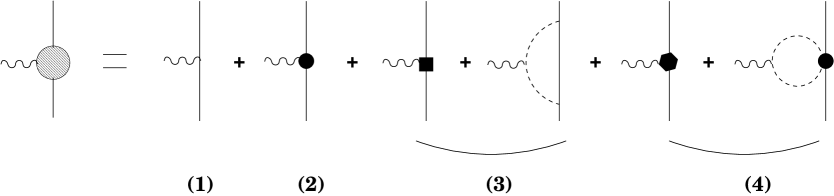
Figure 1: Chiral expansion of a baryon electromagnetic form factor. The lowest order graph (1) with dimension one insertions only gives the charge of the baryon. Tree graphs with insertions from the dimension two (2), three (3) and four (4) effective Lagrangian are depicted by the solid circle, square and sextangle, in order. Pion loop graphs start at third order (3), and fourth order loop graphs (4) have exactly one dimension two insertion. Only one typical loop graph at the orders considered is shown. Solid, dashed and wiggly lines denote baryons, pions and photons, respectively.

For practitioners in chiral EFTs the points discussed in this section are common knowledge. In fact, the vast majority of processes calculated in HBCHPT at the one-loop level (e.g. $\pi N\to\pi N,\;\pi N\rightarrow\pi\pi N,\;\gamma N\rightarrow\pi N,\;\gamma^{\ast}N\to\pi N,\ldots$) behave completely analogous to the scenario displayed in Eq.(1) for the isovector Dirac radius. In such type of scenarios dimensional regularization is the effective method of choice, all symmetries of the theory are automatically preserved and the entire information (up to a given order in the perturbative calculation) on short and long distance physics is contained in the result, independent of the particular regularization scale chosen. However, there are some one-loop calculations that at first sight appear to generate a scale–independent result. The question arises how the discussion given here translates to these special cases where only polynomial divergences appear in the calculation of the loop integrals. These polynomial divergences are automatically eaten up in dimensional regularization, providing us with a nice, seemingly scale-free one–loop prediction. The most prominent example, the leading-one-loop pion contribution to the mass of the nucleon, is discussed in the next section.

3 A comparison of dimensional and cutoff regularization

3.1 Third order calculation of the nucleon mass in dimensional regularization

The leading one–loop calculation of the mass of the nucleon in HBCHPT gives

$$M_{N}^{(3)} = M_{0}-4\,c_{1}m_{\pi}^{2}-\frac{3\,g_{A}^{2}}{32\pi F_{\pi}^{2}}\,m_{\pi}^{3}+{\cal O}(p^{4})\;.$$ (3)

Here, $p$ denotes a small parameter (external momentum, meson mass) and $M_{0}$ corresponds to the nucleon mass in the chiral limit. Its precise value is not well known. Various analyses [26, 27, 28, 29] suggest values in the range $0.75\ldots 0.9$ GeV. It is hoped that new lattice analysis will provide a better understanding of this important nucleon structure parameter [30]. Similarly, $g_{A}$ and $F_{\pi}$ should be taken at their values in the chiral limit, but for our arguments this fine point is of no relevance (as the differences only show up at higher orders). $c_{1}$ denotes a dimension two coupling in the chiral Lagrangian sensitive to the internal structure of the nucleon in close connection to the pion–nucleon sigma term. Most determinations agree about its sign but are uncertain about its precise value (related to the still unsatisfactory situation in the extraction of the pion-nucleon sigma term based on various partial waves analyses of elastic $\pi$N scattering data): $c_{1}=-0.9\pm 0.5$ GeV^-1 [31, 32, 33, 34, 35, 36, 37]. Choosing the central value for $c_{1}$ and fixing $M_{0}=0.88$ GeV to reproduce the physical mass of the nucleon for $m_{\pi}=0.138$ GeV one therefore obtains the mass of the nucleon as a function of the mass of the pion as shown in Fig. 2. Since the result for the one-loop mass shift is finite, the only dimensionfull scale in the problem is the pion mass. The term proportional to a fractional power of the quark masses is generic to the chiral expansion of the octet baryon masses in terms of pion, eta and kaon Goldstone bosons. In lattice gauge studies one usually has to deal with rather large pion masses and thus is interested in a theoretically well-founded extrapolation function to obtain a prediction for an observable at the physical pion mass. From Fig. 2 one clearly sees that Eq. (3) is only able to give a sensible description of the nucleon mass may be out to pion masses of 400 MeV. In the next section we will demonstrate that this breakdown of the leading one-loop HBCHPT result for Goldstone boson masses in this range is connected with the rise of short distance physics contributions, which are not properly controlled in standard dimensional regularization for $m_{\pi}>400$ MeV. Without giving any details we just note that the addition of explicit $\Delta$(1232) degrees of freedom in the non-relativistic SSE scheme does not dramatically improve this situation.

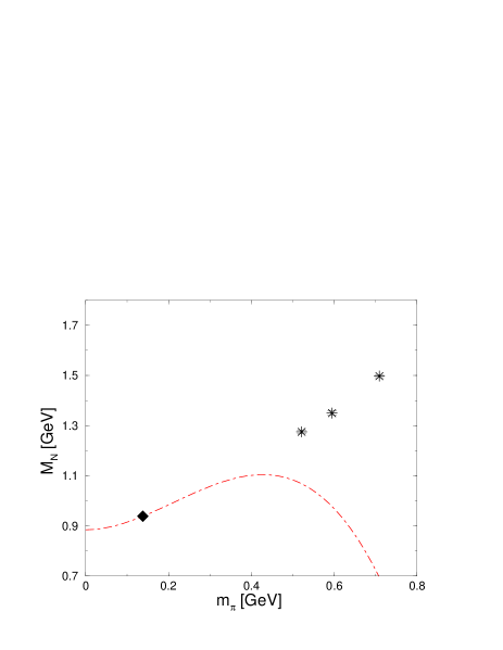
Figure 2: Mass of the nucleon calculated to ${\cal O}(p^{3})$ in HBCHPT plotted as a function of the mass of the pion. The parameter choices made are discussed in the text. One can clearly see that this simple leading one-loop calculation breaks down around $m_{\pi}=400$ MeV. The lattice data (stars) shown have been selected from Ref. [10, 38]. The filled diamond gives the nucleon mass at the physical value of the pion mass.

While Fig. 2 might be a disappointment to any QCD lattice practitioner who would like to extrapolate large quark mass simulations of the nucleon mass down to the physical point utilizing Eq.(3), from the point of view of CHPT such a behaviour is entirely consistent and in some sense even expected. It would be entirely unreasonable to assume that this leading non-analytic pion mass dependence calculated at the leading-one-loop level in HBCHPT should be enough to describe quark-mass dependent physics far above the physical pion mass, as witnessed by the fact that there are large fourth order corrections to the baryon masses. In the present context we now want to study the question whether the same leading one–loop ${\cal O}(p^{3})$ calculation of the same diagram miraculously can give a much better behaved result for large pion masses when the calculation is performed with the help of a cutoff regularization procedure instead of the so-far employed dimensional regularization. This might at first sound strange to any practitioner of field theory, but in the context of an underlying power counting a different regularization scheme might lead to a reordering of the expansion and thus improve the convergence.

3.2 Third order calculation of the nucleon mass in cutoff regularization

Evaluating the same diagrams as before with the help of a radial cutoff $\Lambda$ one obtains the following finite expression in HBCHPT :

$$M_{N}^{(3)} = M_{0}^{(r)}-4c_{1}^{(r)}\,m_{\pi}^{2}-\frac{3\,g_{A}^{2}}{32\pi F_{\pi}^{2}}\,m_{\pi}^{3}+\frac{3\,g_{A}^{2}}{(4\pi F_{\pi})^{2}}\,m_{\pi}^{3}\arctan\frac{m_{\pi}}{\Lambda}$$ (4)

with

$$M_{0}^{(r)} = M_{0}-\frac{g_{A}^{2}}{(4\pi F_{\pi})^{2}}\,\Lambda^{3}\,,$$

$$c_{1}^{(r)} = c_{1}-\frac{3\,g_{A}^{2}}{4(4\pi F_{\pi})^{2}}\,\Lambda\,.$$ (5)

Having absorbed the polynomial divergences in $\Lambda$ into the coefficients $M_{0}$ and $c_{1}$, we have regulated the high-energy behaviour and obtained a finite result. Note that in dimensional regularization, the parameters at dimension one and two of the effective Lagrangian do not get renormalized. However, one should keep in mind that the effective field theory is only defined for momenta $p\leq\Lambda_{\chi}\approx 1$ GeV. For $\Lambda\geq\Lambda_{\chi}$ we must therefore be able to map the residual cutoff dependence onto a string of higher order couplings that are suppressed by inverse powers of $\Lambda_{\chi}$. One finds

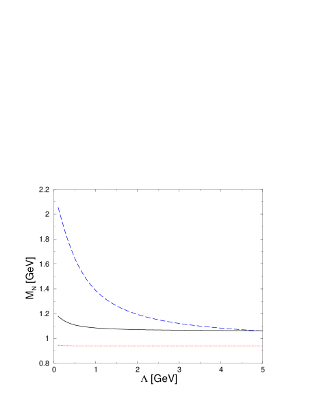
Figure 3: Cutoff dependence of the nucleon mass calculated at ${\mathcal{O}}(p^{3})$ in HBCHPT. The dotted, solid and dashed curve correspond to a pion mass of 140, 300 and 600 MeV, in order. No plateau is found in the region of applicability of CHPT (i.e. for $\Lambda<1$ GeV) for $m_{\pi}>400\,$MeV.

$$M_{N}^{(3)} = M_{0}^{(r)}-4\,c_{1}^{(r)}\,m_{\pi}^{2}-\frac{3\,g_{A}^{2}}{32\pi F_{\pi}^{2}}\,m_{\pi}^{3}+\frac{3\,g_{A}^{2}}{(4\pi F_{\pi})^{2}}\,m_{\pi}^{3}\left\{\frac{m_{\pi}}{\Lambda_{\chi}}-\frac{1}{3}\,\left(\frac{m_{\pi}}{\Lambda_{\chi}}\right)^{3}+\ldots\right\}$$ (6)

$$= M_{0}^{(r)}-4\,c_{1}^{(r)}m_{\pi}^{2}-\frac{3\,g_{A}^{2}}{32\pi F_{\pi}^{2}}\,m_{\pi}^{3}+{\cal O}(p^{4})\;.$$

To third order ${\cal O}(p^{3})$ one therefore obtains exactly the same result in cutoff and in dimensional regularization, as expected (for a related discussion between dimensionally and cutoff regularized loop integrals in chiral nuclear EFT, see [41]). We note that the terms beyond the ${\cal O}(p^{3})$ truncation only contain even powers of $m_{\pi}$, showing that the cutoff scheme employed here respects chiral symmetry at the one–loop level, since such terms are analytic in the quark masses and can thus be absorbed in the polynomial terms generated by the effective Lagrangian. We note that most of the regulating functions for one-loop diagrams proposed in [9] do not share this property, but generate e.g. terms $\sim m_{\pi}^{5}/\Lambda_{\chi}^{2}$, which can only be mapped onto a systematic chiral expansion at the two-loop level. In conclusion we note that formally the correspondence between the results obtained in dimensional and cutoff regularization is obtained by an expansion of the cutoff result in powers of $1/\Lambda=1/\Lambda_{\chi}$.

In Fig. 3 we now show the resulting cutoff dependence of the nucleon mass to leading one-loop order in HBCHPT of Eq.(4) for various values of the pion mass. As expected, for the physical value of $m_{\pi}$, we have a nice plateau for all cutoff values below $\Lambda_{\chi}$, clearly showing that CHPT for two flavors is well behaved. For $m_{\pi}=300$ one observes already some curvature in the range of reasonable cutoffs, whereas for a pion mass as large as 600 MeV, there is no stable prediction in the range of physically allowed cutoffs. We therefore observe that the breakdown of the leading one-loop HBCHPT result of dimensional regularization as seen in Fig. 2 and the disappearance of a stable plateau in the low energy region in the cutoff approach, cf. Fig. 3, occur in the same mass range. Both phenomena point to the fact that for Goldstone Boson masses larger than 400 MeV the standard counting of CHPT has be modified to properly account for the short distance physics. In the next section we will present such a modification within the cutoff approach.

3.3 Introduction of an improvement term

The expansion of the nucleon mass using cutoff regularization given in Eq. (6) allows us to propose an improvement scheme to avoid the strong cutoff dependence for larger pion masses exhibited in Fig. 3. This can be done entirely within the operator structure of the EFT under consideration and without resorting to phenomenological and model–dependent methods like additional form factors, with a cutoff scale possibly inspired by the scale set by the hadron size. Clearly, the improvement term we are after has to fulfill two requirements: First, it must lead to the same structure as the leading $1/\Lambda$ correction in Eq. (6) and, second, must allow us to cancel the strong cutoff sensitivity induced by this term. In fact, the corresponding term appears in the chiral pion–nucleon Lagrangian at fourth order as combination of three operators. Following the notation of Ref. [42] these read

$${\cal L}_{\pi N}^{(4)}=e_{38}\,\bar{\psi}\,\langle\chi_{+}\rangle^{2}\,\psi+e_{115}\,\bar{\psi}\,\frac{1}{4}\langle\chi_{+}^{2}-\chi_{-}^{2}\rangle\,\psi-e_{116}\,\bar{\psi}\,\frac{1}{4}\biggl{(}\langle\chi_{-}^{2}\rangle-\langle\chi_{-}\rangle^{2}+\langle\chi_{+}^{2}\rangle-\langle\chi_{+}\rangle^{2}\biggr{)}\,\psi~{},$$ (7)

where $\psi$ denotes the nucleon field and $\chi_{\pm}$ parametrizes the explicit chiral symmetry breaking through the quark masses (for precise definitions, see [42]). These three terms combine to give one operator without pion fields,

$${\cal L}_{\pi N}^{(4)}=4e_{1}\,\bar{\psi}\,m_{\pi}^{4}\,\psi~{},$$ (8)

with $e_{1}=16e_{38}+2e_{115}+e_{116}/2$. Furthermore, the LEC $e_{1}$ can be written in terms of a finite term and a second contribution that cancels the leading $1/\Lambda$ correction in Eq. (6), specifically

$$e_{1}=e_{1}^{\rm fin}-\frac{3g_{A}^{2}}{16\pi^{2}F_{\pi}^{2}}\,\frac{1}{\Lambda}~{}.$$ (9)

Note the minus sign in front of the second term in this equation, it follows from the requirement that the leading $1/\Lambda$ correction should be canceled. Although formally of higher order, one should consider such a term as being promoted to the order one is working (that is to an order below its formal appearance) if one insists on a cutoff–independent result.

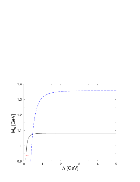
Figure 4: Cutoff dependence of the nucleon mass calculated at ${\mathcal{O}}(p^{3})$ in HBCHPT employing the improvement scheme. The dotted, solid and dashed curve correspond to a pion mass of 140, 300 and 600 MeV, in order. A plateau in the region of applicability of CHPT (i.e. for $\Lambda<1$ GeV) can now be found for Goldstone boson masses up to $300\,$MeV.

To show the effect of adding this improvement term, we display in Fig. 4 the cutoff dependence of the nucleon mass calculated to third order supplemented with the improvement term Eq. (9) and setting the finite piece to zero, $e_{1}^{\rm fin}=0$, for simplicity. For the physical value of the pion mass, the plateau is, of course, not affected. However, we now also observe a nice plateau for cutoff values between 400 MeV and $\Lambda_{\chi}$ for the larger pion mass $m_{\pi}=300\,$MeV. For the even larger pion mass of about 600 MeV, this simple procedure is still not sufficient to lead to a plateau at sufficiently low values of the cutoff, but compared to the calculation shown in Fig. 3 we notice a much less pronounced cutoff sensitivity. As a consequence, one can also trust the quark mass expansion of the nucleon mass to higher pion masses as shown in Fig. 5. Here, we have adjusted $e_{1}^{\rm fin}$ such as to have the correct mass of the nucleon for the physical value of the pion mass. It is clear from that figure that the third order contribution is now reduced compared to the result based on dimensional regularization, however, one still has to be careful in applying this improved form at too large pion masses, simply because the term linear in the quark masses becomes very large for pion masses above 500 MeV.

Clearly, this procedure should be considered as the minimal method to improve calculations in cutoff schemes. We stress again that all operators required to achieve such an improvement are part of the effective Lagrangian under consideration and thus automatically chiral symmetry and the pertinent Ward identities are respected. It is also important to stress that such an improvement does not come for free - one has to include one more higher order operator with a tunable finite coefficient, e.g. in the example just discussed, one would adjust $e_{1}^{\rm fin}$ so as to reproduce the physical nucleon mass for the cutoff under consideration (as it was done for example to generate Fig. 5). From the purists point of view, this procedure is of course not entirely satisfactory since there are other terms at the same order as the improvement term which should eventually be considered. However, our ambition is more modest, we simply want to set up a simple scheme within the EFT to reduce the possible cutoff dependence in such schemes. Note that similar methods are also used in pionless nuclear effective field theory approaches to few–nucleon systems, see e.g. [43, 44]. In the appendix, we briefly discuss the third order result for the nucleon isovector anomalous magnetic moment employing dimensional and (improved) cutoff regularization.

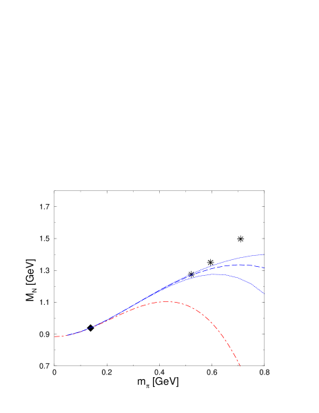
Figure 5: Nucleon mass calculated to third order in HBCHPT as a function of the pion mass. The solid curve shows the ${\mathcal{O}}(\Lambda^{-1}$) improved scheme, whereas the dotted curve shows the result in standard dimensional regularization. The solid line refers to a cutoff $\Lambda=1\,$GeV, whereas the dotted lines give the corresponding results for $\Lambda=0.8\,$GeV and $\Lambda=1.2\,$GeV, respectively. For further notation see Fig. 2

We now proceed to analyze the nucleon mass to fourth order in the chiral expansion, that is to second order in the quark masses. It is a well established fact from many studies of Goldstone boson effects in baryon masses that such effects can not be neglected, see e.g. [12, 28]. Of course, in these studies, large Goldstone boson loops are generated from intermediate kaons and etas whereas we are considering the case of increasing the pion mass within two–flavor QCD. Apart from group structure complications, these two cases are equivalent.

4 Nucleon mass to fourth order and chiral extrapolation

In this section, we discuss the nucleon mass shift to fourth order in the chiral expansion and how it can be used (or misused) to perform chiral extrapolations for lattice gauge theory results obtained at much larger pion masses than the physical value. We stress that even the improved one–loop representations discussed here should not be used at pion masses above $600\ldots 700$ MeV, since one then is too close to the breakdown scale of the chiral expansion. Still, for purely illustrative purpose, we will apply our formalism to lattice results for pion masses ranging from 500 MeV to 800 MeV.

4.1 Fourth order calculation of the nucleon mass

As was derived in [45] the fourth order mass shift for a nucleon with four–velocity $v_{\mu}$ and residual momentum $k_{\mu}$ is given by:

$$M^{(4)}=i\,\left(\Sigma^{(4)}(\omega=0)-4c_{1}m_{\pi}^{2}\Sigma^{\prime(3)}(\omega=0)\right)~{},$$ (10)

where $\omega=v\cdot k$, $\Sigma^{(4)}(\omega)$ is the self–energy to fourth order and $\Sigma^{\prime(3)}(\omega)$ the derivative with respect to $\omega$ of the self–energy to third order. In dimensional regularization, the nucleon mass to fourth order takes the form [45]

$$M_{N}^{(4)} = M_{0}-4\,c_{1}m_{\pi}^{2}-\frac{3\,g_{A}^{2}}{32\pi F_{\pi}^{2}}\,m_{\pi}^{3}-4\,e_{1}(\lambda)m_{\pi}^{4}+\frac{3}{128\pi^{2}F_{\pi}^{2}}\left(c_{2}-\frac{2g_{A}^{2}}{M_{N}}\right)\,m_{\pi}^{4}$$ (11)

$$\qquad-\frac{3}{32\pi^{2}F_{\pi}^{2}}\,\left(-8c_{1}+c_{2}+4c_{3}+\frac{g_{A}^{2}}{M_{N}}\right)\,m_{\pi}^{4}\,\ln\frac{m_{\pi}}{\lambda}+{\cal O}(p^{5})\;,$$

where $e_{1}(\lambda)$ is a combination of LECs from the fourth order chiral Lagrangian, as discussed earlier. As shown below, the numerical value of this LEC is not well known, so for a first orientation we will vary this LEC in the range from $-1$ to $1$ (in units of GeV^-3), which are values of natural size, always setting $\lambda=1\,$GeV. That, however, is a very conservative estimate and we will later at least fix the sign of $e_{1}$. For the present discussion, it is, however, instructive to work with the full range consistent with naturalness. The dimension two LECs $c_{2},c_{3}$ are known to some accuracy, the precise values we use will be given later. Note also that fifth order corrections to Eq. (11) have been worked out [46] and found to be extremely small for the physical value of $m_{\pi}$ and, furthermore, these $1/M_{N}$ corrections are given parameter–free. Shifting now to cut-off regularization, one obtains for the fourth order contribution to the nucleon mass

$$\delta M_{N}^{(4)} = -{\frac{3}{32\pi^{2}M_{N}F_{\pi}^{2}}}\biggl{\{}\frac{1}{{3\sqrt{1+m_{\pi}^{2}/\Lambda^{2}}}}\bigl{[}\Lambda^{4}(1-\sqrt{1+m_{\pi}^{2}/\Lambda^{2}})(g_{A}^{2}-2M_{N}(c_{2}+4c_{3}))$$ (12)

$$+m_{\pi}^{2}\Lambda^{2}(g_{A}^{2}(1-\frac{1}{2}\sqrt{1+m_{\pi}^{2}/\Lambda^{2}})+M_{N}(c_{2}+4c_{3})(1-2\sqrt{1+m_{\pi}^{2}/\Lambda^{2}})$$

$$-24M_{N}c_{1}(1-\sqrt{1+m_{\pi}^{2}/\Lambda^{2}}))+3m_{\pi}^{4}(g_{A}^{2}+M_{N}(c_{2}+4c_{3}-8c_{1}))\bigr{]}$$

$$+(g_{A}^{2}-M_{N}(8c_{1}-c_{2}-4c_{3}))m_{\pi}^{4}\,\biggl{[}\ln\frac{m_{\pi}}{M_{0}}-\ln\frac{1}{2}\biggl{(}1+\sqrt{1+\frac{m_{\pi}^{2}}{\Lambda^{2}}}\biggr{)}\biggr{]}\biggl{\}}-4e_{1}^{(r)}\,m_{\pi}^{4}~{},$$

with a further renormalization of the constants $M_{0}^{(r)}$ and $c_{1}^{(r)}$ of Eq. (3.2),

$$M_{0}^{(r)} = -{\frac{1}{32\pi^{2}M_{N}F_{\pi}^{2}}}\Lambda^{4}\left(g_{A}^{2}-2M_{N}(c_{2}+4c_{3})\right)~{},$$

$$c_{1}^{(r)} = -{\frac{1}{64\pi^{2}M_{N}F_{\pi}^{2}}}m_{\pi}^{2}\Lambda^{2}\left(g_{A}^{2}+M_{N}(-48c_{1}+4c_{2}+16c_{3})\right)~{},$$ (13)

and an additional renormalization of the LEC $e_{1}$,

$$e_{1}^{(r)}=e_{1}+\frac{3}{128\pi^{2}M_{N}F_{\pi}^{2}}\bigl{(}g_{A}^{2}-M_{N}(8c_{1}-c_{2}-4c_{3})\bigr{)}\,\ln\frac{\Lambda}{M_{0}}~{}.$$ (14)

As before, having absorbed the polynomial as well as the logarithmic divergences in $\Lambda$ into the coefficients $M_{0}$, $c_{1}$ and $e_{1}$, we have regulated the high-energy behaviour and obtained a finite result. We note that the fourth order contribution $\delta M^{(4)}$ is given by a polynomial in even powers of $m_{\pi}$ plus a non–analytic piece. This last one is exactly the same as obtained in dimensional regularization and thus the cut-off scheme preserves chiral symmetry up to fourth order. In contrast to the third order case discussed earlier, one observes a very weak cutoff dependence of the nucleon mass as $m_{\pi}$ increases as long as $m_{\pi}\leq 400\,$MeV, as shown in Fig. 6. If one also wants to obtain a plateau for larger pion masses below the chiral symmetry breaking scale, one proceeds in the same way as done before, namely by adding a six order counterterm such that it has a contribution that cancels the leading $1/\Lambda^{2}$ correction:

$$\delta M^{(4)}_{\rm imp}=\delta M^{(4)}+dm_{\pi}^{6}~{},$$ (15)

with

$$d=d^{\rm{fin}}-{\frac{5}{512\pi^{2}M_{N}F_{\pi}^{2}\Lambda^{2}}}\biggl{(}7g_{A}^{2}-4M_{N}\bigl{(}{\frac{36}{5}}c_{1}-c_{2}-4c_{3}\bigr{)}\biggr{)}~{}.$$ (16)

As before, the so improved result shows a much weaker cut–off dependence.

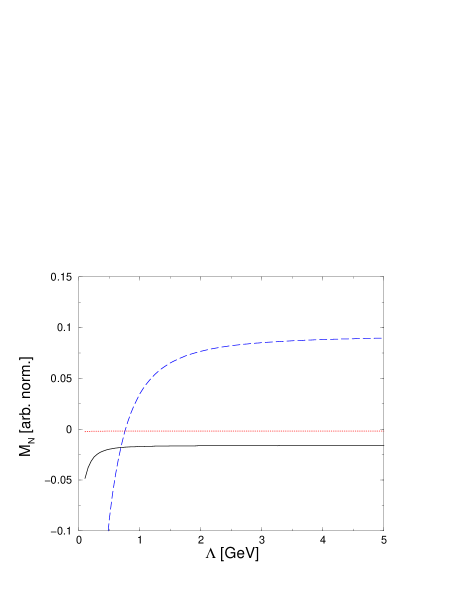
Figure 6: Cutoff dependence of the nucleon mass calculated at ${\mathcal{O}}(p^{4})$ in HBCHPT employing cutoff regularization with $\Lambda=1\,$GeV (in arbitrary normalization). For notation, see Fig. 3.

4.2 Numerical results and chiral extrapolation

For discussing the numerical results, we have to give the values of the LECs appearing in the chiral expansion. We use here $c_{1}=-0.9\,$GeV^-1, $c_{2}=3.2\,$GeV^-1 and $c_{3}=-5.7\,$GeV^-1 (and also some smaller (in magnitude) values for $c_{3}$ as discussed below), see e.g. [32]. The pion mass dependence of the nucleon mass to fourth order is shown in Fig. 7. We see that for pion masses below 400 MeV, the fourth order correction is fairly small, for the physical value of $m_{\pi}$ these fourth order corrections are so small that they can safely be neglected. For larger values of $m_{\pi}$, the uncertainty due to the variation in $e_{1}(\lambda)$ becomes quickly very large. This clearly shows that it is very dangerous to use a formula like Eq. (11) for too large pion masses if one has no means to pin down the LEC $e_{1}$ with some accuracy. Fortunately, from the analysis of pion–nucleon scattering to fourth order we know that $e_{1}$ should be of order 1 GeV^-3 and negative [35]. We note that there is some cancellation between the $m_{\pi}\ln m_{\pi}$ and the $m_{\pi}$ contributions in $\delta M^{(4)}$ for negative values of $e_{1}$. If one e.g. changes the value of the $c_{3}$ to $-4\,$GeV^-1, the nucleon mass increases monotonically with increasing pion mass, as shown by the dotted line in Fig. 7, a trend consistent with recent lattice data [38]

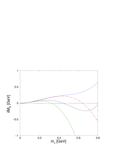
Figure 7: Pion mass dependence of the nucleon mass shift $\delta M_{N}=\delta M_{N}^{(2)}+\delta M_{N}^{(3)}+\delta M_{N}^{(4)}$. The dot–dashed line gives the third order mass shift, whereas the fourth order shift is given by the solid and dashed lines for $e_{1}=1$ and $e_{1}=-1$, respectively. The dotted line gives the fourth order result using $e_{1}=-1$ and $c_{3}=-4$ (in appropriate units of inverse GeV).

In Fig. 8 (left panel) we show the pion mass dependence of the nucleon mass based on the dimensional regularization and allowing for variation in the LEC $c_{3}$ to fit the lattice “data” from the CP-PACS collaboration [38]. We use $c_{3}=-3.45\,\rm GeV^{-1}$, $e_{1}=-1\,\rm GeV^{-3}$, and all other parameters and LECs as stated before. Note that for $g_{A}$ and $F_{\pi}$, we use the physical values. One could also use the corresponding values in the chiral limit, which only leads to a small change in the fit value for $c_{3}$, as we have convinced ourselves. It is rather obvious that contrary to statements made in the literature, the fourth order representation employing dimensional regularization can describe the quark mass dependence of the lattice results without any need of unnatural values for any of the LECs  or the inclusion of higher order terms not generated in a symmetry–preserving one–loop calculation. It should, however, be stressed again that for pion masses above 600 MeV the fourth order corrections become unpleasantly large. In the right panel of Fig. 8, we show the results employing cutoff regularization (with the third order result including the improvement term as discussed earlier). Again, the trend of the lattice results is nicely reproduced setting $c_{3}=-3.9\,\rm GeV^{-1}$ and $e_{1}=-0.75\,\rm GeV^{-3}$, which are modest changes to the values used in the case of dimensional regularization. Furthermore, these values are within uncertainties consistent with extractions from pion–nucleon scattering. Note that the corrections going from third to fourth order are sizeably smaller than in case of dimensional regularization, which is mostly due to the improvement term included in the third order result. We point out again that in contrast to statements found in the literature, these one–loop cutoff representations are quite capable of describing the pion mass dependence of the nucleon mass found in lattice gauge theory calculations. The dependence on the actual choice of the cut–off $\Lambda$ is also shown in the right panel of Fig. 8, where the dotted line refers to the fourth order result with $\Lambda=1.2\,$GeV. For the expression based on dimensional regularization to work above 600 MeV, one has to include the sixth order term as in the improved cut–off scheme. We stress again that applying the one–loop expressions to pion masses above 600 MeV is only done for illustrative purposes, for a realistic chiral extrapolation smaller pion masses are mandatory. For a more detailed study of nucleon mass chiral extrapolations based on such and similar regularizations, see [47].

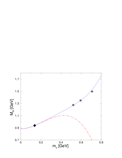
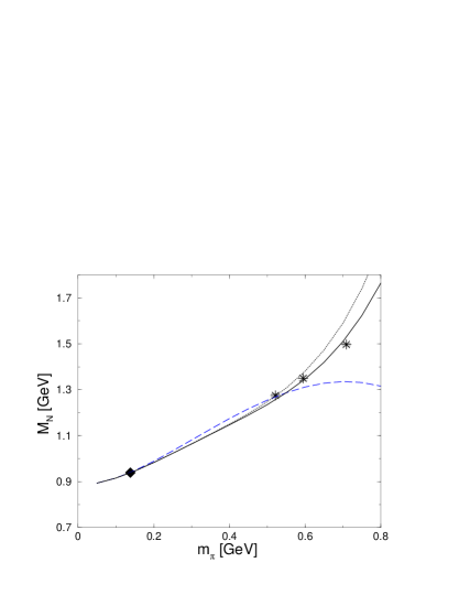
Figure 8: Chiral extrapolation of the nucleon mass. Left panel: best fit to the CP-PACS lattice results [38] employing dimensional regularization. The dot–dashed line refers to the parameter–free third order result whereas the dotted line gives the fit based on the fourth order representation for the values of the LECs given in the text. Right panel: Best fit in cutoff regularization. The dashed line gives the improved third order result with one adjusted parameter. The solid (dotted) line refers to the fit based on the fourth order representation for the values of the LECs given in the text with $\Lambda=1\,(1.2)\,$GeV.

To further sharpen these statements, it is constructive to consider the convergence of the chiral expansion for the nucleon mass as the pion mass is increased. In Table 1 we have collected the pertinent results. Consider first dimensional regularization. As it is well known and has been stressed before, for the physical value of the pion mass the convergence is excellent, and it is even fairly good for $m_{\pi}=300\,$MeV. Only for the large mass of 600 MeV, one has sizeable cancellations between the second and third order pieces accompanied with a non–negligible fourth order contribution. This is very reminiscent of the chiral expansion of the ground state octet masses in terms of kaon and eta loop contributions. In cutoff regularization. the convergence properties are very visibly improved, so that even at $m_{\pi}=600\,$MeV the series is fairly well behaved.

		Dim. Reg.		Cutoff
$m_{\pi}$ [GeV]	${\mathcal{O}}(q^{2}$)	${\mathcal{O}}(q^{3}$)	${\mathcal{O}}(q^{4})$	${\mathcal{O}}(q^{3}$)	${\mathcal{O}}(q^{4})$
$0.138$	0.069	$-$0.015	$-$0.0007	$-$0.014	$-$0.002
$0.300$	0.32	$-$0.151	0.014	$-$0.128	$-$0.017
$0.600$	1.30	$-$1.212	0.386	$-$0.869	0.034

Table 1: Convergence of the chiral series for the nucleon mass employing dimensional and cutoff regularization. The various contributions are given in GeV.

5 Criteria for a stable cutoff scheme

Based on the example discussed above, we can set up a general checklist for a consistent cutoff regularization procedure. It consists of the following steps:

Step 1: Choose a cutoff scheme and calculate all diagrams to the desired chiral order in that scheme.

Step 2: Absorb all polynomial ($\sim\Lambda^{n}$) and logarithmic ($\sim\ln\Lambda$) divergences appearing to that order in counter terms. The finite (scale–dependent) parts of the corresponding LECs have to be kept as part of the full result, even when nothing is known about their size.

Step 3: Perform the chiral symmetry check: Expand the finite result in a series in inverse powers of the cutoff $\sim\Lambda^{-n}$ and check if the associated quark mass dependence is analytic, i.e. one must be able to show that all resulting terms can be matched onto an allowed contact interaction (counter term). If this is not the case, choose a different cutoff scheme or introduce extra terms (see e.g. [48]) to correct for chiral symmetry violation.

Step 4: In case that the constraints from chiral symmetry are fulfilled, study the scale dependence of the full (unexpanded) finite result as a function of the cutoff scale. Look for the onset of the plateau. If the plateau is reached for values $\Lambda<\Lambda_{\chi}$ the calculation is consistent.

Step 5: If no plateau is found within the region of validity of the chiral effective field theory improvement terms must be added. The (negative of the) leading term in the Taylor expansion in the cutoff scale discussed in step 3 provides the scale dependence for the local improvement term. The corresponding operator structure of the improvement term can also be read off from the Taylor expansion. As this term is analytic in the quark mass and allowed by chiral symmetry, the existence of this operator as part of a chiral Lagrangian is guaranteed.

Step 6: Add the improvement term to the unexpanded finite result. Note that this improvement term also carries a finite part of unknown strength, as there is no free lunch in this world (or in other words: You cannot fool QCD into a reduced number of possible short distance operators, this only works in models). Analyze the remaining scale dependence: if the plateau now begins for cutoff values below the breakdown scale of the theory the addition of one improvement term was sufficient. If that is not the case, go back to step 5 and continue the procedure until a satisfactory result is obtained.

This concludes our list to obtain stable prediction using cutoff regularization.

6 Summary and conclusions

We summarize the main results of our work:

• CHPT results for the baryon structure always depend on an interplay between long and short distance physics. The relative strength between these two sectors depends in general on the regularization scale chosen. Only the sum of the two contributions gives a scale–independent result. This statement holds independent of the regularization scheme (cutoff, dimensional regularization, $\ldots$) chosen.

• As soon as one goes beyond a leading order tree level analysis, the internal structure of hadrons is build up in CHPT. Two mechanism contribute to the internal structure effects: higher dimensional operators consistent with chiral symmetry and quantum fluctuations associated with Goldstone boson effects. This “finite size” of the nucleon emerges in chiral EFTs irrespective of the regularization scheme chosen.

• Cutoff schemes are legitimate regularization procedures in CHPT (or other chiral EFTs), provided that one checks carefully that terms generated by the employed scheme which are in conflict with chiral symmetry have all been removed. In section 5 we have proposed test criteria which indicate whether the cutoff scheme chosen is appropriate for the question under study.

• If a cutoff procedure fails the test criteria specified in section 5, improvement terms have to be added in the Lagrangian where the problem (i.e. large scale dependence in the region of validity of the theory) occurs. In section 3.3 we have shown how such an $O(\Lambda^{-1})$ improvement term may look like for the simple example of the nucleon mass to leading one–loop order in HBCHPT. Given that such improvement terms can be generated within the CHPT framework, we see no necessity to resort to phenomenologically inspired regularization procedure (e.g. inserting an exponential suppression factor into the chiral loop integrals “by hand”). If the unimproved cutoff result has been properly corrected for any chiral symmetry breaking terms, then the addition of the improvement term calculated from this result also automatically fulfills all the constraints of chiral symmetry. In particular, it will not violate any strictures arising from (chiral) Ward identities, which is not guaranteed when adding phenomenologically inspired regulators to chiral loop integrals.

• Comparisons between (scale–dependent) pion loop results obtained in CHPT (or any variant thereof) and phenomenological models are difficult. Qualitative comparisons to results obtained via dimensional regularization can only be obtained for “small” values of $\lambda\leq 600$ MeV, where $\lambda$ is the scale of dimensional regularization.

• For the large majority of one-loop results in CHPT we see no need to give up dimensional regularization as the tool of choice, as the results in their interplay between short and long distance physics properly account for the internal (finite size) structure of the nucleon, e.g. see Eq. (1). This statement holds independent of the masses of the Goldstone bosons involved, e.g. also for “heavy” pions in lattice simulations or octet Goldstone bosons. However, we note that cutoff approaches can be particularly useful in those special cases where the leading one–loop result obtained in dimensional regularization appears to be scale-independent and at the same time the mass of the involved Goldstone boson is large. We note that the improvement procedures outline here can lead to a revived analysis of SU(3) chiral dynamics, where for example the baryon mass calculation is exactly plagued by these problems.

• We have analyzed the quark mass expansion of the nucleon mass to second order in the quark masses in dimensional as well as in cutoff regularization. This representation can be used successfully to describe lattice data obtained for pion masses between 500 and 750 MeV, although for theoretical reasons such a chiral extrapolation should at most be trusted up to masses of about 600 MeV. Our results clearly rule out statements found in the literature that one needs terms of very high orders to construct a sensible chiral extrapolation function, furthermore, in our calculation chiral symmetry is preserved at each step. Although these findings are promising, we urge the lattice practitioners to generate results for pion masses below 500 MeV to really make contact to the chiral properties of QCD.

Appendix A Third order calculation of the nucleon isovector anomalous magnetic moment

Here, we wish to discuss the isovector anomalous magnetic moment of the nucleon, because it is also given to leading one–loop order by a simple formula but shows a somewhat different behaviour than the nucleon mass. In dimensional regularization, one has

$$\kappa_{V}=c_{6}-\frac{g_{A}^{2}M_{N}\,m_{\pi}}{4\pi F_{\pi}^{2}}~{},$$ (A.1)

where the LEC $c_{6}$ can be adjusted so as to reproduce the physical value of the isovector anomalous magnetic moment, $\kappa_{V}=3.706$. This leads to $c_{6}=5.62$, which seems unnaturally large but can be understood in terms of resonance saturation [32]. Clearly, the third order result can only be used for pion masses below 400 MeV, because for such a value the loop contribution completely cancels the leading dimension two term $\sim c_{6}$. In fact, to third order the quark mass dependence of $\kappa_{V}$ is rather trivial, the isovector magnetic moment simlpy decreases linearly with increasing $m_{\pi}$. As before, we now want to use a cutoff instead of dimensional regularization. Using again a three–dimensional cutoff, we find

$$\kappa_{V}=c_{6}^{(r)}-{\frac{g_{A}^{2}m_{\pi}M_{N}}{4\pi F_{\pi}^{2}}}+{\frac{g_{A}^{2}M_{N}}{2\pi^{2}F_{\pi}^{2}}}\left(m_{\pi}\arctan{\frac{m_{\pi}}{\Lambda}}+{\frac{1}{3}}{\frac{\Lambda m_{\pi}^{2}}{\Lambda^{2}+m_{\pi}^{2}}}\right)$$ (A.2)

with

$$c_{6}^{(r)}=c_{6}+{\frac{g_{A}^{2}M_{N}}{3\pi^{2}F_{\pi}^{2}}}\Lambda~{}.$$ (A.3)

We note that cutoff dependence is significantly different from the case of the nucleon mass because of the appearance of terms linear in $m_{\pi}/\Lambda$. This is shown in Fig. 9, where even for the physical values of the pion mass we do not find a plateau for cutoff values below the chiral symmetry breaking scale (solid line, for simplicity we have set $c_{6}=0$). Needless to say that this cutoff dependence is even stronger for larger pion masses.

Figure 9: Cutoff dependence of the isovector nucleon anomalous magnetic moment calculated at ${\mathcal{O}}(p^{3})$ in HBCHPT employing cutoff regularization (with an arbitrary normalization). The result without (with) an improvement term as discussed in the text is shown by the solid (dashed) line.

Expanding Eq. (A.2) in inverse powers of $\Lambda$, one gets:

$$\kappa_{V}=c_{6}^{(r)}-{\frac{g_{A}^{2}m_{\pi}M_{N}}{4\pi F_{\pi}^{2}}}+{\frac{g_{A}^{2}M_{N}}{3\pi^{2}F_{\pi}^{2}}}{\frac{m_{\pi}^{2}}{\Lambda}}\left\{2-{\frac{m_{\pi}^{2}}{\Lambda^{2}}}+\cdots\right\}~{}.$$ (A.4)

From this expression, one can readily deduce the improvement term to be subtracted. Again, the corresponding operator appears in the fourth order pion–nucleon Lagrangian, it is the term $e_{105}\bar{\psi}\langle F_{\mu\nu}^{+}\rangle\,\langle\chi_{+}\rangle$ $\sigma^{\mu\nu}\,\psi\,$ [42]. Subtracting this contribution as before and setting the finite part to zero for simplicity, one obtains the dashed curve in Fig. 9, which exhibits a nice plateau for the relevant values of the cutoff, $2m_{\pi}\leq\Lambda\leq\Lambda_{\chi}$.

References

- [1] S. Weinberg, Physica A 96 (1979) 327.
- [2] J. Gasser and H. Leutwyler, Annals Phys. 158 (1984) 142.
- [3] J. Gasser and H. Leutwyler, Nucl. Phys. B 250 (1985) 465.
- [4] S. Weinberg, Phys. Rev. 166 (1968) 1568.
- [5] S. R. Coleman, J. Wess and B. Zumino, Phys. Rev. 177 (1969) 2239.
- [6] C. G. Callan, S. R. Coleman, J. Wess and B. Zumino, Phys. Rev. 177 (1969) 2247.
- [7] J. F. Donoghue and B. R. Holstein, Phys. Lett. B 436 (1998) 331.
- [8] J. F. Donoghue, B. R. Holstein and B. Borasoy, Phys. Rev. D 59 (1999) 036002.
- [9] R. D. Young, D. B. Leinweber and A. W. Thomas, arXiv:hep-lat/0212031.
- [10] D. B. Leinweber, A. W. Thomas and R. D. Young, arXiv:hep-lat/0302020.
- [11] J. Gasser and A. Zepeda, Nucl. Phys. B 174 (1980) 445.
- [12] J. Gasser, Annals Phys. 136 (1981) 62.
- [13] D. Espriu and J. Matias, Nucl. Phys. B 418 (1994) 494.
- [14] V. Bernard, N. Kaiser and U.-G. Meißner, Int. J. Mod. Phys. E 4 (1995) 193.
- [15] T. R. Hemmert, B. R. Holstein and J. Kambor, J. Phys. G 24 (1998) 1831.
- [16] P. J. Ellis and H. B. Tang, Phys. Rev. C 56 (1997) 3363.
- [17] T. Becher and H. Leutwyler, Eur. Phys. J. C 9 (1999) 643.
- [18] V. Bernard, T. R. Hemmert and U.-G. Meißner, Phys. Lett. B 565 (2002) 137.
- [19] V. Bernard, T. R. Hemmert and U.-G. Meißner, Phys. Lett. B 545 (2002) 105.
- [20] V. Bernard, T. R. Hemmert and U.-G. Meißner, Phys. Rev. D 67 (2003) 076008.
- [21] V. Bernard, N. Kaiser, J. Kambor and U.-G. Meißner, Nucl. Phys. B 388 (1992) 315.
- [22] P. Mergell, U.-G. Meißner and D. Drechsel, Nucl. Phys. A 596 (1996) 367.
- [23] H. W. Hammer, U.-G. Meißner and D. Drechsel, Phys. Lett. B 385 (1996) 343.
- [24] V. Bernard, H.W. Fearing, T.R. Hemmert and U.-G. Meißner, Nucl. Phys. Nucl. Phys. A 635 (1998) 121 [Erratum-ibid. A 642 563].
- [25] B. Kubis and U.-G. Meißner, Nucl. Phys. A 679 (2001) 698.
- [26] J. Gasser, H. Leutwyler and M. E. Sainio, Phys. Lett. B 253 (1991) 260.
- [27] E. Jenkins and A. V. Manohar, Phys. Lett. B 281 (1992) 336.
- [28] B. Borasoy and U.-G. Meißner, Annals Phys. 254 (1997) 192.
- [29] B. Borasoy, Eur. Phys. J. C 8 (1999) 121.
- [30] G. Schierholz et al. (QCDSF collaboration), in preparation.
- [31] V. Bernard, N. Kaiser and U.-G. Meißner, Nucl. Phys. B 457 (1995) 147.
- [32] V. Bernard, N. Kaiser and U.-G. Meißner, Nucl. Phys. A 615 (1997) 483.
- [33] M. Mojžiš, Eur. Phys. J. C 2 (1998) 181.
- [34] N. Fettes, U.-G. Meißner and S. Steininger, Nucl. Phys. A 640 (1998) 199.
- [35] N. Fettes and U.-G. Meißner, Nucl. Phys. A 676 (2000) 311.
- [36] T. Becher and H. Leutwyler, JHEP 0106 (2001) 017.
- [37] K. Torikoshi and P. J. Ellis, Phys. Rev. C 67 (2003) 015208.
- [38] A. Ali Khan et al. [CP-PACS Collaboration], Phys. Rev. D 65 (2002) 054505 [Erratum-ibid. D 67 (2003) 059901].
- [39] T. R. Hemmert and W. Weise, Eur. Phys. J. A 15 (2002) 487.
- [40] T. R. Hemmert, M. Procura and W. Weise, arXiv:hep-lat/0303002.
- [41] E. Epelbaum, W. Glöckle and U.-G. Meißner, arXiv:nucl-th/0304037.
- [42] N. Fettes, U.-G. Meißner, M. Mojžiš and S. Steininger, Annals Phys. 283 (2000) 273 [Erratum-ibid. 288 (2001) 249].
- [43] P. F. Bedaque, H. W. Hammer and U. van Kolck, Phys. Rev. Lett. 82 (1999) 463.
- [44] P. F. Bedaque, H. W. Hammer and U. van Kolck, Nucl. Phys. A 646 (1999) 444.
- [45] S. Steininger, U.-G. Meißner and N. Fettes, JHEP 9809 (1998) 008.
- [46] J. A. McGovern and M. C. Birse, Phys. Lett. B 446 (1999) 300.
- [47] M. Procura, T. R. Hemmert and W. Weise, in preparation.
- [48] I. S. Gerstein, R. Jackiw, S. Weinberg and B. W. Lee, Phys. Rev. D 3 (1971) 2486.