Prospects for the measurement of  oscillations with the ATLAS detector at LHC

Abstract

The prospects for the measurement of $B_{s}^{0}$ oscillations with the ATLAS detector at the Large Hadron Collider are presented. $B_{s}^{0}$ candidates in the $D_{s}^{-}\pi^{+}$ and $D_{s}^{-}a_{1}^{+}$ decay modes from semileptonic events were fully simulated and reconstructed, using a detailed detector description. The sensitivity and the expected accuracy for the measurement of the oscillation frequency were derived from unbinned maximum likelihood amplitude fits as functions of the integrated luminosity. A detailed treatment of the systematic uncertainties was performed. The dependence of the measurement sensitivity on various parameters was also evaluated.

1 Introduction

The observed  and $\bar{B}_{s}^{0}$ states are linear combinations of two mass eigenstates, denoted here as $H$ and $L$. Due to the non-conservation of flavour in charged weak-current interactions, transitions between  and $\bar{B}_{s}^{0}$ states occur with a frequency proportional to $\Delta m_{s}=m_{H}-m_{L}$.

Experimentally, the – $\bar{B}_{s}^{0}$ oscillations have not yet been observed directly. The combined lower limit from measurements done by the ALEPH, DELPHI and OPAL experiments at LEP, by SLD at SLC, and by CDF at the Tevatron, is $\Delta m_{s}>14.4$ ${\mathrm{ps}}^{-1}$ at 95% CL, with a sensitivity at 95% CL of 19.3 ${\mathrm{ps}}^{-1}$ [1]. In the Standard Model, it would be difficult to accommodate values of $\Delta m_{s}$ above $\sim 25$ ${\mathrm{ps}}^{-1}$ [2].

In this paper, the prospects of the ATLAS experiment at the Large Hadron Collider (LHC) to measure – $\bar{B}_{s}^{0}$ oscillations are presented. A detailed description of the analysis on which this presentation is based on can be found in Ref. [3]. A short discussion of subsequent changes is also included.

2 Event selection

The signal channels considered in this analysis for the measurement of – $\bar{B}_{s}^{0}$ oscillations are $\Bs\to D_{s}\pi$ and $\Bs\to D_{s}a_{1}$, with $D_{s}\to\phi\pi$ followed by $\phi\to K^{+}K^{-}$, selected in semileptonic events.

The event samples from this simulation study were generated using PYTHIA 5.7 [4], passed then through a detailed GEANT3-based simulation of the ATLAS Inner Detector; charged tracks were then reconstructed using an algorithm based on the Kalman filter. The production of the $b\bar{b}$-quark pairs in $pp$ collisions at a centre-of-mass energy of $\sqrt{s}=14$ TeV included direct production, gluon splitting, and flavour excitation processes. The $b$-quark was forced to decay semileptonically giving a muon with transverse momentum $p_{\mathrm{T}}>6$ GeV and pseudo-rapidity $|\eta|<2.5$ which is used by the level-1 trigger to select the $B$ hadronic channels in ATLAS, while the associated $\bar{b}$ was forced to produce the required $B$-decay channels.

A multi-level trigger is used in ATLAS to select events. For B-physics, the level-1 trigger is an inclusive muon trigger, as mentioned before. The level-2 trigger reconfirms the muon from level-1 trigger using also the precision muon chambers, then in an un-guided search for tracks in the Inner Detector reconstructs a $\phi$ meson and, adding a new track, a $D_{s}$  meson. The level-3 trigger (the event filter) confirms the level-2 result using a set of loose offline cuts to select the events.

The flavour of the  meson, i.e. the particle or antiparticle state, is tagged at the production point by the muon used for the level-1 trigger; at the decay vertex, the meson’s state is given by the charge of the reconstructed $D_{s}$ meson.

Offline, the  meson was reconstructed from its decay products, applying kinematical cuts on reconstructed tracks, mass and vertex-fit cuts on the intermediate particles, and cuts on properties of the  candidates (vertex-fit quality, proper time, impact parameter, mass, etc.).

The background was estimated considering various four- or six-body $B$-hadron decay channels, and the combinatorial background. The four- and six-body background events were generated, passed through the detailed detector simulation program, reconstructed and analyzed using the same programs, the same conditions and the same cuts as the signal events. For the study of the combinatorial background, about 1.1 million $b\bar{b}\to\mu X$ events were analyzed using a fast detector simulation package.

The expected number of signal and background events for an integrated luminosity of 10 ${\mathrm{fb}}^{-1}$, corresponding to a one-year run at $10^{33}\;\mathrm{cm}^{-2}\mathrm{s}^{-1}$ (so-called “low luminosity”) are summarized in Table 1. To compute them, branching ratios from Ref. [5] were taken, where known, else from PYTHIA. Charge-conjugate channels were taken into account; corrections for trigger efficiencies of 63% (level-2 $D_{s}$) and 82% (muons, level-1 and offline combined) were applied.

	Process	Events
Signal	$\Bs\to D_{s}^{-}\pi^{+}$	2370
channels	$\Bs\to D_{s}^{-}a_{1}^{+}$	870
	$B_{d}^{0}\to D_{s}^{+}\pi^{-}$	$<$ 400
Exclusive	$B_{d}^{0}\to D_{s}^{+}a_{1}^{-}$	$<$ 340
background	$B_{d}^{0}\to D^{-}\pi^{+}$	3
channels	$B_{d}^{0}\to D^{-}a_{1}^{+}$	1
	$\Lambda_{b}^{0}\to\Lambda_{c}^{+}(pK^{-}\pi^{+})\pi^{-}$	2
	$\Lambda_{b}^{0}\to\Lambda_{c}^{+}(pK^{-}\,3\pi)\pi^{-}$	0
Combin.	4 charged tracks	1920
background	6 charged tracks	1830

Table 1: Signal and background samples analyzed for the study of – $\bar{B}_{s}^{0}$  oscillations, and numbers of events expected for 10 ${\mathrm{fb}}^{-1}$.

The reconstructed  invariant-mass distribution in the decay channel $\Bs\to D_{s}^{-}\pi^{+}$ is shown in Figure 1 for an integrated luminosity of 10 ${\mathrm{fb}}^{-1}$.

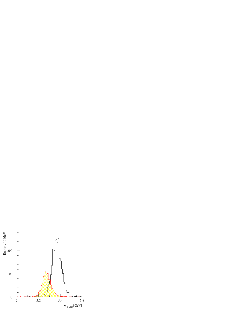
Figure 1: Reconstructed  invariant-mass distribution for $\Bs\to D_{s}^{-}\pi^{+}$ decays. Open histogram: signal, hatched: background from $\bar{B}_{d}^{0}\to D_{s}^{-}\pi^{+}$ decays, dark: fake reconstructed decays from the signal sample. Combinatorial background not shown here.

3 Extraction of significance limits and accuracy for the measurement of $\Delta m_{s}$

3.1 Proper-time reconstruction and resolution

The proper time of the reconstructed   candidates was computed from the reconstructed transverse decay length, $d_{xy}$, and from the  transverse momentum, $p_{\mathrm{T}}$:

$$t=\frac{d_{xy}M_{\Bs}}{cp_{\mathrm{T}}}\equiv d_{xy}g$$

where $g=M_{\Bs}/(cp_{\mathrm{T}})$ and $M_{\Bs}$ is the  mass. Its resolution function $\mathrm{Res}(t\,|\,t_{0})$ was parameterized with the sum of two Gaussian functions, see Eq. (1), with parameters given in Table 2 for the signal channels. Here $t_{0}$ denotes the true (generated) proper time; $f_{\alpha}$ is the fraction and $\sigma_{\alpha}$ the width of the Gaussian function $\alpha$. Similar parameterizations were obtained for the background channels $B_{d}^{0}\to D_{s}^{+}\pi^{-}$ and $B_{d}^{0}\to D_{s}^{+}a_{1}^{-}$.

$$\mathrm{Res}(t\,|\,t_{0})\!\!\! = \!\!f_{1}\frac{1}{\sigma_{1}\sqrt{2\pi}}\;\,\exp\left(-\frac{(t-t_{0})^{2}}{2\,\sigma_{1}^{\;2}}\right)+$$ (1)

$$\!\!f_{2}\frac{1}{\sigma_{2}\sqrt{2\pi}}\;\,\exp\left(-\frac{(t-t_{0})^{2}}{2\,\sigma_{2}^{\;2}}\right)$$

	$\Bs\to D_{s}^{-}\,\pi^{+}$		$\Bs\to D_{s}^{-}\,a_{1}^{+}$
$\alpha$	$f_{\alpha}$ (%)	$\sigma_{\alpha}$(fs)	$f_{\alpha}$ (%)	$\sigma_{\alpha}$(fs)
1	$59.6\pm 6.6$	$\phantom{1}51.5\pm 4.0$	$62.5\pm 14.1$	$\phantom{1}51.6\pm\phantom{1}6.4$
2	$40.4\pm 6.6$	$107.3\pm 8.5$	$37.5\pm 14.1$	$\phantom{1}92.8\pm 12.7$

Table 2: Proper-time resolution function $\mathrm{Res}(t\,|\,t_{0})$ parameterization with the sum of two Gaussian functions.

3.2 Likelihood function

The probability density to observe an initial $B_{j}^{0}$ meson ($j=d,\;s$) decaying at time $t_{0}$ after its creation as a $\bar{B_{j}^{0}}$ meson is given by:

$$p_{j}(t_{0},\;\mu_{0})\!\!\! = \!\!\displaystyle\frac{\Gamma_{j}^{2}-\left(\frac{\Delta\Gamma_{j}}{2}\right)^{2}}{2\,\Gamma_{j}}\>\mathrm{e}^{-\Gamma_{j}t_{0}}\;\times$$ (2)

$$\!\!\left(\cosh\frac{\Delta\Gamma_{j}t_{0}}{2}+\mu_{0}\cos\Delta m_{j}t_{0}\right)$$

where $\Delta\Gamma_{j}=\Gamma_{\mathrm{H}}^{j}-\Gamma_{\mathrm{L}}^{j}$, $\Gamma_{j}=(\Gamma_{\mathrm{H}}^{j}+\Gamma_{\mathrm{L}}^{j})/2$ and $\mu_{0}=-1$. For the unmixed case (an initial $B_{j}^{0}$ meson decays as a $B_{j}^{0}$ meson at time $t_{0}$), the probability density is given by the above expression with $\mu_{0}=+1$.

The above probability is modified by experimental effects: finite proper-time resolution, wrong tags at production or decay, and background. Convolving $p_{j}(t_{0},\;\mu_{0})$ with the proper time resolution $\mathrm{Res}_{j}(t\,|\,t_{0})$, one obtains the probability as a function of $\mu_{0}$ and the reconstructed proper time $t$: $q_{j}(t,\mu_{0})=N\int_{t_{\mathrm{min}}}^{\infty}p_{j}(t_{0},\mu_{0})\;\mathrm{Res}_{j}(t\;|\;t_{0})\;\mathrm{d}t_{0}$, with $N$ a normalization factor and $t_{\mathrm{min}}=0.4$ ps the cut on the  proper decay time. Assuming a fraction $\omega_{j}$ of wrong tags at production or decay, the probability becomes $q_{j}^{\prime}(t,\mu)=(1-\omega_{j})q_{j}(t,\mu)+\omega_{j}q_{j}(t,-\mu)$. Including the background, composed of oscillating $B_{d}^{0}$ mesons and of combinatorial background, with fractions $f_{j}^{k}$ ($j=$ $s$, $d$, and combinatorial background $cb$), one obtains: $\mathrm{pdf}_{k}(t,\mu)=\sum_{j=s,d,cb}f_{j}^{k}\left[(1-\omega_{j})q_{j}(t,\mu)+\omega_{j}q_{j}(t,-\mu)\right]$ where the index $k=1$ denotes the $\Bs\to D_{s}^{-}\pi^{+}$ channel and $k=2$ the $\Bs\to D_{s}^{-}a_{1}^{+}$ channel. The likelihood of the total sample is written as

$${\cal L}(\Delta m_{s},\Delta\Gamma_{s})=\prod_{k=1}^{N_{\mathrm{ch}}}\;\prod_{i=1}^{N_{\mathrm{ev}}^{k}}\mathrm{pdf}_{k}(t_{i},\mu_{i})$$ (3)

where $N_{\mathrm{ev}}^{k}$ is the total number of events of type $k$, and $N_{\mathrm{ch}}=2$.

3.3 Significance limits for the measurement of $\Delta m_{s}$

The ATLAS sensitivity for the $\Delta m_{s}$ measurement was determined using a simplified Monte-Carlo model to produce event samples, combined with the amplitude-fit method [6] to extract the limits. In the amplitude-fit method a new parameter, the  oscillation amplitude ${\cal A}$, is introduced in the likelihood function by replacing the term ‘$\mu_{0}\cos\Delta m_{s}t_{0}$’ with ‘$\mu_{0}{\cal A}\cos\Delta m_{s}t_{0}$’ in the  probability density function. For each value of $\Delta m_{s}$, the new likelihood function is minimized with respect to ${\cal A}$, keeping all other parameters fixed, and a value ${\cal A}\pm\sigma_{\cal A}^{\mathrm{stat}}$ is obtained. The statistical significance $S$ of an oscillation signal can be expressed as $S\approx 1/\sigma_{\cal A}$. One defines a $5\sigma$ significance limit as the value of $\Delta m_{s}$ for which $1/\sigma_{\cal A}=5$, and a sensitivity at 95% confidence limit as the value of $\Delta m_{s}$ for which $1/\sigma_{\cal A}=1.645$.

For $\Delta m_{s}$ values smaller than the $5\sigma$ significance limit, the expected accuracy is estimated using the log-likelihood method, with the likelihood function given by Eq. (3).

3.4 Systematic uncertainties

An attempt to estimate the systematic uncertainties was done. The following contributions to the systematic uncertainties were considered: a relative error of 5% on the wrong-tag fraction for both  and $B_{d}^{0}$; $\pm 1\sigma$ variation of Gaussian-function widths from $\mathrm{Res}(t\,|\,t_{0})$ parameterization; $f_{\Bs}=BR(\bar{b}\to\Bs)$,  lifetime, $\Delta m_{d}$ varied separately by PDG uncertainty; 5% uncertainty for decay time $\tau_{\mathrm{cb}}$ of combinatorial background, keeping the shape exponential. An additional set of ‘projected systematic uncertainties’ was defined, reducing the $f_{\Bs}$ error and the uncertainties on the widths from the proper time parameterization to values expected at the time of ATLAS data taking.

4 Results and conclusions

Table 3 shows the dependence of the amplitude and its statistical and systematic uncertainties on $\Delta m_{s}$ for an integrated luminosity of 10 ${\mathrm{fb}}^{-1}$, for both actual and projected systematic uncertainties. In the generated event samples, the value of $\Delta m_{s}$ was set to $\Delta m_{s}^{\mathrm{gen}}=\infty$, therefore one expects $\sigma_{\cal A}$ compatible with zero. The dominant contributions to the systematic uncertainty come from the uncertainty on the $f_{\Bs}$ fraction and from the parameterization of the proper time resolution.

$\Delta m_{s}$	0 ${\mathrm{ps}}^{-1}$	10 ${\mathrm{ps}}^{-1}$	20 ${\mathrm{ps}}^{-1}$	30 ${\mathrm{ps}}^{-1}$
${\cal A}$	$0.045$	$0.189$	$0.042$	$-0.291$
$\sigma_{\cal A}^{\mathrm{stat}}$	$\pm 0.048$	$\pm 0.090$	$\pm 0.167$	$\pm 0.357$
$\sigma_{\cal A}^{\mathrm{syst}}$	${}^{+0.097\rule[3.01389pt]{0.0pt}{1.50694pt}}_{-0.084\rule[-1.50694pt]{0.0pt}{1.50694pt}}$	${}^{+0.130}_{-0.096}$	${}^{+0.180}_{-0.142}$	${}^{+0.298}_{-0.226}$
with ‘projected systematic uncertainties’
$\sigma_{\cal A}^{\mathrm{syst}}$	${}^{+0.049\rule[3.01389pt]{0.0pt}{1.50694pt}}_{-0.049\rule[-1.50694pt]{0.0pt}{1.50694pt}}$	${}^{+0.060}_{-0.048}$	${}^{+0.085}_{-0.066}$	${}^{+0.137}_{-0.117}$

Table 3: The oscillation amplitude ${\cal A}$ and its statistical and systematic uncertainties as a function of $\Delta m_{s}$ for an integrated luminosity of 10 ${\mathrm{fb}}^{-1}$.

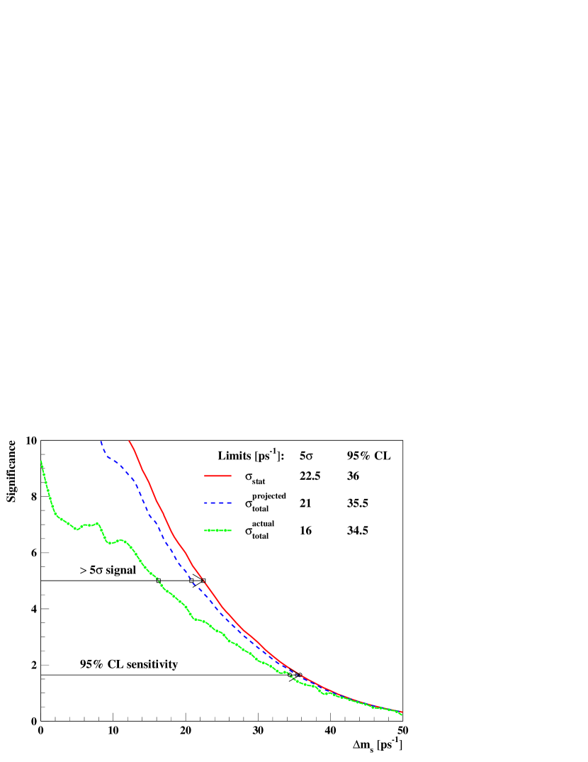
Figure 2: The significance of the  oscillation signal as a function of $\Delta m_{s}$ for an integrated luminosity of 10 ${\mathrm{fb}}^{-1}$.

The significance of the  oscillation signal as a function of $\Delta m_{s}$ for an integrated luminosity of 10 ${\mathrm{fb}}^{-1}$is shown in Fig. 2. The $5\sigma$ significance limit is 22.5 ${\mathrm{ps}}^{-1}$ and the 95% CL sensitivity is 36.0 ${\mathrm{ps}}^{-1}$, when computed with the statistical uncertainty only. Computed with the total uncertainty, the $5\sigma$ significance limit is 16.0 ${\mathrm{ps}}^{-1}$ and the 95% CL sensitivity is 34.5 ${\mathrm{ps}}^{-1}$ for the actual systematic uncertainties, and 21 ${\mathrm{ps}}^{-1}$ and 35.5 ${\mathrm{ps}}^{-1}$ for the projected systematic uncertainties. The limits for other values of the integrated luminosity are given in Table 4, computed with the statistical uncertainties only.

Luminosity	$5\sigma$ limit	$95\%$ CL sensitivity
(${\mathrm{fb}}^{-1}$)	(${\mathrm{ps}}^{-1}$)	(${\mathrm{ps}}^{-1}$)
15	17.5	32.0
10	22.5	36.0
20	27.0	39.0
30	29.5	41.0

Table 4: The dependence of significance limits for the $\Delta m_{s}$ measurement on the integrated luminosity, computed with statistical uncertainties only.

The dependence of the significance limits on $\Delta\Gamma_{s}/\Gamma_{s}$  was also estimated. For values of $\Delta\Gamma_{s}/\Gamma_{s}$ up to 30%, no sizeable effect was observed. The shape and the fraction of the combinatorial background were also varied within reasonable values; only a weak dependence of the limits was observed.

For $\Delta m_{s}$ values smaller than the $5\sigma$ significance limit, the accuracy of the $\Delta m_{s}$ measurement was determined for different values of the integrated luminosity. The results are given in Table 5. If measured, the precision on $\Delta m_{s}$ will be dominated by the statistical errors.

Luminosity	$\Delta m_{s}^{\mathrm{gen}}$	$\Delta m_{s}^{\mathrm{rec}}\pm\sigma^{\Delta m_{s}}_{\mathrm{stat}}\pm\sigma^{\Delta m_{s}}_{\mathrm{syst}}$	Obs.
(${\mathrm{fb}}^{-1}$)	(${\mathrm{ps}}^{-1}$)	(${\mathrm{ps}}^{-1}$)
1 5	$17.5$	$17.689\pm 0.083\pm 0.002$	$5\sigma$ lim.
	$15.0$	$15.021\pm 0.049\pm 0.002$
10	$22.5$	$22.396\pm 0.072\pm 0.005$	$5\sigma$ lim.
	$15.0$	$14.949\pm 0.033\pm 0.002$
20	$20.0$	$20.041\pm 0.068\pm 0.005$
	$27.0$	$26.948\pm 0.070\pm 0.003$	$5\sigma$ lim.
	$15.0$	$14.942\pm 0.028\pm 0.004$
30	$20.0$	$20.010\pm 0.043\pm 0.002$
	$29.5$	$29.708\pm 0.083\pm 0.007$	$5\sigma$ lim.

Table 5: The accuracy of $\Delta m_{s}$ measurement as a function of the integrated luminosity. $\sigma^{\Delta m_{s}}_{\mathrm{stat}}$ represents the statistical uncertainty, $\sigma^{\Delta m_{s}}_{\mathrm{stat}}$ the systematic uncertainty. The $5\sigma$ limits were computed with statistical errors only.

5 Recent developments

This section summarizes recent changes of the assumptions or conditions used to get the results presented above.

The most important changes in the detector geometry are the increase of the beam-pipe diameter from 41.5 mm to 50.5 mm and the increase of the pixel length in B-layer, the closest layer to the beam-pipe, from 300 ${\mu}$m to 400 ${\mu}$m.

Due to financial constraints, the B-physics trigger resources have to be minimized. Previously, dedicated resources were supposed to be available for the B-physics trigger, in addition to resources for high-$p_{\mathrm{T}}$ physics trigger (‘discovery physics trigger’). It may not be possible to provide any significant additional resources. Moreover, there are financial uncertainties which could lead to the deferral of some detector items, therefore it is possible to have a reduced detector at start-up. Items included in the deferral scenario are the second pixel layer from the Inner Detector, resulting in a two-layer pixel detector, the $\eta>2$ region of the Transition Radiation Detector from the Inner Detector, and a significant part of the processors for level-2 and event filter, reducing the computing resources for the high-level trigger and limiting the level-1 rate.

The luminosity target for LHC start-up doubled to $2\times 10^{33}$ cm^-2s^-1, therefore it will be necessary to re-evaluate trigger thresholds and to remove some triggers requiring too much resources. The trigger for  oscillation channels requires a significant rate, therefore it is very likely that the muon trigger threshold will be raised to $\sim 8$ GeV.

Recent work concentrates on trigger-related issues; improvements of the offline analysis, although possible, have to be postponed. To reduce the resource requirements, one of the possibilities would be to change the trigger for $B$ hadronic channels from $\mu(p_{\mathrm{T}}>6\;\mathrm{GeV})$ at level-1 plus Inner Detector full scan at Level-2 to $\mu(p_{\mathrm{T}}>6\;\mathrm{GeV})$ at level-1, plus a low $E_{T}$ level-1 calorimeter Region-of-Interest (RoI), used then to guide reconstruction at level-2. In addition, one can use the level-2 RoI to limit the region for reconstruction at the event filter. A flexible trigger and analysis strategy is nowadays evaluated, which should be able to cope with detector changes, luminosity scenarios, financial problems. Another direction is to recover performance using optimized reconstruction algorithms, flexible trigger and analysis thresholds. A re-evaluation of the detector performance with the latest geometry is also under way. Preliminary results are encouraging.

References

-
[1]
The LEP Working group on B oscillations,
Combined results for Winter 2003 conferences, http://lepbosc.web.cern.ch/LEPBOSC/ - [2] M.Battaglia, A. Buras, P. Gambino and A. Stocchi, eds. The CKM Matrix and the Unitarity Triangle (hep-ph/0304132), to be published as CERN Yellow Book.
- [3] B. Epp, V.M. Ghete and A. Nairz, EPJdirect CN3 (2002) 1.
- [4] T. Sjöstrand, Comp. Phys. Comm. 82 (1994) 74.
- [5] Particle Data Group: C. Caso et al., Review of Particle Physics, Euro. Phys. J. C3 (1998) 1.
- [6] H.G. Moser and A. Roussarie, Nucl. Instr. Meth. A384 (1997) 491.