Hard Loops, Soft Loops, and High Density Effective Field Theory

Abstract

We study several issues related to the use of effective field theories in QCD at large baryon density. We show that the power counting is complicated by the appearance of two scales inside loop integrals. Hard dense loops involve the large scale $\mu^{2}$ and lead to phenomena such as screening and damping at the scale $g\mu$. Soft loops only involve small scales and lead to superfluidity and non-Fermi liquid behavior at exponentially small scales. Four-fermion operators in the effective theory are suppressed by powers of $1/\mu$, but they get enhanced by hard loops. As a consequence their contribution to the pairing gap is only suppressed by powers of the coupling constant, and not powers of $1/\mu$. We determine the coefficients of four-fermion operators in the effective theory by matching quark-quark scattering amplitudes. Finally, we introduce a perturbative scheme for computing corrections to the gap parameter in the superfluid phase.

I Introduction

The study of baryonic matter in the regime of high baryon density has led to the discovery of new phases of strongly interacting matter, such as color superconducting quark matter and color-flavor locked matter Bailin:1984bm ; Alford:1998zt ; Rapp:1998zu ; Alford:1999mk ; Rajagopal:2000wf ; Alford:2001dt ; Schafer:2003vz ; Rischke:2003mt . These phases are not only relevant to the structure of compact astrophysical objects Reddy:2002ri ; Alford:wf , but they also provide a theoretical laboratory in which complicated QCD phenomena, such as chiral symmetry breaking and the formation of a mass gap, can be studied in a weakly coupled setting Schafer:1999ef . In order to exploit these opportunities we would like to develop a systematic framework that will allow us to determine the exact nature of the phase diagram as a function of the density, temperature, the quark masses, and the lepton chemical potentials, and to compute the low energy properties of these phases.

If the density is large then the Fermi momentum is much bigger than the QCD scale, $p_{F}=\mu\gg\Lambda_{QCD}$, and it would seem that such a framework is provided by perturbative QCD. It is clear, however, that a naive expansion in powers of $\alpha_{s}$ is not sufficient. First of all, it is well known that resummation is required in order to make the perturbative expansion in a many body system well defined GellMann:1957 . It is also well known that additional problems arise in systems with unscreened transverse gauge boson interactions Holstein:1973 ; Reizer:1989 . In a degenerate Fermi system the effect of the BCS or other pairing instabilities have to be taken into account. And finally, in systems with broken global symmetries, the low energy properties of the system are governed by collective modes that carry the quantum numbers of the broken generators.

In order to address these problems it is natural to exploit the separation of scales provided by $\mu\gg g\mu\gg\Lambda_{QCD}$ in the normal phase, or $\mu\gg g\mu\gg\Delta\gg\Lambda_{QCD}$ in the superfluid phase. An effective field theory approach to phenomena near the Fermi surface was suggested by Hong Hong:2000tn ; Hong:2000ru . This approach was applied to the gap equation Beane:2000ji , Goldstone boson masses Beane:2000ms ; Schafer:2001za , gluon dispersion relations Casalbuoni:2001ha , and a number of other problems. For a review and further references, see Nardulli:2002ma . Even though a number of interesting results have been obtained there are a number of important conceptual issues that are not very well understood. These issues concern power counting, renormalization and matching. In this work we would like to study some of these issues in more detail. This paper is organized as follows. In section II we give a review of the standard hard thermal loop approximation applied to dense matter. In Section III we introduce the high density and effective theory (HDET) and in Section IV we show how hard dense loops (HDLs) arise in the effective theory. In Section V we show that the effective theory contains a new class of diagrams which we shall call soft dense loops. In Sections VI and VII we study the gap equation at leading and next-to-leading order and in Section VIII we study matching conditions for four-fermion operators.

II Hard Dense Loops

In this section we review the calculation of hard dense loop contributions to QCD Greens functions Braaten:1989mz ; Blaizot:1993bb ; Manuel:1995td . The hard dense loop limit corresponds to soft external momenta, $|\vec{p}|\ll\mu$. In this limit the main medium contribution comes from hard loop momenta, $|\vec{k}|\sim\mu$. Our main purpose in this section is to present a simple rederivation of the main results that will allow us to compare the hard dense loop approximation with the high density effective theory which is discussed in section III.

Hard dense loops can be calculated most simply by writing the free fermion propagator at $\mu\neq 0$ in the form

$$S(k)=\frac{1}{2}\left\{\frac{\hat{K}\!\!\!\!/\,}{k_{0}-\epsilon^{+}_{k}}+\frac{\hat{\bar{K}}\!\!\!\!/\,}{k_{0}-\epsilon^{-}_{k}}\right\},$$ (1)

where $\epsilon_{k}^{\pm}=\pm(|\vec{k}|\mp\mu)$ and $\hat{K}=(1,\hat{k})$, $\hat{\bar{K}}=(1,-\hat{k})$ with $\hat{k}=\vec{k}/|\vec{k}|$. The two poles of the propagator in equ. (1) correspond to particle and anti-particle states. Note that $\Lambda_{k}^{+}=\hat{K}\!\!\!\!/\,\gamma_{0}/2$ and $\Lambda_{k}^{-}=\hat{\bar{K}}\!\!\!\!/\,\gamma_{0}/2$ are projection operators on positive and negative energy solutions of the free Dirac equation. Also observe that $(\hat{K}\!\!\!\!/\,)^{2}=(\hat{\bar{K}}\!\!\!\!/\,)^{2}=0$ which is very useful in evaluating Dirac traces in the hard dense loop approximation. In our convention the energy is measured relative to the Fermi energy $\mu$. In order to derive HDL Greens functions it is useful to define the energy of a fermion as $\omega=k_{0}+\mu$. The HDL limit corresponds to $\omega,|\vec{k}|\ll\mu$, whereas quasi-particles in the vicinity of the Fermi surface satisfy $\omega,|\vec{k}|\sim\mu$.

As an example, let us consider the calculation of the gluon polarization function. The one-loop contribution is given by

$$\Pi_{\mu\nu}^{ab}(p)=N_{f}g^{2}\frac{\delta^{ab}}{2}\int\frac{d^{4}k}{(2\pi)^{4}}{\rm Tr}\left(\gamma_{\mu}S(k)\gamma_{\nu}S(k-p)\right).$$ (2)

If the propagator is written in terms of particle and anti-particle contributions as in equ. (31) we find three contributions to the polarization function, the particle-hole, particle-anti-particle, and anti-particle-anti-hole terms. The particle-hole contribution shown in Fig.1a is

$$\left.\Pi_{\mu\nu}^{ab}(p)\right|_{ph}=2m^{2}\delta^{ab}\int\frac{d\Omega}{4\pi}\hat{K}_{\mu}\hat{K}_{\nu}\left\{1-\frac{p_{0}}{p\cdot\hat{K}}\right\}$$ (3)

where $m^{2}=N_{f}g^{2}\mu^{2}/(4\pi^{2})$. This contribution is dominated by loop momenta $|\vec{k}|\sim\mu$ very close to the Fermi surface. However, the particle-hole term is not transverse Hong:2000ru ; Rischke:2000qz . The particle-anti-particle term is

$$\left.\Pi_{\mu\nu}^{ab}(p)\right|_{pa}=2m^{2}\delta^{ab}\int\frac{d\Omega}{4\pi}\left\{\delta_{\mu 0}\delta_{\nu 0}-\hat{K}_{\mu}\hat{K}_{\nu}\right\}.$$ (4)

Note that this term receives contributions from particles with momenta in the range $0\leq|\vec{k}|\leq\mu$, and not only particles in the vicinity of the Fermi surface. Also note that in the hard dense loop limit this term is just a constant, with no momentum dependence. The sum of the two contributions equ. (3) and (4) is given by

$$\Pi_{\mu\nu}^{ab}(p)=2m^{2}\delta^{ab}\int\frac{d\Omega}{4\pi}\left\{\delta_{\mu 0}\delta_{\nu 0}-\frac{p_{0}\hat{K}_{\mu}\hat{K}_{\nu}}{p\cdot\hat{K}}\right\}.$$ (5)

The polarization tensor equ. 5) is transverse and agrees with the well known hard dense loop result.

The fermion self energy in the hard dense loop approximation is given by Blaizot:1993bb

$$\Sigma(p)=m_{f}^{2}\int\frac{d\Omega}{4\pi}\frac{\hat{K}\!\!\!\!/\,}{p\cdot\hat{K}},$$ (6)

with $m_{f}^{2}=C_{F}g^{2}\mu^{2}/(8\pi^{2})$ and $C_{F}=(N_{c}^{2}-1)/(2N_{c})$. This result arises solely from the particle term in the fermion propagator equ. (31). The loop integral receives contributions from all momenta $0\leq|\vec{k}|\leq\mu$. It is important to emphasize that the HDL approximation corresponds to external momenta that are soft, $|\vec{p}|\ll\mu$, whereas low energy fermionic excitations have momenta $|\vec{p}|\sim\mu$. The use of the HDL fermion self energy is not reliable for low energy modes. It is nevertheless instructive to study the behavior of the HDL self energy near the Fermi surface. Using equ. (6) we find

$$\Sigma(p)=\Sigma_{S}(p)-\Sigma_{V}(p)\vec{\gamma}\cdot\hat{p}$$ (7)

with

$$\Sigma_{S}(p) = \frac{m_{f}^{2}}{|\vec{p}|}Q_{0}\left(\frac{\omega}{|\vec{p}|}\right),\hskip 42.67912ptQ_{0}\left(\frac{\omega}{|\vec{p}|}\right)=\frac{1}{2}\log\left(\frac{\omega+|\vec{p}|}{\omega-|\vec{p}|}\right),$$ (8)

$$\Sigma_{S}(p) = -\frac{m_{f}^{2}}{|\vec{p}|}\left(1-\frac{\omega}{|\vec{p}|}Q_{0}\left(\frac{\omega}{|\vec{p}|}\right)\right).$$ (9)

We observe that both $\Sigma_{S}$ and $\Sigma_{V}$ are logarithmically divergent near the Fermi surface, but the quasi-particle dispersion relation and the wave function renormalization factor are well behaved. Indeed, for the particle mode

$$S(p)=(S_{0}^{-1}(p)-\Sigma(p))^{-1}\simeq\frac{Z_{+}(p)}{p_{0}-\omega^{+}_{p}}\frac{\hat{P}\!\!\!\!/\,}{2}+\ldots,$$ (10)

with

$$\omega_{+}(p)\simeq|\vec{p}|+\frac{m_{f}^{2}}{|\vec{p}|},\hskip 14.22636ptZ_{+}(p)\simeq 1+\frac{m_{f}^{2}}{2|\vec{p}|^{2}}\left(1-\log\left(\frac{2|\vec{p}|^{2}}{m_{f}^{2}}\right)\right).$$ (11)

At one-loop order the quark-gluon vertex receives contributions from the abelian diagram Fig. 3a and the non-abelian diagram Fig. 3b. In the HDL limit these two diagrams are identical up to a color factor. We find

$$\Gamma_{\mu}(p_{1},p_{2})=-m_{f}^{2}\int\frac{d\Omega}{4\pi}\frac{\hat{K}_{\mu}\hat{K}\!\!\!\!/\,}{(p_{1}\cdot\hat{K})(p_{2}\cdot\hat{K})},$$ (12)

where $p_{1},p_{2}$ are the momenta of the two fermions and we have factored out the color structure $\lambda^{a}/2$. The vertex correction is similar to the fermion self energy in the sense that the loop integral receives contribution from momenta $0\leq|\vec{k}|\leq\mu$. Also, we can study the effect of the HDL effective vertex for quasi-particles in the vicinity of the Fermi surface. Since both the incoming and outgoing Fermions are hard the interesting regime corresponds to soft gluon momenta. In this limit the matrix element of the free vertex between projectors on quasi-particle states with momentum $p$ is $\langle\gamma_{\mu}\rangle=\hat{P}_{\mu}$. For the HDL vertex correction we find

$$\langle\Gamma_{\mu}(p,p^{\prime})\rangle=-\frac{m_{f}^{2}}{\mu}\int\frac{d\Omega}{4\pi}\frac{\hat{K}_{\mu}}{p^{\prime}\cdot\hat{K}},$$ (13)

which has a logarithmic divergence near the Fermi surface.

The gluonic three-point function in the HDL limit only receives contributions from the fermion loop diagram shown in Fig. 2a. We find

$$\Gamma^{abc}_{\mu\nu\alpha}(p,q,r)=igf^{abc}2m^{2}\int\frac{d\Omega}{4\pi}\hat{K}_{\mu}\hat{K}_{\alpha}\hat{K}_{\beta}\left\{\frac{q_{0}}{(q\cdot\hat{K})(p\cdot\hat{K})}-\frac{r_{0}}{(r\cdot\hat{K})(p\cdot\hat{K})}\right\}.$$ (14)

The three-point function, as well as higher $n$-point functions, is dominated by momenta near the Fermi surface. Also, as opposed to the case of the two-point function, anti-particles only make sub-leading contributions. Higher $n$-point functions can be computed directly using the methods discussed here. Alternatively, as is the case for $T\neq 0$, $n\geq 3$ point functions can be reconstructed using Ward identities or non-local effective actions. To summarize this section, we showed that gluon $n$-point functions in the HDL limit are dominated by modes near the Fermi surface. The only exception is the two-point function which requires a contact term determined by modes with momenta between zero and the Fermi momentum. Fermion HDLs, on the other hand, are always determined by momenta in the range $0\leq|\vec{k}|\leq\mu$. We emphasized, however, that the HDL limit is not relevant for low energy fermionic excitations.

III High Density Effective Theory (HDET)

In this work we wish to compare the hard dense loop results with the Greens functions obtained from an effective theory which describes low energy excitations in the vicinity of the Fermi surface. The leading order terms in the effective theory are Hong:2000tn ; Hong:2000ru ; Beane:2000ms

$${\cal L}=\sum_{v}\psi_{v}^{\dagger}(iv\cdot D)\psi_{v}-\frac{1}{4}G^{a}_{\mu\nu}G^{a}_{\mu\nu}+\ldots,$$ (15)

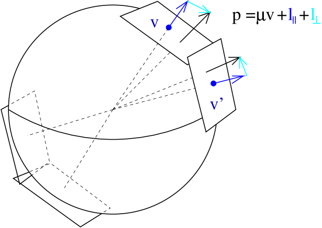
Figure 4: High density effective field theory description of excitations near the Fermi surface. The effective theory is defined on patches labeled by the local Fermi velocity $v$. Momenta are decomposed with respect to $v$, $\vec{p}=\mu\vec{v}+l_{\perp}+l_{||}$.

where $v_{\mu}=(1,\vec{v})$. In the vicinity of the Fermi surface the relevant degrees of freedom are particle and hole excitations which move with the Fermi velocity $v$. We shall describe these excitations in terms of a field $\psi_{v}(x)$. This field describes particles and holes with momenta $p=\mu\vec{v}+l$, where $l\ll\mu$. We will write $l=l_{0}+l_{\|}+l_{\perp}$ with $\vec{l}_{\|}=\vec{v}(\vec{l}\cdot\vec{v})$ and $\vec{l}_{\perp}=\vec{l}-\vec{l}_{\|}$. In order to take into account the entire Fermi surface we have to cover the Fermi surface with patches labeled by the local Fermi velocity, see Fig. 4. The number of such patches is $n_{v}\sim(\mu^{2}/\Lambda_{\perp}^{2})$ where $\Lambda_{\perp}\ll\mu$ is the cutoff on the transverse momenta $l_{\perp}$.

Higher order terms are suppressed by powers of $1/\mu$. As usual we have to consider all possible terms allowed by the symmetries of the underlying theory. At $O(1/\mu)$ we have

$${\cal L}=\sum_{v}\left\{-\frac{1}{2\mu}\psi_{v}^{\dagger}D_{\perp}^{2}\psi_{v}-ag\psi_{v}^{\dagger}\frac{\sigma^{\mu\nu}G_{\mu\nu}^{\perp}}{4\mu}\psi_{v}\right\}.$$ (16)

The coefficient of the first term is fixed by the dispersion relation of a fermion near the Fermi surface, $l_{0}=l_{\|}+l_{\perp}^{2}/(2\mu)+\ldots$. The coefficient of the second term is most easily determined by writing the quark field in the microscopic theory as $\psi=\psi_{+}+\psi_{-}$ and then integrating out $\psi_{-}$ at tree level. We find $a=1+O(g^{2})$, where the $O(g^{2})$ terms arise from higher order perturbative corrections. At higher order in $1/\mu$ there is an infinite tower of operators of the form $\mu^{-n}\psi^{\dagger}_{v}D_{\perp}^{2n_{1}}(\bar{v}\cdot D)^{n_{2}}\psi_{v}$ with $\bar{v}=(1,-\vec{v})$ and $n=2n_{1}+n_{2}-1$.

At $O(1/\mu^{2})$ the effective theory contains four-fermion operators

$${\cal L}=\frac{1}{\mu^{2}}\sum_{v_{i}}\sum_{\Gamma,\Gamma^{\prime}}c^{\Gamma\Gamma^{\prime}}(\vec{v}_{1}\cdot\vec{v}_{2},\vec{v}_{1}\cdot\vec{v}_{3},\vec{v}_{2}\cdot\vec{v}_{3})\Big{(}\psi_{v_{1}}\Gamma\psi_{v_{2}}\Big{)}\Big{(}\psi^{\dagger}_{v_{3}}\Gamma^{\prime}\psi^{\dagger}_{v_{4}}\Big{)}\delta_{v_{1}+v_{2}-v_{3}-v_{4}}.$$ (17)

The restriction $v_{1}+v_{2}=v_{3}+v_{4}$ allows two types of four-fermion operators. The first possibility is that both the incoming and outgoing fermion momenta are back-to-back. This corresponds to the BCS interaction

$${\cal L}=\frac{1}{\mu^{2}}\sum_{v,v^{\prime}}\sum_{\Gamma,\Gamma^{\prime}}V_{l}^{\Gamma\Gamma^{\prime}}R_{l}^{\Gamma\Gamma^{\prime}}(\vec{v}\cdot\vec{v}^{\prime})\Big{(}\psi_{v}\Gamma\psi_{-v}\Big{)}\Big{(}\psi^{\dagger}_{v^{\prime}}\Gamma^{\prime}\psi^{\dagger}_{-v^{\prime}}\Big{)},$$ (18)

where $\vec{v}\cdot\vec{v}^{\prime}=\cos\theta$ is the scattering angle and $R_{l}^{\Gamma\Gamma^{\prime}}(\vec{v}\cdot\vec{v}^{\prime})$ is a set of orthogonal polynomials that we will specify below. The second possibility is that the final momenta are equal to the initial momenta up to a rotation around the axis defined by the sum of the incoming momenta. The relevant four-fermion operator is

$${\cal L}=\frac{1}{\mu^{2}}\sum_{v,v^{\prime},\phi}\sum_{\Gamma,\Gamma^{\prime}}F_{l}^{\Gamma\Gamma^{\prime}}(\phi)R_{l}^{\Gamma\Gamma^{\prime}}(\vec{v}\cdot\vec{v}^{\prime})\Big{(}\psi_{v}\Gamma\psi_{v^{\prime}}\Big{)}\Big{(}\psi^{\dagger}_{\tilde{v}}\Gamma^{\prime}\psi^{\dagger}_{\tilde{v}^{\prime}}\Big{)},$$ (19)

where $\tilde{v},\tilde{v}^{\prime}$ are the vectors obtained from $v,v^{\prime}$ by a rotation around $v_{tot}=v+v^{\prime}$ by the angle $\phi$. In a system with short range interactions only the quantities $F_{l}(0)$ are known as Fermi liquid parameters. The matrices $\Gamma,\Gamma^{\prime}$ describe the spin, color and flavor structure of the interaction. In the following we will focus on the spin structure. We can decompose

$$\Big{(}\Gamma\Big{)}\Big{(}\Gamma^{\prime}\Big{)}=\left\{\Big{(}H_{\pm}^{T}\sigma_{2}H_{\pm}\Big{)}\Big{(}H_{\pm}^{T}\sigma_{2}H_{\pm}\Big{)},\Big{(}H_{\pm}^{T}\sigma_{2}\vec{\sigma}H_{\pm}\Big{)}\Big{(}H_{\pm}^{T}\sigma_{2}\vec{\sigma}H_{\pm}\Big{)}\right\},$$ (20)

where $H_{\pm}=(1\pm\vec{v}\cdot\vec{\sigma})/2$ are helicity projectors. In the spin zero sector there are two possible helicity channels, $(++)\to(++)$ and $(++)\to(--)$ together with their parity partners $(+\leftrightarrow-)$. In the limit $m\to 0$ perturbative interactions only contribute to the helicity non-flip amplitude

$${\cal L}=\frac{1}{\mu^{2}}\sum_{v,v^{\prime}}V_{l}^{++}P_{l}(\vec{v}\cdot\vec{v}^{\prime})\Big{(}\psi_{v}\sigma_{2}H_{+}\psi_{-v}\Big{)}\Big{(}\psi^{\dagger}_{v^{\prime}}\sigma_{2}H_{+}\psi^{\dagger}_{-v^{\prime}}\Big{)}+(+\leftrightarrow-),$$ (21)

where $P_{l}(\cos\theta)$ are Legendre polynomials. At $O(m^{2}/\mu^{2})$ quark mass terms induce a non-zero helicity flip amplitude. The corresponding four-fermion operator was determined in Schafer:2001za . In $N_{f}=2$ QCD instantons generate a helicity-flip amplitude which is suppressed by extra powers of $(\Lambda_{QCD}/\mu)$ Schafer:1999na . In QCD with $N_{f}=3$ flavors instantons produce a helicity changing four-fermion interaction which is suppressed by both $(\Lambda_{QCD}/\mu)$ and $(m/\mu)$ Schafer:2002ty . Even though helicity changing amplitudes are suppressed, they have important physical effects. For example, helicity flip amplitudes determine the masses of Goldstone bosons in the CFL and 2SC phase.

In the spin one sector there is only one helicity channel $(+-)\to(+-)$. The corresponding BCS interaction is

$${\cal L}=\frac{1}{\mu^{2}}\sum_{v,v^{\prime}}V_{l}^{+-}d^{(l)}_{11}(\vec{v}\cdot\vec{v}^{\prime})\Big{(}\psi_{v}\sigma_{2}H_{-}\vec{\sigma}H_{+}\psi_{-v}\Big{)}\Big{(}\psi^{\dagger}_{v^{\prime}}\sigma_{2}H_{-}\vec{\sigma}H_{+}\psi^{\dagger}_{-v^{\prime}}\Big{)}+(+\leftrightarrow-),$$ (22)

where $d^{(l)}_{11}(\cos\theta)$ is the reduced Wigner D-function. For details on the helicity amplitude formalism we refer the reader to Jacob:at . Note that in the total helicity zero channel the reduced rotation matrix reduces to a Legendre polynomial, $d^{(l)}_{00}(\cos\theta)=P_{l}(\cos\theta)$, in agreement with equ. (21). We will discuss the matching conditions for the the spin zero and spin one BCS helicity amplitudes $V_{l}^{++}$ and $V_{l}^{+-}$ in Sect. VIII.

IV Hard Loops

There are two types of loop diagrams that arise in high density effective field theory, hard dense loops and soft dense loops. As an example of a hard dense loop we study the gluon two point function. At leading order in $g$ and $1/\mu$ we have

$$\Pi^{ab}_{\mu\nu}(p)=2g^{2}N_{f}\frac{\delta^{ab}}{2}\sum_{\vec{v}}v_{\mu}v_{\nu}\int\frac{d^{4}k}{(2\pi)^{4}}\frac{1}{(k_{0}-l_{k})(k_{0}+p_{0}-l_{k+p})},$$ (23)

where $l_{k}=\vec{v}\cdot\vec{k}$. We note that taking the momentum of the external gluon to zero automatically selects forward scattering. We also observe that the gluon can interact with fermions of any Fermi velocity so that the polarization function involves a sum over all patches. After performing the $k_{0}$ integration we get

$$\Pi^{ab}_{\mu\nu}(p)=2g^{2}N_{f}\frac{\delta^{ab}}{2}\sum_{\vec{v}}v_{\mu}v_{\nu}\int\frac{d^{2}l_{\perp}}{(2\pi)^{2}}\int\frac{dl_{k}}{2\pi}\frac{l_{p}}{p_{0}-l_{p}}\frac{\partial n_{k}}{\partial l_{k}},$$ (24)

where $n_{k}$ is the Fermi distribution function. We note that the $l_{k}$ integration is automatically restricted to small momenta. The integral over the transverse momenta $l_{\perp}$, on the other hand, diverges quadratically with the cutoff $\Lambda_{\perp}$. We observe, however, that the sum over patches and the integral over $l_{\perp}$ can be combined into an integral over the entire Fermi surface

$$\frac{1}{2\pi}\sum_{\vec{v}}\int\frac{d^{2}l_{\perp}}{(2\pi)^{2}}=\frac{\mu^{2}}{2\pi^{2}}\int\frac{d\Omega}{4\pi}.$$ (25)

This identification is consistent with our observation that the number of patches is $n\sim\mu^{2}/(2\pi^{2}\Lambda_{\perp}^{2})$. As a consequence of equ. (25) the upper limit of the $l_{\perp}$ integral is effectively $\mu$, and not $\Lambda_{\perp}\ll\mu$. We will refer to loop integrals of this kind as hard loops. We find

$$\Pi^{ab}_{\mu\nu}(p)=2m^{2}\delta^{ab}\int\frac{d\Omega}{4\pi}v_{\mu}v_{\nu}\left\{1-\frac{p_{0}}{p_{0}-l_{p}}\right\}.$$ (26)

This result agrees with equ. (3). We know however, that equ. (26) is not transverse and that the contribution from anti-particles, equ. (4) is missing. In the effective theory, this contribution has to represented by a local counterterm. The required counterterm is Hong:2000tn

$${\cal L}=\frac{1}{2}m^{2}\int\frac{d\Omega}{4\pi}(\vec{A}_{\perp})^{2}.$$ (27)

The appearance of this term is related to the fact that terms in the lagrangian of the form $\mu^{-n}\psi^{\dagger}_{v}D_{\perp}^{2n_{1}}(\bar{v}\cdot D)^{n_{2}}\psi_{v}$ give non-vanishing tadpole contributions proportional to $g^{2n_{1}+n_{2}}\mu^{4-2n_{1}-n_{2}}A_{\perp}^{2n_{1}}(\bar{v}\cdot A)^{n2}$ which have to be absorbed into counterterms.

Putting everything together we find

$$\Pi_{\mu\nu}(p)=2m^{2}\int\frac{d\Omega}{4\pi}\left\{\delta_{\mu 0}\delta_{\nu 0}-\frac{v_{\mu}v_{\nu}p_{0}}{p_{0}-l_{p}}\right\}$$ (28)

which agrees with the complete HDL result equ. (5). The gluonic three-point function can be computed in the same fashion. Using the rule equ. (25) we find

$$\Gamma^{abc}_{\mu\nu\alpha}(p,q,r)=igf^{abc}2m^{2}\int\frac{d\Omega}{4\pi}v_{\mu}v_{\alpha}v_{\beta}\left\{\frac{q_{0}}{(q\cdot v)(p\cdot v)}-\frac{r_{0}}{(r\cdot v)(p\cdot v)}\right\},$$ (29)

which agrees with the HDL result equ. (14). We note that in the case of the three point function, as well as higher $n$-point functions, there is no leading order contribution from anti-particle states, and this is reflected by the absence of counterterms at leading order in the effective theory.

V Soft Loops

As an example of a soft loop contribution in the high density effective theory we study the fermion self energy. At leading order, we have

$$\Sigma(p)=g^{2}C_{F}\int\frac{d^{4}k}{(2\pi)^{4}}\frac{1}{p_{0}+k_{0}-l_{p+k}}v_{\mu}v_{\nu}D_{\mu\nu}(k),$$ (30)

where $D_{\mu\nu}(k)$ is the gluon propagator. Soft contributions to the quark self energy are dominated by nearly forward scattering. Note that this loop integral does not involve a sum over patches. Hard contributions to the fermion self energy are governed by the four-fermion operators equ. (19). We saw in the previous section that hard loops cause non-perturbative effects in gluon $n$-point functions at the scale $g\mu$. At energies below this scale we have to replace the free gluon term in the effective lagrangian by the generating functional for hard dense loops Braaten:1991gm ; Braaten:1992jj

$${\cal L}=-m^{2}\int\frac{d\Omega}{4\pi}{\rm Tr}\,G_{\mu\alpha}\frac{\hat{P}^{\alpha}\hat{P}^{\beta}}{(\hat{P}\cdot D)^{2}}G^{\mu}_{\,\beta},$$ (31)

where the angular integral corresponds to an average over the direction of $\hat{P}_{\alpha}=(1,\hat{p})$. Note that the effective gluonic action is non-local. The effective fermion action in the high density effective theory for momenta below $g\mu$ remains local. The hard dense loop effective action equ. (31) leads to the gluon propagator

$$D_{\mu\nu}(k)=\frac{P_{\mu\nu}^{T}}{k^{2}-\Pi_{M}}+\frac{P_{\mu\nu}^{L}}{k^{2}-\Pi_{E}}$$ (32)

where $\Pi_{M}$ and $\Pi_{E}$ are the transverse and longitudinal self energies in the HDL limit. The projection operators $P_{\mu\nu}^{T,L}$ are defined by

$$P_{ij}^{T} = \delta_{ij}-\hat{k}_{i}\hat{k}_{j},\hskip 28.45274ptP_{00}^{T}=P_{0i}^{T}=0,$$ (33)

$$P_{\mu\nu}^{L} = -g_{\mu\nu}+\frac{k_{\mu}k_{\nu}}{k^{2}}-P_{\mu\nu}^{T}.$$ (34)

In the regime $|k_{0}|<|\vec{k}|<g\mu$ the self energies can be approximated by $\Pi_{E}=2m^{2}$ and $\Pi_{M}=i\frac{\pi}{2}m^{2}k_{0}/|\vec{k}|$. We note that in this regime the transverse self energy is much smaller than the longitudinal one, $\Pi_{M}<\Pi_{E}$. As a consequence the dominant part of the fermion self energy arises from transverse gluons. We have

$$\Sigma(p)=g^{2}C_{F}\int\frac{dl_{0}}{2\pi}\int\frac{l^{2}dl}{(2\pi)^{2}}\int_{-1}^{1}dx\frac{1-x^{2}}{p_{0}+l_{0}-l_{p}-lx}\frac{1}{l_{0}^{2}-l^{2}+i\frac{\pi}{2}m^{2}\frac{l_{0}}{l}},$$ (35)

where $l_{p}=\vec{v}\cdot\vec{p}-\mu$ and $l_{k}=\vec{v}\cdot\vec{k}\equiv lx$. To leading logarithmic accuracy we can ignore the difference between transverse and longitudinal cutoffs and set $\Lambda_{\perp}=\Lambda_{\|}=\Lambda$. We can also set $l_{p}\to 0$ and $(1-x^{2})\to 1$. We compute the integral by analytic continuation to euclidean space. Performing the integral over $x$ we have

$$\Sigma(p)=2C_{F}g^{2}\int\frac{dl_{4}}{2\pi}\int\frac{ldl}{(2\pi)^{2}}\arctan\left(\frac{l}{p_{4}+l_{4}}\right)\frac{1}{l_{4}^{2}+l^{2}+\frac{\pi}{2}m^{2}\frac{l_{4}}{l}}.$$ (36)

The leading logarithmic term in the energy $p_{4}$ can be extracted from

$$\frac{d}{dp_{4}}\Sigma(p_{4})=2g^{2}C_{F}\int\frac{dl_{4}}{2\pi}\int\frac{ldl}{(2\pi)^{2}}\left\{\pi\delta(l_{4}+p_{4})-\frac{l}{(l_{4}+p_{4})^{2}+l^{2}}\right\}\frac{1}{l_{4}^{2}+l^{2}+\frac{\pi}{2}m^{2}\frac{l_{4}}{l}}.$$ (37)

Only the first term in the curly brackets gives a logarithmic contribution in the limit $p_{4}\to 0$. We get Brown:1999yd ; Brown:2000eh ; Boyanovsky:2000bc ; Manuel:2000nh ; Vanderheyden:1996bw

$$\Sigma(p_{4})\simeq\frac{g^{2}C_{F}p_{4}}{4\pi^{2}}\int dl\frac{l}{l^{2}+\frac{\pi}{2}m^{2}\frac{p_{4}}{l}}\simeq\frac{g^{2}C_{F}}{12\pi^{2}}p_{4}\log\left(\frac{\Lambda}{p_{4}}\right),$$ (38)

which is accurate up to terms of $O(g^{2}p_{4})$. Without calculating the $O(g^{2}p_{4})$ term we cannot fix the scale inside the logarithm in equ. (38).

Also note that the soft fermion self energy is of natural size. The soft gluon propagator scales as $1/\Lambda_{soft}^{2}$, the soft fermion propagator scales as $1/\Lambda_{soft}$, and the loop integral gives $\Lambda_{soft}^{4}$. As a result, the expected scaling is $\Sigma\sim\Lambda_{soft}$ which agrees with equ. (38) since $p_{4}$ is a soft momentum. For comparison, the loop integral in the hard loop diagram discussed in section IV scales as $\mu^{2}\Lambda^{2}_{soft}$.

Ward identities relate the soft fermion self energy to the soft quark-gluon vertex. The leading contribution to the abelian vertex function is given by

$$\Gamma^{(ab)}_{\alpha}(p_{1},p_{2})=g^{3}C^{(ab)}\int\frac{d^{4}k}{(2\pi)^{4}}v_{\mu}v_{\alpha}v_{\nu}D_{\mu\nu}(k)\frac{1}{(p_{1}-k)_{0}-l_{p_{1}-k}}\frac{1}{(p_{2}-k)_{0}-l_{p_{2}-k}},$$ (39)

with $C^{(ab)}=C_{F}-C_{A}/2$ and $C_{A}=N_{c}$. As in the case of the quark self energy the dominant contribution arises from the transverse part of the gluon propagator. Continuing to euclidean space we find

$$\Gamma^{(ab)}_{\alpha}(p_{1},p_{2}) = g^{3}C^{(ab)}v_{\alpha}\int\frac{dl_{4}}{2\pi}\int\frac{l^{2}dl}{(2\pi)^{2}}\int_{-1}^{1}dx\frac{1-x^{2}}{l_{4}^{2}+l^{2}+\frac{\pi}{2}m^{2}\frac{l_{4}}{l}}$$ (40)

$$\hskip 113.81102pt\cdot\frac{1}{i(p_{1}-l)_{4}-l_{p_{1}}-lx}\frac{1}{i(p_{2}-l)_{4}-l_{p_{2}}-lx}.$$

One can check that the term proportional to $x^{2}$ can be neglected. Performing the integral over $x$ we get

$$\Gamma^{(ab)}_{\alpha}(p_{1},p_{2}) = g^{3}C^{(ab)}v_{\alpha}\int\frac{dl_{4}}{2\pi}\int\frac{ldl}{(2\pi)^{2}}\frac{1}{l_{4}^{2}+l^{2}+\frac{\pi}{2}m^{2}\frac{l_{4}}{l}}\frac{1}{i(p_{2}-p_{1})_{4}-(l_{p_{2}}-l_{p_{1}})}$$ (41)

$$\hskip 28.45274pt\left\{\log\left(\frac{i(p_{1}-l)_{4}-(l_{p_{1}}+l)}{i(p_{1}-l)_{4}-(l_{p_{1}}-l)}\right)-\log\left(\frac{i(p_{2}-l)_{4}-(l_{p_{2}}+l)}{i(p_{2}-l)_{4}-(l_{p_{2}}-l)}\right)\right\}.$$

Brown et al. observed that there are two distinct kinematic regimes for the vertex function, depending on whether $(p_{1}-p_{2})_{4}$ is bigger or smaller than $(l_{p_{1}}-l_{p_{2}})$ Brown:2000eh . In the limit $(l_{p_{1}}-l_{p_{2}})\ll(p_{1}-p_{2})_{4}$ we get

$$\Gamma^{(ab)}_{\alpha}(p_{1},p_{2})=g^{3}C^{(ab)}v_{\alpha}\int\frac{dl_{4}}{2\pi}\int\frac{ldl}{(2\pi)^{2}}\left\{\pi\delta(l_{4}+p_{4})-\frac{l}{(l_{4}+p_{4})^{2}+l^{2}}\right\}\frac{1}{l_{4}^{2}+l^{2}+\frac{\pi}{2}m^{2}\frac{l_{4}}{l}},$$ (42)

where $(p_{1})_{4}\simeq(p_{2})_{4}\simeq p_{4}$. This integral is clearly identical to equ. (37) for the derivative of the fermion self energy. We get

$$\lim_{(p_{1})_{4}\to(p_{2})_{4}}\lim_{l_{p_{1}}\to l_{p_{2}}}\Gamma^{(ab)}_{\alpha}(p_{1},p_{2})=\frac{g^{3}C^{(ab)}v_{\alpha}}{12\pi^{2}}\log\left(\frac{\Lambda}{p_{4}}\right).$$ (43)

In the opposite limit $(l_{p_{1}}-l_{p_{2}})\gg(p_{1}-p_{2})_{4}$ the delta function is not present and the vertex function does not have a logarithmic divergence.

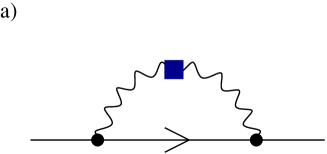
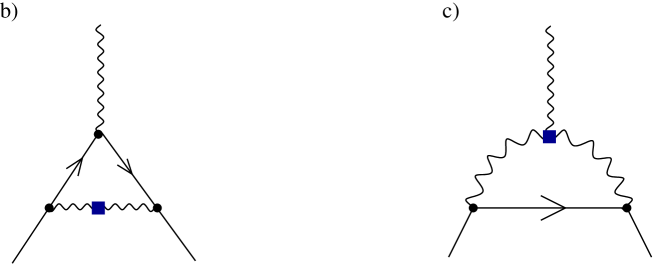
Figure 6: Soft dense loop contribution to the quark self energy (Fig. a)) and the quark-gluon vertex function (Figs. b) and c)). The solid squares denote the HDL gluon self energy and three-point function.

We saw that in the hard dense loop approximation the abelian and non-abelian vertex corrections are identical up to a color factor. The sum of the color factors of the two diagrams is $C^{(ab)}+C^{(nab)}=(C_{F}-C_{A}/2)+C_{A}/2=C_{F}$ which shows that the quark-gluon vertex in the HDL approximation has the same color structure as the quark self energy. The same result is also obtained for the leading IR divergence in the soft dense loop limit. The only difference is that following the arguments given above we have to take into account both the HDL gluon self energy and the HDL gluon three-point function when evaluating the non-abelian vertex function, see Fig. 6c. Indeed, the free gluon three-point function does not contribute to the IR divergence of the quark-gluon vertex in the SDL limit. We have

$$\Gamma^{(nab)}_{\alpha}(p_{1},p_{2}) = g^{3}C^{(nab)}\int\frac{d^{4}k}{(2\pi)^{4}}v_{\mu}v_{\nu}D_{\mu\mu^{\prime}}(k)\Gamma_{\alpha\mu^{\prime}\nu^{\prime}}(p_{2}-p_{1},k,p_{1}-p_{2}-k)$$ (44)

$$\hskip 56.9055pt\cdot D_{\nu^{\prime}\nu}(p_{1}-p_{2}-k)\frac{1}{(p_{1})_{0}-k_{0}-l_{p_{1}-k}}.$$

Again the interesting limit is $(l_{p_{1}}-l_{p_{2}})\ll(p_{1}-p_{2})_{4}$. The calculation is greatly simplified by the observation that in this limit equ. (29) gives

$$\Gamma_{4\mu\nu}(p_{2}-p_{1},k,p_{1}-p_{2}-k) \simeq \frac{1}{(p_{2}-p_{1})_{4}}\left\{\Pi_{\mu\nu}(k+(p_{2}-p_{1}))-\Pi_{\mu\nu}(k)\right\}$$ (45)

$$\simeq \frac{\partial}{\partial p_{4}}\Pi_{\mu\nu}(k+p)\simeq P^{T}_{\mu\nu}\frac{\partial}{\partial p_{4}}\Pi_{M}(k+p).$$

This relation is also a direct consequence of the Ward identity for the HDL gluon three-point function. Using equ. (45) and continuing to euclidean space we get the following expression for the non-abelian vertex function in the limit $(l_{p_{1}}-l_{p_{2}})\ll(p_{1}-p_{2})_{4}$

$$\Gamma^{(nab)}_{\alpha}(p)=g^{3}C^{(nab)}v_{\alpha}\int\frac{dl_{4}}{2\pi}\int\frac{l^{2}dl}{4\pi^{2}}\int dx\,\frac{1-x^{2}}{[l_{4}^{2}+l^{2}+\frac{\pi}{2}m^{2}\frac{l_{4}}{l}]^{2}}\frac{\pi}{2}m^{2}\frac{1}{l}\frac{1}{i(l_{4}+p_{4})-lx}.$$ (46)

This integral can be evaluated using the same strategy as for the abelian vertex. First we observe that to leading logarithmic accuracy we can replace $(1-x^{2})\to 1$. The integral over $x$ then gives

$$\int dx\,\frac{1}{i(l_{4}+p_{4})-lx}=\frac{2i}{l}\arctan\left(\frac{l}{l_{4}+p_{4}}\right).$$ (47)

In the limit $p_{4}\to 0$ the integral over $l_{4}$ is dominated by the discontinuity of the inverse tan function and

$$\lim_{(p_{1})_{4}\to(p_{2})_{4}}\lim_{l_{p_{1}}\to l_{p_{2}}}\Gamma^{(nab)}_{\alpha}(p_{1},p_{2})=\frac{g^{3}C^{(nab)}v_{\alpha}}{12\pi^{2}}\log\left(\frac{\Lambda}{p_{4}}\right).$$ (48)

The non-abelian vertex function in the limit $(l_{p_{1}}-l_{p_{2}})\gg(p_{1}-p_{2})_{4}$ can be computed using the same methods. We find that there is no logarithmic enhancement near the Fermi surface. We conclude that the abelian and non-abelian soft dense loop vertex functions have the same logarithmic singularity and that the sum of the two contributions is proportional to $C^{(ab)}+C^{(nab)}=C_{F}$.

VI Color Superconductivity

Soft dense loop corrections to the fermion self energy and the quark-gluon vertex function become comparable to the free propagator and the free vertex at the scale $E\sim\mu\exp(-1/g^{2})$. This implies that at this scale soft dense loops have to be resummed. Physically, this resummation corresponds to the study of non-Fermi liquid effects in dense quark matter Boyanovsky:2000bc . However, before non-Fermi liquid effects become important the quark-quark interaction in the BCS channel becomes singular. The scale of superfluidity is $E\sim\mu\exp(-1/g)$ Son:1999uk . This scale is smaller than the HDL scale but larger than the SDL scale. This implies that we have to resum quark-quark scattering with HDL dressed gluon propagators but that SDL corrections to the quark self energy and the quark-gluon vertex are small and can be treated perturbatively.

The resummation of the quark-quark scattering amplitude in the BCS channel leads to the formation of a non-zero gap in the single particle spectrum. We can take this effect into account in the high density effective theory by including a tree level gap term

$${\cal L}=\Delta\,R_{l}^{\Gamma}(\vec{v}\cdot\hat{\Delta})\psi_{-v}\sigma_{2}\Gamma\psi_{v}+h.c..$$ (49)

Here, $\Gamma$ is any of the helicity structures introduced in Sect. III, $R_{l}^{\Gamma}(x)$ is the corresponding angular factor and $\hat{\Delta}$ is a unit vector. The magnitude of the gap is determined variationally, by requiring the free energy to be stationary order by order in perturbation theory. We shall see that the gap varies with the energy or the residual momentum on a scale set by the gap itself. As a result the energy dependence is relevant and we cannot replace the gap by its value on the Fermi surface. In order to do perturbation theory in the presence of a gap term we will use the Nambu-Gorkov method and introduce a two component field $\Psi=(\psi_{v},\psi^{\dagger}_{-v}\sigma_{2})$. The inverse propagator for the field $\Psi$ is

$$S^{-1}(p)=\left(\begin{array}[]{cc}v\cdot p&\Delta(p)R_{l}^{\Gamma}(\vec{v}\cdot\hat{\Delta})\Gamma\\ \Delta^{*}(p)R_{l}^{\Gamma}(\vec{v}\cdot\hat{\Delta})\Gamma^{\dagger}&\bar{v}\cdot p\end{array}\right),$$ (50)

where $\bar{v}_{\mu}=(1,-\vec{v})$. The variational principle for the gap $\Delta$ gives the Dyson-Schwinger equation

$$\Delta(p_{4})=\frac{2g^{2}}{3}\int\frac{d^{4}q}{(2\pi)^{4}}\frac{\Delta(q_{4})}{q_{4}^{2}+l_{q}^{2}+\Delta(q_{4})^{2}}v_{\mu}v_{\nu}D_{\mu\nu}(p-q),$$ (51)

where the factor in front of the integral is the color factor corresponding to the color anti-symmetric $[\bar{3}]$ channel. It is sufficient to solve this equation to leading logarithmic accuracy. We shall see in the next section that corrections to the gap can be computed perturbatively, without solving the gap equation to higher accuracy. To leading logarithmic accuracy the gap equation is dominated by the IR divergence in the magnetic gluon propagator. This IR divergence is independent of the helicity and angular momentum channel. We have

$$\Delta(p_{4})=\frac{g^{2}}{18\pi^{2}}\int_{0}^{\Lambda_{\|}}dq_{4}\frac{\Delta(q_{4})}{\sqrt{q_{4}^{2}+\Delta(q_{4})^{2}}}\log\left(\frac{\Lambda_{\perp}}{|p_{4}^{2}-q_{4}^{2}|^{1/2}}\right).$$ (52)

The leading logarithmic behavior is independent of the ratio of the cutoffs and we can set $\Lambda_{\|}=\Lambda_{\perp}=\Lambda$. We introduce the dimensionless variables variables $x=\log(2\Lambda/(q_{4}+\epsilon_{q}))$ and $y=\log(2\Lambda/(p_{4}+\epsilon_{p})$ where $\epsilon_{q}=(q_{4}^{2}+\Delta(q_{4}))^{1/2}$. In terms of dimensionless variables the gap equation is given by

$$\Delta(y)=\frac{g^{2}}{18\pi^{2}}\int_{0}^{x_{0}}dx\,\Delta(x)K(x,y),$$ (53)

where $x_{0}=\log(2\Lambda/\Delta_{0})$ and $K(x,y)$ is the kernel of the integral equation. At leading order we can use the approximation $K(x,y)=\min(x,y)$ Son:1999uk . We can perform an additional rescaling $x=x_{0}\bar{x}$, $y=x_{0}\bar{y}$. Since the leading order kernel is homogeneous in $x,y$ we can write the gap equation as an eigenvalue equation

$$\Delta(\bar{y})=x_{0}^{2}\frac{g^{2}}{18\pi^{2}}\int_{0}^{1}d\bar{x}\,\Delta(\bar{x})K(\bar{x},\bar{y}),$$ (54)

where the gap function is subject to the boundary conditions $\Delta(0)=0$ and $\Delta^{\prime}(1)=0$. Son observed that equ. (54) is equivalent to the differential equation Son:1999uk

$$\Delta^{\prime\prime}(\bar{x})=-x_{0}^{2}\left(\frac{g^{2}}{18\pi^{2}}\right)\Delta(\bar{x}),$$ (55)

which has the solutions

$$\Delta_{n}(\bar{x})=\Delta_{n,0}\sin\left(\frac{g}{3\sqrt{2}\pi}x_{0,n}\bar{x}\right),\hskip 28.45274ptx_{0,n}=(2n+1)\frac{3\pi^{2}}{\sqrt{2}g}.$$ (56)

The physical solution corresponds to $n=0$ which gives the largest gap, $\Delta_{0}=2\Lambda\exp(-3\pi^{2}/(\sqrt{2}g))$. Solutions with $n\neq 0$ have smaller gaps and are not global minima of the free energy.

VII Perturbative corrections to the gap parameter

The complete set of solutions of the leading order gap equation can be used to set up a perturbative scheme for computing corrections to the gap function. This perturbative scheme is similar to the one used by Brown et al. in order to compute corrections to the critical temperature Brown:1999yd . We first observe that the functions $\Delta_{n}(\bar{x})$ form an orthogonal set of solutions of the gap equation

$$\int_{0}^{1}d\bar{x}\,\Delta_{n}(\bar{x})\Delta_{m}(\bar{x})=\delta_{m,n}.$$ (57)

We now consider the gap equation with the kernel $K(x,y)+\delta K(x,y)$ where $K(x,y)$ contains the leading IR divergence and $\delta K(x,y)$ is a perturbative correction. We have

$$\Delta(\bar{y})=x_{0}^{2}\frac{g^{2}}{18\pi^{2}}\int_{0}^{1}d\bar{x}\,\Delta(\bar{x})K(\bar{x},\bar{y})+x_{0}\frac{g^{2}}{18\pi^{2}}\int_{0}^{1}d\bar{x}\,\Delta(\bar{x})\delta K(x_{0}\bar{x},x_{0}\bar{y}).$$ (58)

We write the gap function $\Delta(\bar{x})$ and the eigenvalue $x_{0}$ as a perturbative expansion in $\delta K$

$$\Delta(\bar{x}) = \Delta^{(0)}(\bar{x})+\Delta^{(1)}(\bar{x})+\Delta^{(2)}(\bar{x})+\ldots,$$ (59)

$$x_{0} = x_{0}^{(0)}+x_{0}^{(1)}+x_{0}^{(2)}+\ldots.$$ (60)

Using the orthogonality of the unperturbed solutions $\Delta_{n}(\bar{x})$ we can derive expressions for $\Delta^{(i)}$ and $x_{0}^{(i)}$. These expressions are very similar to ordinary Rayleigh-Schroedinger perturbation theory. At first order in perturbation theory we get

$$x_{0}^{(1)}=-\frac{1}{2}\left(x_{0}^{(0)}\right)^{2}\frac{g^{2}}{18\pi^{2}}\int_{0}^{1}d\bar{x}\int_{0}^{1}d\bar{y}\,\Delta_{0}^{(0)}(\bar{x})\delta K(x_{0}\bar{x},x_{0}\bar{y})\Delta_{0}^{(0)}(\bar{y}),$$ (61)

and

$$c^{(1)}_{k}=\frac{1}{1-\left(\frac{1}{2k+1}\right)^{2}}\,x_{0}^{(0)}\frac{g^{2}}{18\pi^{2}}\int_{0}^{1}d\bar{x}\int_{0}^{1}d\bar{y}\,\Delta^{(0)}_{0}(\bar{x})\delta K(x_{0}\bar{x},x_{0}\bar{y})\Delta^{(0)}_{k}(\bar{y}),$$ (62)

where $c_{k}^{(1)}$ are the components of $\Delta^{(1)}(\bar{x})$ in the basis of the unperturbed gap functions, $\Delta^{(1)}(\bar{x})=\sum c^{(1)}_{k}\Delta^{(0)}_{k}(\bar{x})$. Equ. (61) shows that the first order correction to the pairing gap can be computed using the unperturbed gap function.

The simplest example for a correction to the kernel is is a contact term

$$\delta K(x_{0}\bar{x},x_{0}\bar{y})=\log(b).$$ (63)

In Sect. VIII we will show that the coefficient $b$ is determined by four-fermion operators in the effective theory. The unperturbed gap is given by $\Delta=\Lambda\exp(-x^{(0)}_{0})=\Lambda\exp(-3\pi^{2}/(\sqrt{2}g))$. Using equ. (61) and equ. (63) we get

$$\Delta=\Lambda e^{-(x^{(0)}_{0}+x^{(1)}_{0}+\ldots)}=b\Lambda e^{-\frac{3\pi^{2}}{\sqrt{2}g}}.$$ (64)

We conclude that contact terms modify the prefactor of the gap. We also notice that because of the orthogonality of the gap functions a contact term does not modify the shape of the gap function.

We can also study the effect of the quark self energy Brown:1999aq ; Wang:2001aq . Equ. (38) implies a wave function renormalization

$$Z(p_{4})=1-\frac{g^{2}C_{F}}{12\pi^{2}}\log\left(\frac{\Lambda}{p_{4}}\right).$$ (65)

The corresponding correction to the kernel of the gap equation is

$$\delta K(x_{0}\bar{x},x_{0}\bar{y})=-\frac{g^{2}}{9\pi^{2}}\left(x_{0}\bar{x}\right)K(x_{0}\bar{x},x_{0}\bar{y}),$$ (66)

where we have used $C_{F}=4/3$ for $N_{c}=3$ and $K(x,y)=\min(x,y)$ is the leading order kernel. Using equ. (61) we find

$$x^{(1)}_{0} = \frac{1}{2}\left(x_{0}^{(0)}\right)^{2}\frac{g^{2}}{18\pi^{2}}\int_{0}^{1}d\bar{x}\int_{0}^{1}d\bar{y}\,\frac{g^{2}}{9\pi^{2}}(x_{0}\bar{x})\Delta^{(0)}_{0}(\bar{x})K(x_{0}\bar{x},x_{0}\bar{y})\Delta^{(0)}_{0}(\bar{y})$$ (67)

$$= \frac{1}{2}\frac{g^{2}}{9\pi^{2}}\left(x_{0}^{(0)}\right)^{2}\int_{0}^{1}d\bar{x}\,\bar{x}\left[\Delta^{(0)}_{0}(\bar{x})\right]^{2}=\frac{4+\pi^{2}}{8},$$

where we have used the fact that $\Delta^{(0)}_{0}(\bar{x})$ is an eigenfunction of the unperturbed kernel. The result equ. (67) corresponds to a reduction of the gap by a factor $\exp(-(4+\pi^{2})/8)$. We can also see that the fermion self energy correction leads to an admixture of higher harmonics of the gap function. However, these admixtures are small, $c_{k}^{(1)}=O(g)$, for all values of $k$.

There is a slight subtlety with regard to the result equ. (67). In section V we computed the wave function renormalization in the normal phase. We observed, however, that the scale of non-Fermi liquid effects, $E\sim\mu\exp(-1/g^{2})$, is exponentially small as compared to the scale where pairing sets in, $E\sim\mu\exp(-1/g)$. This implies that also the normal component of the fermion self energy should be computed with the gap taken into account. It is easy to see that in this case equ. (38) is modified to

$$\Sigma(p_{4})\simeq\frac{g^{2}C_{F}}{12\pi^{2}}p_{4}\log\left(\frac{\Lambda}{\sqrt{p_{4}^{2}+\Delta^{2}}}\right).$$ (68)

Pairing removes the infrared divergence in the wave function renormalization. However, in the superfluid phase the fermion self energy is only modified for very small energies $p_{4}<\Delta$ whereas the correction to the gap is dominated by the regime $p_{4}>\Delta$. As a consequence the result equ. (67) is not changed. Finally, we have to consider the role of soft dense loop vertex corrections given in equ. (43) and (48). The infrared logarithm in the vertex correction only appears in the regime $|l_{p}-l_{q}|\ll|p_{4}-q_{4}|$. Since the gap equation determines the anomalous self energy on the quasi-particle mass shell, $p_{4}\simeq(l_{q}^{2}+\Delta^{2})^{1/2}$, this implies that $l_{q}\ll q_{4}$. However, this condition eliminates the BCS logarithm in the gap equation (51). As a consequence, the infrared logarithm in the quark-gluon vertex does not modify the eigenvalue $x_{0}$ at $O(1)$ in the coupling constant. Vertex corrections to the gap equation were first considered in Schafer:1999jg but the arguments given in that work are not correct. A more detailed study can be found in Brown:2000eh .

VIII Matching contact terms

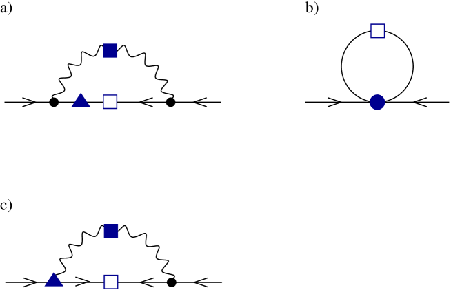
Figure 8: Corrections to the gap equation. Fig. a) shows the soft dense loop quark self energy correction, Fig. b) local four-fermion interactions, and Fig. c) shows the soft dense loop vertex correction. The solid triangles denote the SDL self energy and vertex correction and the solid circle is the four-fermion interaction in the effective theory.

Consider the effect of the $O(1/\mu^{2})$ contact term equ. (21) on the pairing gap. The contribution of this term to the kernel of the gap equation involves a sum over patches, see Fig. 8. As a consequence the correction to the kernel, $g^{2}\delta K(x,y)=6V_{0}^{++}$, is not suppressed by $1/\mu^{2}$. In the previous section we showed that $O(g^{2})$ constants in the kernel contribute to the eigenvalue at $O(1)$. This implies that we have to determine to coefficients of $O(g^{2}/\mu^{2})$ contact terms in the high density effective theory in order to determine the eigenvalue of the gap equation to $O(1)$.

This can be achieved by matching the quark-quark scattering amplitude in the BCS channel. The tree level scattering amplitude in the spin zero color anti-triplet channel is given by

$$f(\theta)=\frac{2g^{2}}{3}\left\{\frac{\frac{1}{2}(1+\cos\theta)}{2\mu^{2}(1-\cos\theta)+\Pi_{E}}+\frac{\frac{1}{2}(3-\cos\theta)}{2\mu^{2}(1-\cos\theta)+\Pi_{M}}\right\}.$$ (69)

At leading order in the effective theory this amplitude is represented by

$$f_{HDET}(\theta) = \frac{2g^{2}}{3}\left.\left\{\frac{1}{2\mu^{2}(1-\cos\theta)+\Pi_{E}}+\frac{1}{2\mu^{2}(1-\cos\theta)+\Pi_{M}}\right\}\right|_{1-\cos\theta<\Lambda_{\perp}^{2}/(2\mu^{2})}$$ (70)

$$\hskip 28.45274pt\mbox{}+\frac{V^{++}_{l}(\Lambda_{\perp})}{\mu^{2}}P_{l}(\cos\theta),$$

where the collinear term is cut off at $l_{\perp}^{2}=\Lambda_{\perp}^{2}$. The matching condition requires that the partial wave amplitudes corresponding to equ. (69) and (70) are the same. Since the collinear term in the high density effective theory is regulated by a UV cutoff the counterterm depends on the cutoff, too. The matching condition is simplest for $\Lambda_{\perp}^{2}=2\mu^{2}$. The s-wave term is given by

$$V^{++}_{0}(2\mu^{2})=\frac{2g^{2}}{3}\frac{1}{4}\int_{-1}^{1}dx\,\left\{\frac{-\frac{1}{2}(1-x)}{(1-x)+\Pi_{E}/(2\mu^{2})}+\frac{\frac{1}{2}(1-x)}{(1-x)+\Pi_{M}/(2\mu^{2})}\right\}=0,$$ (71)

up to corrections of $O(g^{4})$. The cutoff dependence of $V_{0}^{++}$ is controlled by the renormalization group equation

$$\Lambda_{\perp}^{2}\frac{d}{d\Lambda_{\perp}^{2}}V_{0}^{++}(\Lambda_{\perp}^{2})=\frac{g^{2}}{3}.$$ (72)

This equation implies that the kernel in the gap equation is independent of the cutoff $\Lambda_{\perp}$. We find Schafer:1999jg ; Hong:2000fh ; Pisarski:2000tv

$$K(p_{4},q_{4})=\log\left(\frac{\Lambda_{\perp}}{|p_{4}^{2}-q_{4}^{2}|^{1/2}}\right)+\log\left(\frac{512\pi^{4}\mu}{g^{5}\Lambda_{\perp}}\left(\frac{2}{N_{f}}\right)^{\frac{5}{2}}\right).$$ (73)

Using the leading order result equ. (56), the perturbative corrections equ. (64,67), and the value of the counterterm given in equ. (73) we get the standard result for the gap in the 2SC phase

$$\Delta=512\pi^{4}(2/N_{f})^{5/2}\mu g^{-5}e^{-\frac{4+\pi^{2}}{8}}e^{-\frac{3\pi^{2}}{\sqrt{2}g}}.$$ (74)

Note that at this order we did not have to fix the dependence of the counterterms on the longitudinal cutoff $\Lambda_{\|}$.

We saw that $V_{0}^{++}(2\mu^{2})$ vanishes to leading order in perturbation theory. This is not the case for higher partial wave terms and operators with non-zero spin. For example, the total angular momentum one counter term in the total helicity zero channel is

$$V^{++}_{1}(2\mu^{2})=\frac{2g^{2}}{3}\frac{3}{4}\int_{-1}^{1}dx\,\frac{x[(\frac{1}{2}+\frac{x}{2})+(\frac{3}{2}-\frac{x}{2})]-2}{1-x}=-6\frac{g^{2}}{3}.$$ (75)

The tree level matrix element in the helicity one channel is proportional to $(1+\cos\theta)/2$ for both electric and magnetic gluon exchanges. The corresponding counterterm is

$$V^{+-}_{1}(2\mu^{2})=\frac{2g^{2}}{3}\frac{3}{4}\int_{-1}^{1}dx\,\frac{d^{(1)}_{11}(x)[(\frac{1}{2}+\frac{x}{2})+(\frac{1}{2}+\frac{x}{2})]-2}{1-x}=-\frac{9}{2}\frac{2g^{2}}{3},$$ (76)

where we have used $d^{(1)}_{11}(x)=(1+x)/2$. These results imply that the total angular momentum one gaps are given by $\Delta^{++}_{1}=\exp(-6)\Delta^{++}_{0}$ and $\Delta^{+-}_{1}=\exp(-9/2)\Delta^{++}_{0}$ where $\Delta^{++}_{0}$ is the s-wave gap given in equ. (74) Brown:1999yd ; Schafer:2000tw ; Schmitt:2002sc .

IX Summary

In this work we studied several problems related to the use of effective field theories in QCD at large baryon density. We showed that the power counting in $1/\mu$ is complicated by the appearance of two scales inside loop integrals. Hard dense loops involve the large scale $\mu^{2}$ and lead to phenomena such as screening and damping at the scale $g\mu$. Soft loops only involve small scales and lead to superfluidity and non-Fermi liquid behavior at exponentially small scales. We also showed that contact terms in the effective lagrangian are suppressed by powers of $1/\mu^{2}$, but they get enhanced by hard loops. As a result contact terms contribute to the pre-exponent of the pairing gap at $O(1)$. We performed the necessary matching calculation to determine four-fermion operators in the effective theory.

There are many problems that remain to be studied. We would like to understand not only how to count powers of $E/\mu$ but also logarithms. This is essential for understanding the structure of the expansion of the gap and other quantities in the coupling constant. Another issue is the choice of regularization scheme. In this work we have used a momentum space cutoff throughout. There are, however, some HDET calculations that have been performed using dimensional regularization. It is clearly important to understand the power counting in both schemes.

We would also like to have a better understanding of gauge invariance. The high density effective theory has the advantage that the pre-exponent of the gap is determined by counterterms that are matched against on-shell scattering amplitudes and that are therefore manifestly gauge invariant. This result agrees with explicit calculations in a generalized Coulomb gauge Pisarski:2001af but not with calculations in a general covariant gauge Hong:2000fh . A formal argument that the full quasi-particle propagator is gauge invariant was recently presented in Gerhold:2003js . It is well known that the hard dense loop effective action equ. (31) is gauge invariant. It is not clear whether there is a similar statement for soft dense loops. Brown et al. showed that the soft quark self energy and quark gluon vertex function satisfy BRST identities Brown:2000eh . We have also checked that the IR divergences in the soft wave function renormalization and vertex are independent of the gauge parameter in a general Coulomb gauge. On the other hand, Hsu et al. have argued that one can find a non-local gauge in which there is no wave function renormalization Hong:2003ts .

Hong and Hsu have argued that the high density effective theory can be formulated non-perturbatively, using a lattice regulator, and that the leading order theory has a positive euclidean measure Hong:2002nn . Such a formulation might be useful in order to study certain non-perturbative questions and to provide guidance in the search for algorithms capable of simulating gauge theories at non-zero baryon density. Our results suggest, however, that there are some difficulties with this proposal. The leading order effective theory is defined on a single patch, or, if a gap term is added, on two patches corresponding to Fermi velocities $\pm\vec{v}$. In this theory the ground state is likely a coherent particle-hole state of the type suggested by Deryagin, Grigoriev and Rubakov Deryagin:rw . The reason is that the forward scattering amplitude in the particle-hole channel is larger than the one in the particle-particle channel. This state is disfavored in the full theory, because the corresponding four-fermion operator is not enhanced by hard dense loops. This means that operators that are superficially sub-leading are important in selecting the correct ground state. Physically, this is related to the fact that the particle-hole state can only become coherent over the entire Fermi surface if the surface is nested, but not if the Fermi surface is spherical. Another problem is how to correctly incorporate the boundary conditions for the effective theory. The lagrangian of the leading order theory is equal to the non-relativistic QCD (NRQCD) lagrangian. However, the physics of the high density theory and NRQCD are very different. For example, there is no screening in the gluon two-point function in NRQCD. This issue is also related to the necessity to add a two-gluon counterterm to the effective theory. In perturbation theory this difference is encoded in different $i\epsilon$ prescriptions for the fermion propagator. It would be interesting to understand how the boundary conditions are realized on a euclidean lattice. Some of these issues are studied in Hong:2003zq .

Acknowledgments: We would like to thank S. Beane, P. Bedaque, and D. Rischke for useful discussions. This work was supported in part by US DOE OJI grant and by US DOE grant DE-FG-88ER40388.

Figure 1: Hard dense loop contributions to the the gluon and quark self energy. Fig a) shows the particle-hole contribution to the gluon self energy, b) shows the anti-particle contribution, and c) shows the quark self energy.

Figure 2: Hard dense loop contributions to the gluon three and four function.

Figure 3: Hard dense loop contribution to the quark-gluon vertex function. Figure a) shows the abelian vertex and figure b) the non-abelian vertex.

Figure 5: Scales of the high density effective field theory.

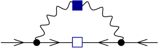
Figure 7: Leading order gap equation for the superconducting gap in the high density effective theory. The solid square denotes the HDL self energy and the open square is the anomalous quark self energy.

References

- (1) D. Bailin and A. Love, Phys. Rept. 107, 325 (1984).
- (2) M. Alford, K. Rajagopal and F. Wilczek, Phys. Lett. B422, 247 (1998) [hep-ph/9711395].
- (3) R. Rapp, T. Schäfer, E. V. Shuryak and M. Velkovsky, Phys. Rev. Lett. 81, 53 (1998) [hep-ph/9711396].
- (4) M. Alford, K. Rajagopal and F. Wilczek, Nucl. Phys. B537, 443 (1999) [hep-ph/9804403].
- (5) K. Rajagopal and F. Wilczek, The condensed matter physics of QCD, in: Festschrift in honor of B.L. Ioffe, ’At the Frontier of Particle Physics / Handbook of QCD’, M. Shifman, ed., World Scientific, Singapore, hep-ph/0011333.
- (6) M. Alford, Ann. Rev. Nucl. Part. Sci. 51, 131 (2001) [hep-ph/0102047].
- (7) T. Schäfer, Quark Matter, BARC workshop on Quarks and Mesons; to appear in the proceedings, hep-ph/0304281.
- (8) D. H. Rischke, The Quark-Gluon Plasma in Equilibrium, to appear in Prog. Part. Nucl. Phys, nucl-th/0305030.
- (9) S. Reddy, Acta Phys. Polon. B 33, 4101 (2002) [nucl-th/0211045].
- (10) M. Alford, Lect. Notes Phys. 583, 81 (2002).
- (11) T. Schäfer and F. Wilczek, Phys. Rev. Lett. 82, 3956 (1999) [hep-ph/9811473].
- (12) M. Gell-Mann, K. Brueckner, Phys. Rev. 106, 364 (1957).
- (13) T. Holstein, A. E. Norton, P. Pincus, Phys. Rev. B8, 2649 (1973).
- (14) M. Yu. Reizer, Phys. Rev. B 40, 11571 (1989).
- (15) D. K. Hong, Phys. Lett. B 473, 118 (2000) [hep-ph/9812510].
- (16) D. K. Hong, Nucl. Phys. B 582, 451 (2000) [hep-ph/9905523].
- (17) S. R. Beane and P. F. Bedaque, Phys. Rev. D 62, 117502 (2000) [nucl-th/0005052].
- (18) S. R. Beane, P. F. Bedaque and M. J. Savage, Phys. Lett. B 483, 131 (2000) [hep-ph/0002209].
- (19) T. Schäfer, Phys. Rev. D 65, 074006 (2002) [hep-ph/0109052].
- (20) R. Casalbuoni, R. Gatto, M. Mannarelli and G. Nardulli, Phys. Lett. B 524, 144 (2002) [hep-ph/0107024].
- (21) G. Nardulli, Riv. Nuovo Cim. 25N3, 1 (2002) [hep-ph/0202037].
- (22) E. Braaten and R. D. Pisarski, Nucl. Phys. B 337, 569 (1990).
- (23) J. P. Blaizot and J. Y. Ollitrault, Phys. Rev. D 48, 1390 (1993) [hep-th/9303070].
- (24) C. Manuel, Phys. Rev. D 53, 5866 (1996) [hep-ph/9512365].
- (25) D. H. Rischke, Phys. Rev. D 62, 034007 (2000) [nucl-th/0001040].
- (26) T. Schäfer and F. Wilczek, Phys. Lett. B450, 325 (1999) [hep-ph/9810509].
- (27) T. Schäfer, Phys. Rev. D 65, 094033 (2002) [hep-ph/0201189].
- (28) M. Jacob and G. C. Wick, Annals Phys. 7, 404 (1959) [Annals Phys. 281, 774 (2000)].
- (29) E. Braaten and R. D. Pisarski, Phys. Rev. D 45, 1827 (1992).
- (30) E. Braaten, Can. J. Phys. 71, 215 (1993) [hep-ph/9303261].
- (31) W. E. Brown, J. T. Liu and H. c. Ren, Phys. Rev. D 62, 054016 (2000) [hep-ph/9912409].
- (32) W. E. Brown, J. T. Liu and H. c. Ren, Phys. Rev. D 62, 054013 (2000) [hep-ph/0003199].
- (33) D. Boyanovsky and H. J. de Vega, Phys. Rev. D 63, 034016 (2001) [hep-ph/0009172].
- (34) C. Manuel, Phys. Rev. D 62, 114008 (2000) [hep-ph/0006106].
- (35) B. Vanderheyden and J. Y. Ollitrault, Phys. Rev. D 56, 5108 (1997) [hep-ph/9611415].
- (36) D. T. Son, Phys. Rev. D 59, 094019 (1999) [hep-ph/9812287].
- (37) W. E. Brown, J. T. Liu and H. Ren, Phys. Rev. D61, 114012 (2000) [hep-ph/9908248].
- (38) Q. Wang and D. H. Rischke, Phys. Rev. D 65, 054005 (2002) [nucl-th/0110016].
- (39) T. Schäfer and F. Wilczek, Phys. Rev. D60, 114033 (1999) [hep-ph/9906512].
- (40) D. K. Hong, V. A. Miransky, I. A. Shovkovy and L. C. Wijewardhana, Phys. Rev. D61, 056001 (2000) [hep-ph/9906478].
- (41) R. D. Pisarski and D. H. Rischke, Phys. Rev. D61, 074017 (2000) [nucl-th/9910056].
- (42) T. Schäfer, Phys. Rev. D 62, 094007 (2000) [hep-ph/0006034].
- (43) A. Schmitt, Q. Wang and D. H. Rischke, Phys. Rev. D 66, 114010 (2002) [nucl-th/0209050].
- (44) R. D. Pisarski and D. H. Rischke, Nucl. Phys. A 702, 177 (2002) [nucl-th/0111070].
- (45) A. Gerhold and A. Rebhan, preprint, hep-ph/0305108.
- (46) D. K. Hong, T. Lee, D. P. Min, D. Seo and C. Song, preprint, hep-ph/0303181.
- (47) D. K. Hong and S. D. Hsu, Phys. Rev. D 66, 071501 (2002) [hep-ph/0202236].
- (48) D. V. Deryagin, D. Y. Grigoriev and V. A. Rubakov, Int. J. Mod. Phys. A 7, 659 (1992).
- (49) D. K. Hong and S. D. Hsu, preprint, hep-ph/0304156.