Excited nucleons with chirally improved fermions

Abstract

We study positive and negative parity nucleons on the lattice using the chirally improved lattice Dirac operator. Our analysis is based on a set of three operators $\chi_{i}$ with the nucleon quantum numbers but in different representations of the chiral group and with different diquark content. We use a variational method to separate ground state and excited states and determine the mixing coefficients for the optimal nucleon operators in terms of the $\chi_{i}$. We clearly identify the negative parity resonances $N(1535)$ and $N(1650)$ and their masses agree well with experimental data. The mass of the observed excited positive parity state is too high to be interpreted as the Roper state. Our results for the mixing coefficients indicate that chiral symmetry is important for $N(1535)$ and $N(1650)$ states. We confront our data for the mixing coefficients with quark models and provide insights into the physics of the nucleon system and the nature of strong decays.

I Introduction

Lattice QCD has the potential to answer some of the most important questions about the proper effective degrees of freedom in the nucleon and its excitations. In particular, one is able to arbitrarily change the mass of quarks and hence to study the evolution of nucleon properties such as its mass and excitation spectrum as a function of the current quark mass. This is interesting because we know the physical picture which drives hadrons made of heavy quarks. In this case the hadrons can be well approximated by the non-relativistic QCD picture, where the most important ingredients are the linear + Coulomb potential as well as a hyperfine correction that originates from the perturbative color-magnetic interaction between spins of heavy quarks.

The most prominent implication of this picture is the structure of the heavy quarkonium spectrum. The color-magnetic spin-spin force induces a splitting between the ${}^{3}S_{1}$ and ${}^{1}S_{0}$ ground states. The linear + Coulomb interaction drives the pattern of radially and orbitally excited states: The first orbital excitation which carries $L=1$ orbital angular momentum and has a parity which is opposite to the given ground state, lies always below the first radial excitation, which has the same quantum numbers as the ground state. Such a pattern is quantitatively understood within non-relativistic lattice QCD as well as the potential approach (for a review and references see e.g. Ref. D ).

On the other hand the ordering of the lowest positive and negative parity excitations of the nucleon is just opposite. The first radial excitation of the nucleon, the Roper resonance $1/2^{+}$, $N(1440)$, lies about 100 MeV below the first orbital excitation, $1/2^{-}$, $N(1535)$. A similar pattern is observed in the $\Delta$ spectrum, while the opposite ordering of the lowest positive-negative parity $J=1/2$ states takes place in the $\Lambda$ spectrum. It appears to be impossible to explain this within a linear confinement plus perturbative gluon exchange correction picture.

The whole experience of nuclear physics as well as numerous data on the chiral structure of the nucleon teach us that the consequences of spontaneous chiral symmetry breaking should be very important for the nucleon. A possible – certainly oversimplified – picture is that in the low energy regime the nucleon can be approximated as a system of three quasi-particles with dynamical mass induced by spontaneous chiral symmetry breaking (constituent quarks) which are confined. Such a picture is the most straightforward realization of the $SU(6)$ symmetry. The latter, in turn, can be proved to be an exact symmetry of QCD for ground state baryons in the large $N_{c}$ limit largeN . Then the question arises, what are the other residual interactions between the constituent quarks which break $SU(6)$ symmetry? The empirical ordering of positive and negative parity states is opposite in mesons and baryons which indicates that some physical aspects are different in these systems. An anomalous ordering in baryons was explained to be possibly due to a significant contribution of the residual interaction mediated by the chiral (Goldstone boson) field G . A meson-like exchange interaction between valence quarks is possible within the quenched approximation in baryons, and not possible in mesons.

Attempts to address these issues within the lattice formulation have begun only recently manycalcs ; blumetal ; parityminussplita ; parityminussplitb ; leeetal ; dongetal ; sasaki . Mainly the two interpolating fields $\chi_{1}$ and $\chi_{2}$ (for their definition see below) have been used in order to extract the ground state nucleon as well as the lowest excited states of both parities. The operator $\chi_{1}$ is known to couple well to the nucleon ground state and has been used in lattice calculations for more than 20 years. This operator also couples to the $J^{P}=1/2^{-}$ (negative parity) state. And indeed, the lowest $1/2^{-}$ state was established and has a tendency to approach the physical $N(1535)$ state for small quark mass. The authors of blumetal see no splitting between the lowest and the next excited negative parity state $J^{P}=1/2^{-}$ $N(1650)$, whereas such splitting is noticed in parityminussplita ; parityminussplitb .

The first excited positive parity $N(1440)$ Roper state has not been identified in lattice studies manycalcs ; blumetal ; parityminussplita ; parityminussplitb . Initial hopes that it would have a reasonable overlap with $\chi_{2}$ have been abandoned since the plateaus seen from the $\chi_{2}$ correlator come out consistently too high (close to 2 GeV) to be the Roper state.

Recently leeetal ; dongetal the Roper state has been observed and reordering of the levels, such that the excited positive parity state falls below the negative parity states taking place at pseudoscalar masses somewhere between 200 - 500 MeV, was obtained in leeetal ; dongetal ; sasaki using the $\chi_{1}$ interpolator. Both articles rely crucially on advanced fitting techniques, i.e. Bayesian priors.

Here we tackle the analysis of the nucleon system combining different powerful strategies. In addition to the operators $\chi_{1},\chi_{2}$ we use a third operator $\chi_{3}$ and compute all cross correlations. This correlation matrix is then analyzed using the variational method variation which allows for a separation of ground and excited states. Using more operators in the variational method allows the system to better select those combinations of interpolators which have optimal overlap with the physical states. The possibility of a reordering of the levels at small quark masses suggests to use a Dirac operator with good chirality which allows one to go to small quark masses. Here we work with the chirally improved Dirac operator chirimp . We perform a careful analysis of finite volume effects which is crucial in a study of excited nucleons with their extended wavefunctions.

From the variational technique one obtains also important information on the optimal operators which have maximal overlap with the physical states. This is interesting not only from a technical point of view but it also provides important insight into the physics of the nucleon system. We compute the mixing coefficients which relate our operators $\chi_{i}$ to the optimal operators, i.e. the coefficients which determine the operator content of the physical states. These mixing coefficients are then studied as a function of the quark mass and confronted with information from quark models. We discuss the physical implications of this comparison.

Our article is organized as follows: In the next section we collect information on the lattice calculation such as simulation details, the operators used, the variational technique and our fitting methods. In Section 3 we discuss the diquark content of our nucleon interpolators and their chiral properties. This is followed by two sections where we discuss our raw data and then present the results for the mass spectrum. In Section VI we determine the mixing coefficients, discuss their physical implications in Section VII and we end with conclusions in Section VIII.

II Lattice technology

For our quenched calculation we use uncorrelated configurations from the Lüscher-Weisz gauge action Luweact . We work on $16^{3}\times 32$ and $12^{3}\times 24$ lattices using 100 configurations for both volumes and gauge coupling constant $\beta_{LW}=7.9$. The lattice spacing is $a=0.15$ fm as determined from the Sommer parameter in scale . We remark that the scale from the Sommer parameter agrees well with a determination from hadronic input bgrlarge . This gives rise to spatial extensions of 2.4 fm, respectively 1.8 fm. Throughout this paper we use this scale where we give mass values in physical units.

The gauge field configurations were treated with one step of hypercubic blocking hypblocking . We use the recently developed Chirally Improved (CI) Dirac operator chirimp . The CI operator is a systematic expansion of a solution of the Ginsparg-Wilson relation GiWi82 and has very good chiral properties. In bgrlarge the residual quark mass for the $\beta_{LW}=7.9$ ensembles used here was computed from the chiral extrapolation of the pion mass and found to be $m_{res}=-0.0020(5)a^{-1}=-2.7(7)$ MeV. It was demonstrated bgrlarge ; boston that the CI operator allows simulations with pseudoscalar-mass to vector-mass ratios down to $m_{PS}/m_{V}$ = 0.28 at relatively small cost and that it has good scaling properties. It was found bgrlarge that for the nucleon the scaling dependence on $a$ is of the size of the statistical error. For the states we focus on here, i.e. the excited positive parity state and the negative parity states, we have larger errors and the effects of finite $a$ are negligible. We use Jacobi smeared sources jacobi with a width of about 0.7 fm. For the nucleon we find that the signal at small quark masses is enhanced when smearing also the sink. This allows to go deeper to the chiral limit, while at the larger quark masses we find exact agreement between the data from smeared and point-like sinks. Thus for the nucleon we use smeared sinks for all quark masses. All correlators were projected to zero momentum. The inversion of the Dirac operator was done with the BiCGstab multi-mass solver beat and we use several different values of the quark mass in the range between $a\,m_{q}=0.013$ ($m_{PS}=270$ MeV) and $a\,m_{q}=0.2$ ($m_{PS}=866$ MeV). A more detailed account of our setting is given in bgrlarge .

For the extraction of nucleon data we implement the following set of operators:

$$\chi_{1}(x) = \;\;\epsilon_{abc}\left[u_{a}^{T}(x)\,C\,\gamma_{5}\,d_{b}(x)\right]\,u_{c}(x)\;,$$ (1)

$$\chi_{2}(x) = \;\;\epsilon_{abc}\left[u_{a}^{T}(x)\,C\,d_{b}(x)\right]\,\gamma_{5}\,u_{c}(x)\;,$$ (2)

$$\chi_{3}(x) = i\,\epsilon_{abc}\left[u_{a}^{T}(x)\,C\,\gamma_{\mu}\gamma_{5}d_{b}(x)\right]u_{c}(x)\;.$$ (3)

$C$ is the charge conjugation matrix and $T$ denotes transposition. The color indices are $a,b,c$, while for the Dirac indices we use matrix/vector notation. For the interpolator $\chi_{3}$ we use only the time-like component. All three operators have the quantum numbers of the nucleon but correspond to different representations of the chiral group and contain different diquark fields in the brackets in Eqs. (1) - (3). Therefore one would expect that they couple differently to the given physical state. In the next section we will discuss in detail these representations, the quantum numbers of the diquark fields and their physical implications.

We use the variational technique variation and compute all cross correlations of our operators $\chi_{i}$ listed in Eq. (1) - (3):

$$M_{\;i,j}^{\pm}(t)=\Big{\langle}\;\mbox{Tr}\,\Big{[}\,P_{\pm}\chi_{i}(t)\ \chi_{j}(0)^{\dagger}\,\Big{]}\;\Big{\rangle}\;\;.$$ (4)

We explicitly project our correlators to definite parity by inserting the projectors $P^{\pm}=\frac{1}{2}[1\pm\gamma_{4}]$ and the trace in Eq. (4) is taken in Dirac space. Note that 4 is the euclidean time direction and $\gamma_{4}$ the corresponding element of the Clifford algebra. In the following we often omit the superscript $\pm$ for brevity. In order to extract the ground state and excited levels we first normalize the correlation matrix $M$ and construct $D(t)=M^{-1/2}(t_{0})M(t)M^{-1/2}(t_{0})$, where the position $t_{0}$ of the time slice chosen for the normalization can be used to optimize the signal. For all results presented here we have used $t_{0}=1$, which in our conventions corresponds to propagation distance 0. We discuss this choice in Sect.V.

Note that $M$ is a hermitian, positive definite matrix such that its inverse square root exists. We remark that this normalization is designed to reduce the error but a separation of ground and excited states can be obtained also without this normalization. Actually we find that in our case we could work almost equally well with the unnormalized matrix $M$. The second step is a diagonalization of the hermitian matrix $D(t)$ giving rise to three real eigenvalues $\lambda_{i}(t),i=1,2,3$. Applying the lemma proven in variation one finds

$$\lambda_{i}(t) = C_{i}\,\exp\left[-(t-t_{0})\,E_{i}\right]$$ (5)

$$\times\Big{[}1+{\cal O}\Big{(}\exp\left[-(t-t_{0})\Delta E_{i}\right]\Big{)}\Big{]}\;,$$

where $\Delta E_{i}$ is the difference of $E_{i}$ to the first omitted energy level, i.e. $\Delta E_{i}=|E_{i}-E_{4}|$. We remark that the form quoted in Eq. (5) is the expression for the positive parity states when using the matrix $M^{+}$, projected to positive parity. For fitting the negative parity states one has to time-reverse the correlators, i.e. replace $t$ by $T-t$, where $T$ denotes the temporal extension of the lattice. The eigenvalues from $M^{-}$ are related to the eigenvalues from $M^{+}$ by a minus sign and time reversal. We average our results from $M^{+}$ and $M^{-}$ after the necessary transformation to increase the statistics.

Eq. (5) makes clear the strength of the variational method: Each eigenvalue corresponds to a different energy level which dominates its exponential decay. For a large enough set of operators this allows for a clean separation of ground state and excited levels and we can apply a simple stable 2-parameter ($C_{i},\,E_{i}$) fit to determine the corresponding energy. In principle an $N\times N$ correlation matrix is sufficient for determining the ground state and the first $N-1$ excited states as long as the operators are linearly independent and each of the physical states has overlap with at least one operator. However, using more operators improves the results. The “perfect operator” has infinitely many different lattice operators (point split, different levels of smearing etc.). Some have large coefficients and others don’t. Selecting those with large overlap is a highly non-trivial task and requires in principle a knowledge of the wave function.

For a somewhat simpler problem - the application of the correlation matrix technique to a scattering problem - where there is a natural ordering of the operators (relative momenta of the scattering particles) a criterion to determine how many operators are needed was given in variationb .

Our $\chi^{2}$ functional uses the full correlation matrix. The fit ranges were determined from effective mass plateaus and we find values of $\chi^{2}/d.o.f.$ ranging from 0.5 to 1.5. Slight increases or decreases of the fit range leave our fit results and the $\chi^{2}/d.o.f.$ essentially invariant. We found that in the negative parity sector and for the excited positive parity state the quality of the data decreases for small quark masses and we could not maintain the standards of our fitting procedure. We do not give our results for these cases. The errors we quote were computed using jackknife subensembles.

III Diquark content of nucleon interpolators and their chiral properties

Let us now discuss in more detail the structure of our nucleon operators $\chi_{i}$ defined in Eqs. (1) - (3). The fields $\chi_{1}$ and $\chi_{2}$ create from the vacuum both, positive and negative parity states, with $I,\,J=1/2,\,1/2$. Linear combinations of these fields have intensely been used in QCD sum rule calculations IOFFE . The field $\chi_{1}$ contains a scalar diquark $I,\,J^{P}=0,\,0^{+}$ component, while the field $\chi_{2}$ has a pseudoscalar diquark component $I,J^{P}=0,\,0^{-}$.

It is instructive to review the chiral $SU(2)_{L}\times SU(2)_{R}$ properties of these fields. Here and in the following $(I_{L},\,I_{R})$ denotes the irreducible representations of $SU(2)_{L}\times SU(2)_{R}$ with $I_{L}$ and $I_{R}$ being isospins of the left-handed and right-handed components. The quark field $q(x)$ (with $q=u$ or $d$) together with its parity partner $\gamma_{5}q(x)$ forms a $(0,\,1/2)\oplus(1/2,0)$ reducible representation of the chiral group. This reducible representation is an irreducible representation of the full parity-chiral group $SU(2)_{L}\times SU(2)_{R}\times C_{i}$, where the group $C_{i}$ consists of the elements identity and space inversion CG .

Consider first the scalar diquark field in (1). This diquark field is invariant with respect to both isospin as well as axial transformations in the isospin space and thus transforms as a scalar representation $(0,\,0)$ of the chiral group. The chiral transformation properties of the interpolator $\chi_{1}$ are then determined exclusively by the transformation properties of the third quark. Hence the interpolator $\chi_{1}$ together with its parity partner $\gamma_{5}\,\chi_{1}$ transform as $(0,\,1/2)\oplus(1/2,\,0)$,

$$\left\{\chi_{1}(x),\,\gamma_{5}\,\chi_{1}(x)\right\}\sim(0,\,1/2)\oplus(1/2,\,0)\;.$$ (6)

Similarly, the pseudoscalar diquark in $\chi_{2}$ also is invariant with respect to chiral transformations. Again the transformation properties of $\chi_{2}$ are solely determined by the transformation properties of the third quark field,

$$\left\{\chi_{2}(x),\gamma_{5}\chi_{2}(x)\right\}\sim(0,\,1/2)\oplus(1/2,\,0)\;.$$ (7)

We stress that the fields $\{\chi_{1}(x),$ $\gamma_{5}\,\chi_{1}(x)\}$ and $\{\chi_{2}(x),$ $\gamma_{5}\,\chi_{2}(x)\}$ belong to distinct irreducible representations of the parity-chiral group and they do not transform into each other under chiral transformations. Linear combinations of the fields $\chi_{1}$ and $\chi_{2}$, as used in the QCD sum rule approach, form only reducible representations of the parity-chiral group .

The transformation properties with respect to a flavor-singlet $U(1)_{A}$ transformation are quite different, because the flavor-singlet axial transformation mixes scalar and pseudoscalar diquarks. Only the specific linear combinations

$$\Big{\{}\left(\chi_{1}(x)+\chi_{2}(x)\right) i\gamma_{5}\,\left(\chi_{1}(x)+\chi_{2}(x)\right)\Big{\}}\;,$$ , (8)

$$\Big{\{}\left(\chi_{1}(x)-\chi_{2}(x)\right) i\gamma_{5}\,\left(\chi_{1}(x)-\chi_{2}(x)\right)\Big{\}}\;,$$ , (9)

form distinct irreducible representations of $U(1)_{A}\times C_{i}$.

There is no reason to expect that the interpolators $\chi_{1}$ and $\chi_{2}$ are the only ones that couple to the nucleon and its excited states. Hence a-priori one should expect that the nucleon and its excited states are actually some mixtures of different irreducible representations. In order to check this aspect we also included our interpolator $\chi_{3}$.

In $\chi_{3}$ the diquark field in the brackets has isoscalar-vector quantum numbers $I,J^{P}=0,\,1^{-}$ for the spatial components ($\mu=1,2,3$) of the 4-vector and isoscalar-scalar quantum numbers $I,J^{P}=0,\,0^{+}$ for the time component ($\mu=4$). Hence for $\mu=4$ this operator couples only to $J=1/2,I=1/2$ states, similar to $\chi_{1}$ and $\chi_{2}$, whereas for $\mu=1,2,3$ it couples to both $J=1/2$ and $J=3/2$ (of both isospins $I=1/2$ and $I=3/2$) baryons. Contrary to the isoscalar-scalar diquark in $\chi_{1}$ the diquark field in $\chi_{3}$ transforms as $(1/2,\,1/2)$ under $SU(2)_{L}\times SU(2)_{R}$ and these transformation properties distinguish it from the diquark in $\chi_{1}$. This also implies that $\chi_{3}$ together with some other fields generates the $(1,\,1/2)\oplus(1/2,\,1)$ and $(0,\,1/2)\oplus(1/2,\,0)$ representations of the chiral group, the latter is however distinct from the representations generated by $\chi_{1}$ and $\chi_{2}$.

IV Discussion of the raw data

Before presenting results for the masses let us briefly discuss our raw data. This discussion illuminates the roles of the different interpolators $\chi_{i}$ and underlines the strength of the diagonalization method. We base this analysis on effective masses computed from either the independent diagonal correlation functions $\langle\chi_{i}\chi_{i}\rangle$ or from the eigenvalues $\lambda_{i}$.

In Fig. 1 we show in the left-hand-side (lhs.) column plots of effective masses as obtained from the independent diagonal correlators $\langle\chi_{1}\chi_{1}\rangle$, $\langle\chi_{2}\chi_{2}\rangle$ and $\langle\chi_{3}\chi_{3}\rangle$ (top to bottom). The right-hand-side (rhs.) column shows effective masses for the three eigenvalues $\lambda_{1}$, $\lambda_{2}$ and $\lambda_{3}$ of the correlation matrix. The horizontal bars shown in the plots for $\lambda_{1}$ and $\lambda_{2}$ indicate our fit results and the fitting range. The characters in the plots label structures which we discuss below. All data are from the $16^{3}\times 32$ lattice at $a\,m_{q}=0.10$.

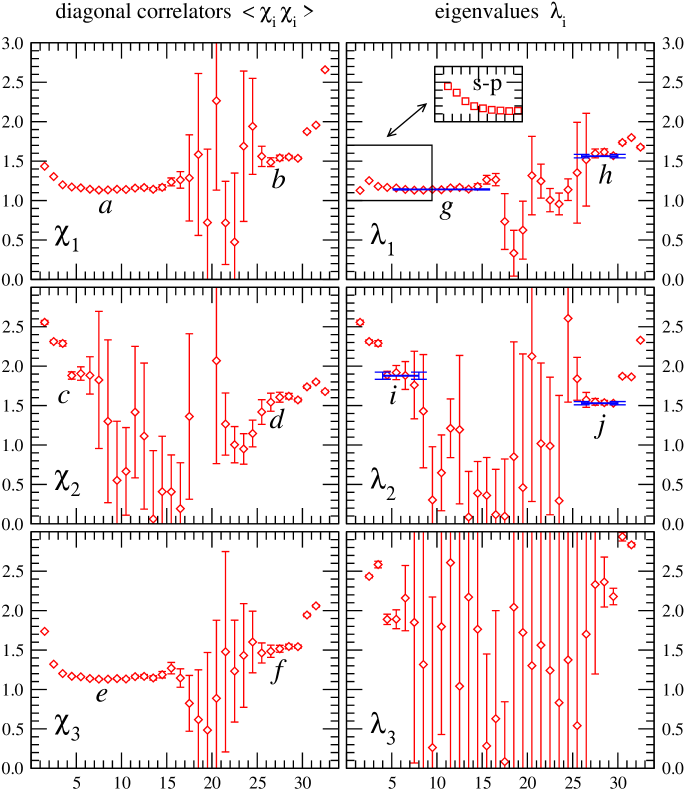
Figure 1: Effective mass plots for the $16^{3}\times 32$ ensemble at $a\,m_{q}=0.10$. The lhs. column shows results from the independent diagonal correlators $\langle\chi_{1}\chi_{1}\rangle$, $\langle\chi_{2}\chi_{2}\rangle$ and $\langle\chi_{3}\chi_{3}\rangle$ (top to bottom) while the rhs. column is for the eigenvalues $\lambda_{i}$ of the correlation matrix. The horizontal bars show our fitting results and range. The characters in the plots label structures which we discuss in the text. The insert in the top right panel demonstrates the effect of turning off the smearing of the sink.

Let us first discuss the independent diagonal correlators $\langle\chi_{i}\chi_{i}\rangle$ shown in the lhs. column. The positive parity states are extracted from the left part ($t<18$) of the plots, while the negative parity states that couple to the same interpolator dominate the right part ($t>18$) of the plots. One clearly sees a good plateau for the interpolators $\chi_{1}$ and $\chi_{3}$ in the interval (5, 15). This plateau corresponds to the ground state nucleon (positions $a$ and $e$). At small Euclidean times one can see contributions from the excited states of positive parity. If an interpolator couples strongly to the nucleon ground state (as it is the case for $\chi_{1}$ and $\chi_{3}$) then the signal from the excited states is only weak and the extraction of the mass for the excited states becomes a complicated task.

The signal obtained with the interpolator $\chi_{2}$ is intriguing. There is no plateau corresponding to the nucleon ground state. This fact has a natural explanation within a quark model and will be discussed below. However, for relatively large quark masses $a\,m_{q}\geq 0.08$ one sees a plateau at smaller distances (3, 7), i.e. position $c$. We remark that for the $a\,m_{q}=0.10$ shown in the figure the quality of this plateau is already very poor, but it is more pronounced at our larger quark masses. The mass corresponding to this plateau is higher than the mass of the negative parity state seen from the same interpolator. Though we do not know the fate of this excited positive parity state at small quark masses, it is unlikely to be the Roper (cf. our discussion in Section VII).

Let us now look at the signals for negative parity states from the diagonal correlators $\langle\chi_{i}\chi_{i}\rangle$. All three of them show plateaus for time intervals (25,30), i.e. positions $b,d,f$. Similar to the plateaus for the excited positive parity state these plateaus are more pronounced for larger quark masses and vanish entirely below $a\,m_{q}=0.06$. It is interesting to note that the plateau in $\langle\chi_{2}\chi_{2}\rangle$ (position $d$) is somewhat higher than the other two plateaus (positions $b,f$). This is consistent with an observation we present below where we will show that at relatively large quark masses the heavier negative parity state $N(1650)$ has a larger $\chi_{2}$ component, while this component is smaller for the lighter $N(1535)$.

The different states which appear in the individual diagonal correlators are separated when analyzing the eigenvalues of the correlation matrix. The corresponding effective mass plots are shown in the rhs. column of Fig. 1. We order the eigenvalues $\lambda_{i}(t)$ with respect to their size, such that for each value of $t$ we have $\lambda_{1}(t)>\lambda_{2}(t)>\lambda_{3}(t)$. The nucleon ground state gives rise to a well pronounced plateau in $\lambda_{1}$ in the time interval $(5,15)$ (position $g$). For the first excited positive parity state there is a hint of a plateau in the range (4,8) (position $i$), but the quality is as poor as for the correlator $\langle\chi_{2}\chi_{2}\rangle$ alone. We remark that there is no sign of the excited states contribution seen in the $\lambda_{1}$ plot at small times. The quality of the plateaus for the two negative parity states (positions $h$ and $j$) is somewhat better. These plateaus become more pronounced for larger quark masses but vanish entirely for $a\,m_{q}<0.06$. As is obvious from the bottom right plot the third eigenvalue $\lambda_{3}$ is highly contaminated with excited states, has large statistical errors, and no structure is visible in the corresponding effective mass plots.

For our variational analysis the number of independent operators should be sufficiently large and was limited to three for practical reasons. However, we also check our results by analyzing also the ($\chi_{1}$, $\chi_{2}$)-subsector. It turns out that the resulting eigenvalues are close to those in Fig. 1. Actually $\chi_{3}$ seems to contribute to the same states as represented by the other two operators and no clear signal to further states is observed. This is further discussed in Sect. VII, but also seen in Fig. 1, where $\lambda_{3}$ shows no additional plateau signal.

In the insert (window) in the upper right plot of Fig. 1 we show the effect of omitting the Jacobi smearing at the sink. All the correlators shown in Figs. 1 and 2 are obtained with both smeared source and sink. The Jacobi smearing is designed to improve the overlap with the ground state and the insert demonstrates clearly, that the contribution of excited states increases when omitting the smearing of the sink. For the point-type sink one now observes a stronger signal from excited states at small time. Note also that since this signal appears in the $\lambda_{1}$ plot, and the $\lambda_{2}$ plot still exhibits a plateau (which originates from the $\chi_{2}$ correlator), we conclude that this signal comes from the $\chi_{1}$ interpolator and the corresponding excited state is not the same as seen with the $\chi_{2}$ interpolator. We have tried to analyze the $\chi_{1}$ correlator with two- and multi-exponential fits in an attempt to extract this positive parity excited state. However, the statistical errors are too large for a reliable extraction and we cannot draw firm conclusions about the ordering relative to the negative parity state. Hence we cannot decide from such a fit about the energy of the lowest positive parity excited state seen with the smeared source and point sink. While we cannot conclude anything concrete whether this signal comes from the Roper resonance or not, the insert shows that optimizing the spatial structure of the nonlocal correlators (in order to possibly separate the signals from the nucleon and the Roper) and introducing more operators is one of the possibilities for further lattice studies of the Roper state.

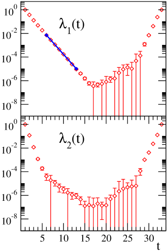
Figure 2: The eigenvalues $\lambda_{1}(t)$ and $\lambda_{2}(t)$ on a logarithmic scale. The data are for $16^{3}\times 32$ at $a\,m_{q}=0.04$). The full line in the $\lambda_{1}$-plot (top) shows the fit for the nucleon mass.

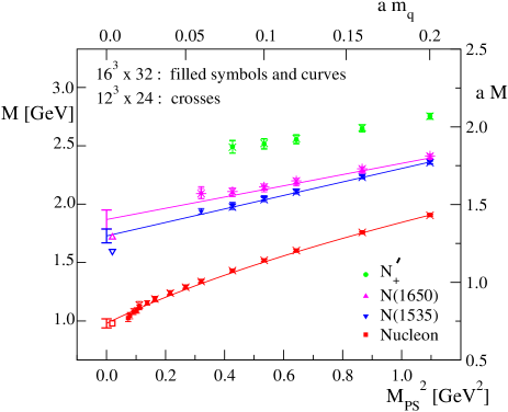
Figure 3: Masses of positive and negative parity states in GeV and in lattice units as a function of the pseudoscalar mass squared in $\textrm{GeV}^{2}$ (quark mass in lattice units on top scale). We show data from $16^{3}\times 32$ lattices as filled symbols and compare them to data from $12^{3}\times 24$ lattices (crosses). The curves represent the chiral extrapolation of the nucleon and the two negative parity states. The open symbols show the experimental values.

Let us finally comment on an interesting structure which we observe both in the $\chi_{2}$ correlator and in $\lambda_{2}$ for small quark masses. In Fig. 2 we illustrate this effect by comparing $\lambda_{1}(t)$ and $\lambda_{2}(t)$ on a logarithmic scale for the $16^{3}\times 32$ ensemble at $a\,m_{q}=0.04$. The top plot shows $\lambda_{1}(t)$ and the full line indicates where we fitted the nucleon mass. The behavior of the second eigenvalue $\lambda_{2}(t)$ (bottom plot) shows a somewhat surprising behavior: It starts off with a large slope but near $t=7$ turns into a nearly linear behavior with a much smaller slope, in particular its absolute value is smaller than the one for the nucleon. If one interprets this as the trace of a physical positive parity particle it would be lighter than the nucleon. As a consequence we cannot interpret this structure as a signal from a physical state, but likely it is related to some quenched artifact. We remark that also the time behavior of the corresponding eigenvector (see Sect. VI) shows a change near $t=7$ indicating that the left half of the $\lambda_{2}(t)$ does not describe a proper physical state.

V Results for the mass spectrum

Table 1: Fit results of fits to $\lambda_{1}$ and $\lambda_{2}$. The nucleon ground state is obtained from smeared–smeared results, whereas the remaining states are from smeared–point calculations. The mass values are in lattice units, the fit interval is denoted by $t$.

$\mathbf{16^{3}\times 32}$, $\mathbf{\bm{\beta_{LW}}=7.90}$					$\mathbf{12^{3}\times 24}$, $\mathbf{\bm{\beta_{LW}}=7.90}$
$a\,m_{\textrm{q}}$	$t$	$a\,M_{N}$	$\chi^{2}_{\textrm{d.o.f.}}$		$a\,m_{\textrm{q}}$	$t$	$a\,M_{N}$	$\chi^{2}_{\textrm{d.o.f.}}$
0.013	$[5,9]$	0.770 (23)	1.31		$[16,22]$
0.014	$[5,10]$	0.786 (20)	1.31
0.016	$[5,11]$	0.811 (19)	1.47
0.018	$[6,12]$	0.826 (16)	1.27
0.02	$[6,12]$	0.839 (15)	1.28		0.02	$[5,9]$	0.853 (23)	1.26
0.025	$[6,12]$	0.868 (14)	1.18
0.03	$[6,13]$	0.892 (13)	1.39		0.03	$[5,10]$	0.893 (17)	0.58
0.04	$[6,13]$	0.935 (11)	1.01		0.04	$[5,11]$	0.931 (14)	0.25
0.05	$[6,14]$	0.972 (09)	0.75		0.05	$[5,12]$	0.969 (12)	0.43
0.06	$[6,14]$	1.008 (08)	0.66		0.06	$[5,12]$	1.005 (11)	0.53
0.08	$[6,14]$	1.077 (07)	0.73		0.08	$[5,12]$	1.075 (09)	0.75
0.10	$[6,15]$	1.141 (06)	1.07		0.10	$[5,12]$	1.142 (08)	0.93
0.12	$[6,15]$	1.204 (05)	1.12		0.12	$[5,12]$	1.205 (07)	1.05
0.16	$[6,15]$	1.321 (05)	1.15		0.16	$[5,13]$	1.321 (07)	1.22
0.20	$[6,16]$	1.433 (04)	1.34		0.20	$[5,13]$	1.431 (06)	1.09
$am_{\textrm{q}}$	$t$	$aM_{N^{\prime}_{+}}$	$\chi^{2}_{\textrm{d.o.f.}}$		$am_{\textrm{q}}$	$t$	$aM_{N^{\prime}_{+}}$	$\chi^{2}_{\textrm{d.o.f.}}$
0.08	$[4,7]$	1.873 (41)	0.15		0.08	$[4,8]$	1.869 (39)	0.04
0.10	$[4,8]$	1.889 (32)	0.17		0.10	$[4,8]$	1.894 (31)	0.96
0.12	$[4,9]$	1.918 (28)	0.26		0.12	$[4,8]$	1.924 (26)	0.94
0.16	$[4,9]$	1.989 (22)	0.70		0.16	$[4,8]$	1.993 (21)	1.12
0.20	$[4,9]$	2.068 (19)	1.46		0.20	$[4,8]$	2.069 (18)	1.66
$am_{\textrm{q}}$	$t$	$aM_{N(1535)}$	$\chi^{2}_{\textrm{d.o.f.}}$		$am_{\textrm{q}}$	$t$	$aM_{N(1535)}$	$\chi^{2}_{\textrm{d.o.f.}}$
0.06	$[27,30]$	1.457 (18)	0.04
0.08	$[26,30]$	1.498 (15)	0.10		0.08	$[19,22]$	1.484 (15)	0.22
0.10	$[26,30]$	1.544 (14)	0.08		0.10	$[18,22]$	1.532 (13)	0.09
0.12	$[26,30]$	1.590 (12)	0.22		0.12	$[17,22]$	1.579 (12)	0.21
0.16	$[25,30]$	1.684 (11)	1.10		0.16	$[17,22]$	1.675 (10)	1.11
0.20	$[25,30]$	1.776 (10)	2.02		0.20	$[16,22]$	1.769 (09)	2.25
$am_{\textrm{q}}$	$t$	$aM_{N(1650)}$	$\chi^{2}_{\textrm{d.o.f.}}$		$am_{\textrm{q}}$	$t$	$aM_{N(1650)}$	$\chi^{2}_{\textrm{d.o.f.}}$
0.06	$[27,30]$	1.577 (38)	0.13		0.06	$[18,22]$	1.570 (33)	1.03
0.08	$[27,30]$	1.578 (26)	0.07		0.08	$[18,22]$	1.584 (23)	0.32
0.10	$[26,30]$	1.604 (21)	0.39		0.10	$[18,22]$	1.613 (19)	0.13
0.12	$[26,30]$	1.638 (18)	0.39		0.12	$[17,22]$	1.652 (16)	0.32
0.16	$[25,30]$	1.716 (15)	0.37		0.16	$[17,22]$	1.730 (14)	0.47
0.20	$[25,30]$	1.800 (13)	0.30		0.20	$[16,22]$	1.813 (12)	0.53

Let us now come to the presentation of the nucleon masses which we extract from our correlators. In Fig. 3 we show the baryon masses in lattice units as a function of the quark mass. Only data points were included where the standards of our fits discussed in Section II could be maintained and where a credible signal in the effective mass plot is seen. They all come from the diagonalization approach using $t_{0}=1$. We did try $t_{0}$ up to 3. The quality of the plateaus does not improve and the results remain invariant. Note that we use Jacobi smeared sources and there we find that these effects are minimal. This behavior changes for more extended sources. All fit results and parameters are listed in Table 1.

The lowest lying set of data corresponds to the ground state in the positive parity sector, i.e. the nucleon. This is followed by two negative parity states which upon simple chiral extrapolation we identify as $N(1535)$ and $N(1650)$. For brevity we use this particle data book nomenclature in the following. Although the two negative parity states are relatively close to each other we clearly separate them with the variational technique discussed above. The fact that the two negative parity states become approximately degenerate towards larger quark masses is well understood in potential models for heavy quarks. Finally, the excited state with positive parity is found on top and we will refer to it as $N_{+}^{\prime}$. While we can identify the nucleon down to rather small quark masses, there is no clear signal (effective mass plateau) for the negative parity states and for the $N_{+}^{\prime}$ at small quark masses. However, below we will show that all states, except for the excited positive parity state $N_{+}^{\prime}$, extrapolate well to their physical masses.

For a study of excited states an analysis of finite volume effects is particularly important. Excited states have more extended wave functions than the ground state and thus suffer more easily from squeezing them into a too small volume. Such a squeezing typically increases the kinetic energy of the constituent quarks and so pushes up the mass of the state. In order to analyze the finite volume effects, in Fig. 3 we compare our numbers for the baryon masses as a function of the bare quark mass $m_{q}$ for $16^{3}\times 32$ and $12^{3}\times 24$ lattices and find little volume dependence.

Our nucleon data easily penetrate the low pion mass region where level crossing of the negative and positive parity states has been claimed in leeetal ; dongetal ; sasaki . However, we find that for the other states the quality of our data depletes with decreasing quark masses and we could not maintain the standards of our fits for $a\,m_{q}<0.06$. We analyzed our data also with other methods (multi-exponential fits, Bayesian priors, maximum entropy method) but did not obtain stable, convincing results for an excited positive parity state $N_{+}^{\prime}$ below quark masses of $a\,m_{q}=0.06$ as well as for the other positive parity excited state extracted form the $\chi_{1}$ correlator. Although leeetal ; dongetal ; sasaki use slightly larger lattices (3.0 fm as opposed to our 2.4 fm) we cannot blame finite size effects for the depletion of the quality of our data, since we obtain essentially unchanged results already on our 1.8 fm lattice.

The masses of the three states nucleon, $N(1535)$ and $N(1650)$ are extrapolated to the chiral limit. For the nucleon this is done by a linear extrapolation of the square of the nucleon mass $(a\,M_{N})^{2}$ as a function of the quark mass $a\,m_{q}$. For the negative parity states we extrapolate linearly the mass as a function of the quark mass. Since the residual quark mass is so small ($a\,m_{res}=-0.0020(5)$) it was neglected in our chiral extrapolation. We used fully correlated fits to take into account the fact that the data for different quark masses were calculated on the same ensemble of configurations and thus are not independent. All three fits have a $\chi^{2}/d.o.f.$ less than 1. The linear extrapolation neglects chiral non-analyticities. We remark that we also experimented with functional forms suggested by quenched chiral perturbation theory LaSh . However, our numerical data are not sufficiently precise for a clear distinction between the simple fits described above and the form from quenched chiral perturbation theory. Thus we decided to stay with the simpler 2-parameter fits.

To set the scale we use either the $\rho$-mass (from bgrlarge ) or give our results as ratios. In Table 2 we list our final numbers for the masses in the chiral limit. We find that the nucleon mass matches its physical value reasonably well and the two negative parity states are about 8 % and 9 % too high. Given the fact that this is a quenched calculation the agreement of our results with experimental data is good. In order to estimate the systematic error from the scale setting we compare the scale from the $\rho$-mass to the scale from the Sommer parameter ($a_{\rho}=0.154(8)$ fm, $a_{r_{0}}=0.148(2)$ fm). The second error given in the dimensionful results in the first line of Table 2 was computed from the difference of the two scales.

Table 2: Comparison of our $16^{3}\times 32$ results in the chiral limit to experimental data. Masses are given in MeV, the ratios are dimensionless numbers.

	$M_{N}$	$M_{N(1535)}$	$M_{N(1650)}$
data	941(38)(28)	1661(57)(65)	1796(78)(70)
exp.	938	1535(20)	1650(30)
		$M_{N(1535)}/M_{N}$	$M_{N(1650)}/M_{N}$
data		1.77(7)	1.91(9)
exp.		1.63(2)	1.75(3)

Like other authors blumetal ; parityminussplita ; parityminussplitb ; leeetal ; dongetal ; sasaki . we also observe a smooth increase of the $N$ – $N(1535)$ splitting towards the chiral limit. At large current quark masses the hadrons may be described as a system with orbital motion in a color-electric confining field and the splitting is due to this orbital excitation. The splitting slowly increases towards the chiral limit implying the increasing importance of another mechanism (spontaneous chiral symmetry breaking) in addition to confinement. This is consistent with the chiral constituent quark model G where an appreciable part of the splitting is related to the flavor-spin interaction between valence quarks.

VI The operator content of physical states

Not only the eigenvalues of the correlation matrix $M$ in Eq. (4) but also the corresponding eigenvectors provide interesting information. In particular the entries of the eigenvectors give the mixing coefficients for the optimal operators $\widetilde{\chi}_{i}$ which have maximal overlap with the physical states in terms of the original basis $\chi_{i}$. Let us be a little bit more explicit. The unnormalized matrix $M_{i,j}(t)$ of Eq. (4) is diagonalized by a unitary matrix $U$ which is built from the eigenvectors $\vec{e}^{\,(i)}$, i.e.

$$U\;M(t)\;U^{\dagger}=\mbox{diag}\Big{(}\lambda_{1}(t),\lambda_{2}(t),\lambda_{3}(t)\Big{)}\;,$$ (10)

with $U^{\dagger}=(\vec{e}^{\,(1)},\vec{e}^{\,(2)},\vec{e}^{\,(3)})$, where $\vec{e}^{\,(i)}$ denotes the $i$-th eigenvector corresponding to the eigenvalue $\lambda_{i}(t)$. Inserting the expression Eq. (10) into Eq.  (4) one finds (repeated indices are summed)

$$\Big{\langle}\Big{(}U_{il}\,\chi_{l}(t)\Big{)}\;P^{\pm}\;\Big{(}U_{jk}\,\chi_{k}(0)\Big{)}^{\dagger}\Big{\rangle} \equiv \langle\widetilde{\chi}_{i}(t)\;P^{\pm}\;\widetilde{\chi}_{j}(0)^{\dagger}\rangle$$ (11)

$$= \delta_{ij}\lambda_{i}(t)\;.$$

Thus the optimal operators $\widetilde{\chi}_{i}$ which have maximal overlap with the physical states are obtained as linear combinations of our original operators $\chi_{i}$,

$$\widetilde{\chi}_{i}=\sum_{j}c^{(i)}_{j}\,\chi_{j}\quad\textrm{with}\quad c^{(i)}_{j}=\vec{e}^{\,(i)\,*}_{j}\;.$$ (12)

Thus the entries of the $i$-th eigenvector $\vec{e}^{\,(i)}$ provide the mixing coefficients for the optimal operator $\widetilde{\chi}_{i}$ coupling to the $i$-th state.

The coefficients $c^{(i)}_{j}$ are not only interesting from a technical point of view for constructing the optimal operator, but also provide interesting insight into the physics of the nucleon system. These physical aspects will be addressed in detail in the next section.

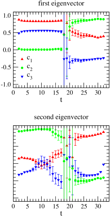
Figure 4: The mixing coefficients $c_{i}$ from the first and second eigenvector as a function of $t$. The data are for $a\,m_{q}=0.12$, $16^{3}\times 32$.

With the normalization chosen for our operators $\chi_{i}$ the coefficients $c_{j}$ are real within error bars, i.e. the imaginary parts are at least two orders of magnitude smaller than the real parts and in the following we only use the real parts . In Fig. 4 we show the coefficients $c_{j}$ determined from the first and second eigenvector which determine the optimal operator for the ground state and the excited state.

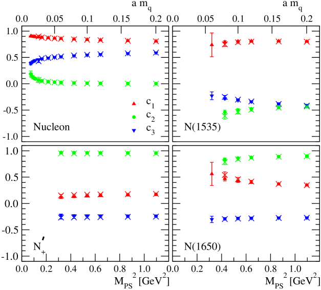
Figure 5: The mixing coefficients $c_{i}$ as a function of the pseudoscalar mass squared (or dimensionless quark mass on top scale). We use large symbols for the $16^{3}\times 32$ data and superimpose the results from $12^{3}\times 24$ with crosses. Note that the $c_{i}$ are amplitudes and only the sum of their squares adds up to 1, i.e.  $|c_{1}|^{2}+|c_{2}|^{2}+|c_{3}|^{2}=1$.

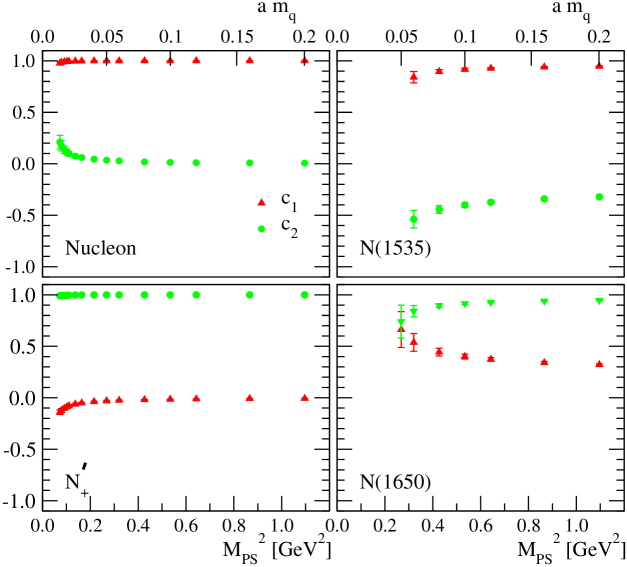
Figure 6: Like the preceding figure, but restricting the space of operators to $\chi_{1}$ and $\chi_{2}$. The sum of the coefficient squares adds up to 1, i.e. $|c_{1}|^{2}+|c_{2}|^{2}=1$.

Strictly speaking the matrix $U$ which is used in Eq. (10) to diagonalize the correlation matrix $M(t)$ is time dependent. However, for a proper physical state one expects that the coefficients are independent of $t$ within the time interval that corresponds to the given physical state. The time independence of the coefficients is well pronounced for the nucleon ($t=3\,\ldots\,17$ in the top plot) and also for the two negative parity states ($t=22\,\ldots\,30$). The regions of constant $c_{j}$ agree nicely with the regions where we find plateaus in the effective masses. Only in the crossing region near $t=19$ and close to $t=1$ for the positive parity states, respectively $t=32$ for the negative parity states, where higher excited states still contribute we find strong deviation from a constant behavior. Only the excited positive parity state which is seen in the second eigenvector effective mass plot of Fig.1 does not show long regions with $t$-independent coefficients. It seems that this channel is for small $t$ dominated by an excited state between $t=2$ and $t=7$ and then changes to a lower-lying state with different values for the $c_{i}$ visible until $t=17$. This additional mixing is clearly reflected in the problems which we encountered when trying to fit the mass of the state $N_{+}^{\prime}$. The corresponding low-lying artifact was discussed in Section 4 and the corresponding structure in the correlator was shown in Fig. 2.

An interesting question is how the coefficients depend on the quark mass or pion mass. In order to address this question we take for each state at each value of the quark mass the values of the corresponding coefficients in the center of the effective mass plateau. In particular we chose $t=8$ for the coefficients of the nucleon, $t=28$ for the two negative parity states (this value changes to $t=20$ on the $12^{3}\times 24$ lattice) and $t=5$ for the state $N_{+}^{\prime}$. In Fig. 5 we plot the coefficients as a function of the pseudoscalar mass (the data for $M_{PS}$ were taken from bgrlarge ) and compare the results from $16^{3}\times 32$ (symbols) to $12^{3}\times 24$ (thin crosses) in order to check for finite size effects.

The absence of finite size effects which was already seen for the masses is now also supported by our findings for the coefficients. The results from $12^{3}\times 24$ (crosses) agree with the data from $16^{3}\times 32$ within error bars. It is obvious that the coefficients show a non-trivial mass dependence. The coefficients necessary for the construction of the optimal operators $\widetilde{\chi_{i}}$ which couple to the $i$-th state can be read of directly from the figure. We remark that the optimal operators $\widetilde{\chi_{i}}$ are a powerful tool which can be used to study properties of excited states other than just their mass such as e.g. matrix elements.

VII Physical interpretation of the mixing coefficients

As mentioned, the time component of operator $\chi_{3}$ couples to the spin $1/2$ state. In order to check its influence we also study the ($\chi_{1}$, $\chi_{2}$)-subsector alone. Fig. 6 gives the resulting mixing coefficients analogous to Fig. 5. We find, that $\chi_{1}$ and $\chi_{2}$ behave similar in both cases and that $\chi_{3}$ plays a subordinate role. Due to the different definition (e.g. our states are orthogonal and normalized) it is difficult to compare the numbers of Fig. 6 with the results of parityminussplita . In both cases, as in blumetal , the nucleon is overwhelmingly due to $\chi_{1}$ while $N^{\prime}_{+}$ is mostly due to $\chi_{2}$.

First, we would like to give a simple explanation, based on a quark model picture, why the interpolator $\chi_{2}$ couples only weakly to the nucleon. According to the quark model the nucleon belongs to the 56 representation of $SU(6)$. Its flavor-spin wave function is completely symmetric with respect to permutation of two constituent quarks. Since the color wave function is completely antisymmetric, the Pauli principle requires that the wave function must by symmetric with respect to permutation of the spatial coordinates of any two constituent quarks. Hence the parity of any diquark subsystem is positive. Consequently the pure $SU(6)$ symmetric nucleon wave function does not contain any pseudoscalar or vector diquark subsystems and the nucleon cannot couple to the interpolator $\chi_{2}$. This argument is exact in the large $N_{c}$ limit.

The other question is why the nucleon couples to $\chi_{1}$ much stronger than to $\chi_{3}$ in spite of both having similar diquark content. The answer is that the interpolators belong to different chiral representations (as discussed in Sect. 3). If chiral symmetry was not broken then each hadronic state would couple to the interpolator with concrete transformation properties under $SU(2)_{L}\times SU(2)_{R}$. Chiral symmetry breaking implies that the nucleon does not belong to any specific representation and couples to $\chi_{1},\chi_{3}$ and weakly also to $\chi_{2}$, all of them belonging to distinct representations. The stronger coupling to $\chi_{1}$ indicates that the corresponding representation $(0,1/2)+(1/2,0)$ dominates the nucleon wave function.

The $SU(6)$ symmetry is broken by the residual spin-spin and other interactions, which are corrections of ${\cal O}(1/N_{c})$. The weight of the components that contain pseudoscalar or vector diquark subsystems is very small (e.g. for a chiral quark model cf. Ref. GV ). This explains why the component $c_{2}$ is small in the panel for the nucleon in Fig. 5 and why one does not see the nucleon from the interpolator $\chi_{2}$. While we do observe some coupling of the nucleon to the interpolator $\chi_{3}$ the corresponding amplitude $c_{3}$ in the upper lhs. plot is small. We stress that the $c_{i}$ are amplitudes, i.e. their squares are probabilities adding up to 1.

Within the quark model the Roper state belongs to the other 56 representation of $SU(6)$. The Roper is a radial excitation of the spatial part of the nucleon wave function. Hence all the arguments given above for the nucleon apply also to the Roper. However, the coefficients plot for the $N^{\prime}_{+}$ (lower lhs. plot in Fig. 5) shows a large component $c_{2}$ and assuming the quark model picture one concludes that the $N^{\prime}_{+}$ state seen with either the diagonal $\chi_{2}$-correlator or with the eigenvalue $\lambda_{2}$ is not the Roper state. A possible candidate for the $N^{\prime}_{+}$ state could be some higher-lying positive parity state as e.g. the $N(1710)$, which does contain a large pseudoscalar diquark component in its wave function.

Another important issue which we would like to discuss is the pronounced quark mass dependence of the mixing coefficients $c_{i}$ for the $N(1535)$ and $N(1650)$ states, shown in the two rhs. plots of Fig. 5. One clearly sees that while at large quark masses the $N(1535)$ is dominated by $\chi_{1}$ and the $N(1650)$ by $\chi_{2}$, the situation becomes different towards the chiral limit. This feature persists also when studied just a subset of operators as in Fig. 6. Upon extrapolation to the chiral limit the $N(1535)$ couples optimally (up to some uncertainty) to $(\chi_{1}-\chi_{2})$, while $N(1650)$ couples to $(\chi_{1}+\chi_{2})$ and the contribution of $\chi_{3}$ is suppressed for both negative parity states. The very fact that the mixing towards the chiral limit is quite different from that in the heavy quark region implies that the physics of these resonances (and in particular of their wave functions) is strongly influenced by chiral symmetry and its spontaneous breaking. It is interesting to try to connect this behavior to the quark model. Both $N(1535)$ and $N(1650)$ belong to the negative parity $L=1$ 70-plet of $SU(6)$. Each member of this multiplet contains in its wave function both scalar and pseudoscalar diquark components. The mixing of these two different components is provided by tensor forces.

A proper mixing of two independent components does explain, in particular, peculiarities of the $N^{*}\rightarrow N\eta$ decays. One can construct a linear combination such that the $N\eta$ decay of the $N(1650)$ gets strongly suppressed, while the decay of the $N(1535)$ gets enhanced. There are two possible origins of a tensor force providing the necessary mixing: The tensor force which is supplied by perturbative gluon exchange and which does not contain flavor dependence in its operator structure ISGUR and the tensor force mediated by the Goldstone field and related to spontaneous chiral symmetry breaking G ; TENSOR . If the mixing was due to perturbative gluon exchange one would not expect that the mixing would depend on the current quark mass. However, a tensor force that originates from chiral symmetry breaking appears only towards the chiral limit. Our lattice results, shown in Figs. 5 and 6, clearly support the latter possibility, though these results cannot shed any light on the specific microscopical origin of the tensor force. This result is also consistent with the recent phenomenological COLL and large $N_{c}$ 1/N analyses of the mixing of the negative parity baryons: Both studies suggest that a proper mixing is supplied by the flavor-dependent tensor force.

Finally, our results allow to explain the smallness of the $\pi NN(1535)$ and $\pi NN(1650)$ coupling constants as compared to the large $\pi NN$ coupling. It has been shown in Ref. OKA that if both the nucleon and $N(1535)$ (or $N(1650)$) are created from the vacuum only by the $\chi_{1}$ and $\chi_{2}$ interpolators, irrespective of their mixing, then the chiral symmetry properties of these interpolators imply that the $\pi NN(1535)$ and $\pi NN(1650)$ couplings must vanish. In the present work we find that the coupling of all these baryons to the interpolator $\chi_{3}$, which belongs to another representation of the chiral group, is much smaller than the coupling to $\chi_{1}$ or $\chi_{2}$. This qualitatively explains the smallness of the $\pi NN(1535)$ and $\pi NN(1650)$ coupling constants.

VIII Conclusions

Let us summarize our main findings. We use three different interpolating fields and study how these fields couple to the nucleon and its excited states of both parities. We clearly identify distinct negative parity excited states $N(1535)$ and $N(1650)$ and show that the mixing of different interpolators which create these baryons from the vacuum, is obviously quark mass dependent. The mixing towards the chiral limit is qualitatively different from the mixing in the heavy quark region. This implies that the physics of these states is strongly related to chiral symmetry of QCD. A very specific mixing which is observed towards the chiral limit can be a basis for the explanation of $N^{*}\rightarrow N\eta$ and $N^{*}\rightarrow N\pi$ decays of these baryons.

In a quark model picture we are able to understand peculiarities of the coupling of different interpolators to the nucleon and its excited states.

We clearly see an excited state of positive parity at relatively large quark masses from the interpolator $\chi_{2}$. Although we cannot reliably trace this state towards the chiral limit we argue that it lies too high for an identification as the Roper resonance and may correspond to the $N(1710)$ state.

While we do observe some contribution of positive parity excited state(s) to the $\chi_{1}$ interpolator at small times, the signal is rather weak and using traditional methods, such as effective mass plots or one (two, many)-exponential fits of the correlator, do not allow us to conclude whether this signal comes from the Roper state or from some higher lying states. It would be an important task to optimize source and sink in order to improve the signal from the Roper resonance.

In dongetal the subtraction of a parametrization of possible quenched artifacts ($\eta^{\prime}N$) — giving rise to negative values of the correlation function for central $t$-values — was crucial for the identification of a Roper signal. We also observe such negative values but postpone an analysis to future studies with better statistics.

An interesting challenge for further lattice studies is the empirically observed approximate parity doubling of nucleons above 1.7 GeV region (and similar in delta spectrum). It has been suggested that this doubling may reflect a smooth effective chiral symmetry restoration in the upper part of hadron spectra CG . Still, there remains the possibility that this doubling is accidental. Lattice methods can help to clarify this interesting issue.

- (1) C. Davies, The heavy hadron spectrum, in: Computing Particle Properties, H. Gausterer, C. B. Lang (Eds.), Lecture Notes in Physics, V. 512, Springer, 1998.
- (2) R. Dashen and A. Manohar, Phys. Lett. B 315, 425 (1993); E. Jenkins, Ann. Rev. Nucl. Part. Sci. 48, 81 (1998).
- (3) L. Ya. Glozman and D. O. Riska, Phys. Rep. 268, 263(1996); L. Ya. Glozman et al. Phys. Rev. D 58, 094030 (1998); L. Ya. Glozman, Plenary talk at PANIC 99, Nucl. Phys. A 663, 103 (2000).
- (4) F. X. Lee and D. B. Leinweber, Nucl. Phys. (Proc. Suppl.) 73, 258 (1999); S. Sasaki et al., Nucl. Phys. (Proc. Suppl.) 119, 302 (2003); D. G. Richards et al. [LHPC Collaboration], Nucl. Phys. Proc. Suppl. 109, 89 (2002); D. G. Richards, Nucl. Phys. (Proc. Suppl.) 94, 264 (2001).
- (5) S. Sasaki, T. Blum and S. Ohta, Phys. Rev. D 65, 074503 (2002).
- (6) W. Melnitchouk et al., Phys. Rev. D 67, 114506 (2003);
- (7) R. G. Edwards, U. Heller and D. Richards, Nucl. Phys. (Proc. Suppl.) 119, 305 (2003); F. X. Lee [Lattice hadron physics collaboration], Nucl. Phys. Proc. Suppl. 94, 251 (2001).
- (8) F. X. Lee et al., Nucl. Phys. (Proc. Suppl.) 119, 296 (2003).
- (9) S. J. Dong et al., arXiv:hep-ph/0306199.
- (10) S. Sasaki, Prog. Theor. Phys. Suppl. 151, 143 (2003).
- (11) C. Michael, Nucl. Phys. B 259, 58 (1985); M. Lüscher and U. Wolff, Nucl. Phys. B 339, 222 (1990).
- (12) C. Gattringer, Phys. Rev. D 63 (2001) 114501; C. Gattringer, I. Hip, C. B. Lang, Nucl. Phys. B 597, 451 (2001).
- (13) M. Lüscher and P. Weisz, Commun. Math. Phys. 97, 59 (1985); Err.: 98, 433 (1985); G. Curci, P. Menotti and G. Paffuti, Phys. Lett. B 130, 205 (1983), Err.: B 135, 516 (1984).
- (14) C. Gattringer, R. Hoffmann and S. Schaefer, Phys. Rev. D 65, 094503 (2002).
- (15) C. Gattringer et al. [Bern-Graz-Regensburg Collaboration], Nucl. Phys. B 677, 3 (2004).
- (16) A. Hasenfratz and F. Knechtli, Phys. Rev. D 64, 034504 (2001).
- (17) P.H. Ginsparg and K.G. Wilson, Phys. Rev. D 25, 2649 (1982).
- (18) C. Gattringer, Nucl. Phys. B (Proc. Suppl.) 119, 122 (2003); C. Gattringer et al. [Bern-Graz-Regensburg Collaboration], Nucl. Phys. B (Proc. Suppl.) 119, 796 (2003); V.M. Braun et al. Phys. Rev. D 68, 054501 (2003).
- (19) C. Best et al., Phys. Rev. D 56, 2743 (1997).
- (20) B. Jegerlehner, hep-lat/9612914 (1996).
- (21) C. Gattringer and C. B. Lang, Nucl. Phys. B 391, 463 (1993).
- (22) B.L. Ioffe, Nucl. Phys. B 188, 317 (1981); Err.: B 191, 591 (1981); Y. Chung et al. , Nucl. Phys. B 197, 55 (1982).
- (23) T.D. Cohen and L. Ya. Glozman, Phys. Rev. D 65, 016006 (2002); Int. J. Mod. Phys. A 17, 1327 (2002); L. Ya. Glozman, Phys. Lett. B 541, 115 (2002).
- (24) J. N. Labrenz and S. R. Sharpe, Phys. Rev. D 54 (1996) 4595.
- (25) L. Ya. Glozman and K. Varga, Phys. Rev. D 61, 074008 (2000).
- (26) A. DeRujula, H. Georgi and S.L. Glashow, Phys. Rev. D 12, 12 (1975); N. Isgur and G. Karl, Phys. Rev. D 18, 4187 (1978); N. Isgur, Phys. Rev. D 62, 054026 (2000).
- (27) D.O. Riska and G.E. Brown, Nucl. Phys. A 653, 251 (1999); L.Ya. Glozman, Surv. High Energy Phys. 14, 109 (1999); R.F. Wagenbrunn et al., Nucl. Phys. A 663, 703 (2000); Jun He and Yu.-B. Dong, Nucl. Phys. A 725, 201 (2003)
- (28) H. Collins and H. Georgi, Phys. Rev. D 59, 094010 (1999).
- (29) C.E. Carlson et al., Phys. Rev. D 59, 114008 (1999); C.L. Schat, J.L. Goity and N.N. Scoccola, Phys. Rev. Lett. 88, 102002 (2002); D. Pirjol and C. Schat, Phys. Rev. D 67, 096009 (2003).
- (30) D. Jido, M. Oka and A. Hosaka, Phys. Rev. Lett. 80, 448 (1998).
- (31) T.D. Cohen and X. Ji, Phys. Rev. D 55, 6870 (1997).