Abstract

We suggest a simple analytical description of the S-wave isoscalar $\pi\pi$ amplitude, which corresponds to a joint dressing of the bare resonance and background contributions. The amplitude describes well the experimental data on the $\delta^{0}_{0}$ phase shift in the energy region below 900 MeV and has two poles in the $Re\ s>\ 0$ half-plane. Besides the well-known pole of $\sigma(600)$-meson with $Re\ s\sim m_{\pi}^{2}$, there exists a more distant pole with $Re\ s\sim 0.6\ GeV^{2}$. Our analysis indicates for the dynamical origin of the $\sigma(600)$ pole, while the second pole should be associated with lowest $q\bar{q}$ state.

1 Introduction

The properties of the lightest scalar meson $\sigma(600)$ are very important for interpretation of a scalar family and details of the chiral symmetry breaking. Appearance of a new experimental information and the theory development in the low energy region generated an extensive discussion on this issue (see [1, 2, 3, 4, 5] and references therein). As for existence of $\sigma(600)$, now it is a commonly accepted fact and this resonance is included back into Particle Data Group’s tables.

There is a long story concerning the resonance interpretation of the S-wave amplitude $\pi\pi\to\pi\pi$ with isospin I=0. One of the key moments of this story was a realization (see e.g. [6, 7, 8]) that apart of the resonance $\sigma(600)$ term there is an essential background contribution in this energy region. However there is no evident recipe to divide the $\pi\pi$ amplitude into the resonance and background terms. The simplest and widely used method is ”adding in phase shift” of the resonance an background contributions (IA method in terminology of [7, 8]):

$$\delta^{0}_{0}=\delta^{R}+\delta^{B}.$$ (1)

The amplitude $\pi\pi\to\pi\pi$ in this case is:

$$f^{0}_{0}(s) = \frac{e^{2i\delta^{0}_{0}}-1}{2i\rho}=\frac{e^{2i\delta^{B}}-1}{2i\rho}+e^{2i\delta^{B}}\cdot\frac{e^{2i\delta^{R}}-1}{2i\rho}=$$ (2)

$$= \frac{e^{2i\delta^{B}}-1}{2i\rho}+e^{2i\delta^{B}}\cdot f^{Res}(s).$$

The anzats (1) may be derived from summation of the loop contributions with some extra conditions [6]. To obtain the resonance parameters from the experimental data one needs an additional assumption about the form of the background contribution $\delta^{B}$. The best way for a broad resonance is to determine its mass and the width from the pole position in the complex energy plane. However only the resonance contribution $f^{Res}(s)$ of the entire amplitude (2) can be continued into the complex energy plane. Thus it is possibly to study the pole position but not the pole residue.

Other methods to describe the $\delta^{0}_{0}$ phase shift, different from (1), either have the so evident defects, or are much more complicated with many free parameters.

In this paper we suggest a very simple analytical parameterization for $\pi\pi$ amplitude which allows us to continue it to the second Riemann sheet. The amplitude contains (in spirit of the linear $\sigma$-model) two bare objects: the resonance and the background. The main idea is that a joint unitarization of two objects should be described correctly by the field theory methods. As concerning the form of a background contribution at the tree level, it can be modelled by a maximally simple method.

There are different ways to construct such analytical amplitude. We found the suitable one the formalism of the unitary mixing, the obtained amplitude is analytical and unitary automatically. Such construction is rather flexible which allows us to investigate some different physical situations.

Note that from other side the bare pole located at $s<\ 0$ may be considered as some effective cross exchange and its value $m_{2}^{2}\sim-m_{\rho}^{2}$, obtained from a fit, confirms this interpretation. As compared with standard N/D method our amplitude with two bare objects automatically has a zero, which is necessary to describe the S-wave low energy data.

2 Formalism of the unitary mixing

If there exist n bare states with the same quantum numbers then the dressing of their propagators should account also the mutual transitions between them. The process of joint dressing is described in this case by the system of Dyson-Schwinger equations:

$$\Pi_{ij}(s)=\pi_{ij}(s)-\Pi_{ik}(s)J_{kl}(s)\pi_{lj}(s),\ \ \ \ \ \ \ \ \ i,j=1...n.$$ (3)

Here $\pi_{ij}$ and $\Pi_{ij}$ are bare and dressed propagators respectively, $J_{ij}$ are the self-energy contributions.

Let us consider mixing of two resonances (n=2) with one open intermediate state. In this case the solutions of (3) are:

$$\Pi_{11}=\frac{D_{2}(s)}{D(s)},\ \ \ \Pi_{12}=\frac{J_{12}(s)}{D(s)},\ \ \ \Pi_{22}=\frac{D_{1}(s)}{D(s)}.$$ (4)

Here

$$D(s) = D_{1}D_{2}-(J_{12}(s))^{2},$$

$$D_{1} = m_{1}^{2}-s-J_{11}(s),\ \ \ \ \ D_{2}=m_{2}^{2}-s-J_{22}(s).$$ (5)

In the case of scalar resonances interacting with pion pair, the loops are of the form:

$$J_{11}(s)=g_{1}^{2}J(s),\ \ \ J_{22}(s)=g_{2}^{2}J(s),\ \ \ J_{12}(s)=g_{1}g_{2}J(s).$$ (6)

$$J(s)=\frac{s-a}{\pi}\int_{4m_{\pi}^{2}}^{\infty}\ \frac{ds^{\prime}}{(s^{\prime}-a)(s^{\prime}-s)}\ \rho(s^{\prime}),\ \ \ \ \ \ \rho(s)=\sqrt{\frac{s-4m_{\pi}^{2}}{s}},$$ (7)

where $0<a<4m_{\pi}^{2}$ is the subtraction point, $g_{i}$ are the coupling constants.

The $\pi\pi$ amplitude:

$$f=g_{1}^{2}\Pi_{11}(s)+g_{2}^{2}\Pi_{22}(s)+2g_{1}g_{2}\Pi_{12}(s)=\frac{N(s)}{D(s)},$$ (8)

where

$$D(s) = (m_{1}^{2}-s)(m_{2}^{2}-s)-J(s)N(s),$$

$$N(s) = g_{1}^{2}(m_{2}^{2}-s)+g_{2}^{2}(m_{1}^{2}-s).$$ (9)

It is evident that (8) satisfies the elastic unitary condition

$$Im\ f=\rho|f|^{2}.$$ (10)

The above equations can be applied not only for the case of two resonances but also for the ”resonance+background” situation, when one of the bare poles is located at $s<0$. Just right this situation arises for the S-wave I=0 $\pi\pi\to\pi\pi$ amplitude. One can see from (12) that our amplitude is zero at the point:

$$s_{0}^{0}=(g_{1}^{2}m_{2}^{2}+g_{2}^{2}m_{1}^{2})/(g_{1}^{2}+g_{2}^{2}),$$ (11)

which should be $s_{0}^{0}\sim m_{\pi}^{2}$ to reproduce the Adler zero. So we have $m_{2}^{2}\ <\ 0$ .

Let $m_{2}^{2}\ <\ 0$ be the bare zero of function D(s), which stays at the left of real axis after dressing. Then it is convenient to subtract the loop at this point:

$$D(s)=(m_{1}^{2}-s)(m_{2}^{2}-s)-(J(s)-J(m_{2}^{2}))\left[g_{1}^{2}(m_{2}^{2}-s)+g_{2}^{2}(m_{1}^{2}-s)\right].$$ (12)

Below we shall use the amplitude (8), (12) for description of the experimental data. Here $m_{1}^{2},g_{1}^{2},m_{2}^{2},g_{2}^{2}$ are free parameters. The background contribution at the tree level may be modelled by the pole or constant. It is sufficient for successful description of the experimental data as it is seen below.

3 Analysis of $\pi\pi$ data in region of $m_{\pi\pi}<$ 900 MeV

In the nearthreshold region we use the new data from $K_{l4}$ decay [10], which may be seen at Fig. 1 in comparison with 1977 year data [11]. We do not take into account the old data [11] as it has no practical effect on the fit. The measured value in $K_{l4}$ decay is the phase shift difference $\delta_{0}^{0}-\delta_{1}^{1}$ thus we need an additional information on the P-wave. We use for this purpose the approximation of solution of the Roy equations from Ref.[12]. Fortunately, the $\delta_{1}^{1}$ contribution is only about $1.5^{\circ}$ at the end of the interval due to the P-wave threshold behavior, thus the uncertainty in $\delta_{1}^{1}$ is negligible.

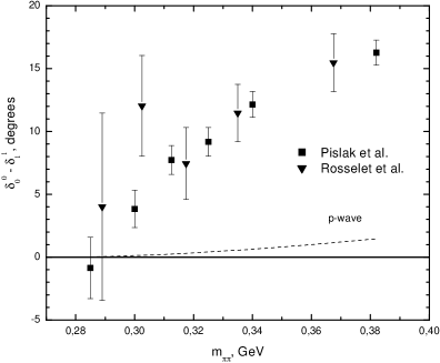
Figure 1: Phase shift difference $\delta_{0}^{0}-\delta_{1}^{1}$ from experiment on $K_{l4}$ decay.

Our main purpose is the $\sigma(600)$ resonance thus we restrict ourselves by the energy region $m_{\pi\pi}<0.9$ GeV. It allows us to use the one-channel approach and not to take into account the $f_{0}(980)$ effect. In this region there exist different experiments and different analyses of S-wave phase shifts, see recent reviews [13, 14].

Below we use only classical partial analyses of Protopopescu et al. [16] from $\pi^{+}p\to\pi^{+}\pi^{-}\Delta^{++}$ reaction and Estabrooks and Martin one of CERN experiment [15] on $\pi^{-}p\to\pi^{+}\pi^{-}n$ (let us call their two solutions for $\delta_{0}^{0}$ phase shift as EM I and EM II). Below we consider the mentioned experimental data on the $\delta_{0}^{0}$ phase shift and find very similar conclusions. As an example we focus in more details on the the EM II solution.

Fig. 2 displays the results of joint fitting of $K_{l4}$ data ($m_{\pi\pi}<0.4$ GeV) and EM II data ($0.51<m_{\pi\pi}<0.9$ GeV). One can see that our amplitude (12) describes well these data.

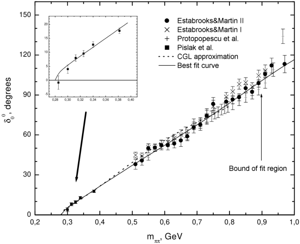
Figure 2: Results of the fit of the $\pi\pi$ phase shift by the amplitude (12). Solid curve is the best fit to the data of $K_{l4}$ decay and EM II its parameters can be seen in the first column of Table 1.

Best fit parameters are:

$$m_{1}^{2} = 0.659\pm 0.041\ GeV^{2},\ \ \ \ \ g_{1}^{2}=0.435\pm 0.036\ GeV^{2},$$

$$m_{2}^{2} = -0.230\pm 0.114\ GeV^{2},\ \ \ g_{2}^{2}=0.177\pm 0.067\ GeV^{2},$$

$$\chi^{2}/DOF = 17.7/21.$$ (13)

Let us consider the zeros of function D(s) at the second Riemann sheet. The procedure of analytical continuation is described in Appendix B. The Fig. 3 shows the zeros location in the complex s plane corresponding to the best fit parameters (13). Let us stress that we find two zeros in the $Re\ s>0$ half-plane.

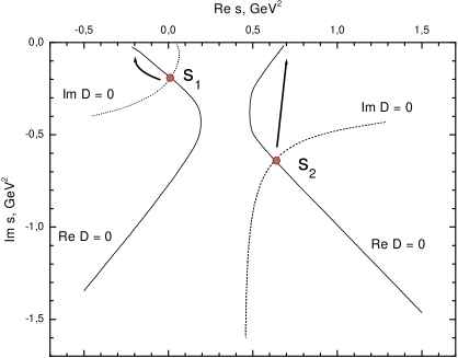
Figure 3: Poles of the amplitude $\pi\pi\to\pi\pi$ with J=I=0 on the second Riemann sheet at parameters (13). Arrows indicate the direction of the poles movement when the interaction is turned off.

The Table 1 represents results of the fit of the different low energy data by our amplitude (12). All data sets lead to the solutions with two poles: close and distant .

$K_{l4}$+EM II	$K_{l4}$+EM I	$K_{l4}$+Protopopescu	CGL [12]
$E<0.9$ GeV	$E<0.9$ GeV	$E<0.9$ GeV	$E<0.8$ GeV
$m_{1}^{2}=0.659\pm 0.041$	$m_{1}^{2}=0.586\pm 0.025$	$m_{1}^{2}=0.794\pm 0.114$	$m_{1}^{2}=0.845$
$g_{1}^{2}=0.435\pm 0.036$	$g_{1}^{2}=0.382\pm 0.020$	$g_{1}^{2}=0.598\pm 0.151$	$g_{1}^{2}=0.779$
$m_{2}^{2}=-0.230\pm 0.114$	$m_{2}^{2}=-0.113\pm 0.053$	$m_{2}^{2}=-0.580\pm 0.405$	$m_{2}^{2}=-0.573$
$g_{2}^{2}=0.177\pm 0.067$	$g_{2}^{2}=0.116\pm 0.030$	$g_{2}^{2}=0.422\pm 0.331$	$g_{2}^{2}=0.548$
$\chi^{2}/DOF=17.7/21$	$\chi^{2}/DOF=22.6/21$	$\chi^{2}/DOF=5.3/19$	$\chi^{2}/DOF=0$
Poles:	Poles:	Poles:	Poles:
$s_{1}=0.015+i\ 0.192$	$s_{1}=0.045+i\ 0.132$	$s_{1}=0.055+i\ 0.339$	$s_{1}=0.104+i\ 0.250$
$s_{2}=0.633+i\ 0.630$	$s_{2}=0.632+i\ 0.533$	$s_{2}=0.484+i\ 1.020$	$s_{2}=0.659+i\ 1.620$

Table 1: Results of the fit of the different sets of experimental data by our amplitude. $m_{i}^{2}$, $g_{i}^{2}$, $s_{i}$ are in units of $GeV^{2}$. In the last column our parameterization is compared to approximation of the phase shift from Ref. [12] (Solution [17] of the Roy equations with use of scattering lengths from the two-loop chiral perturbation theory calculations.). Our phase shift practically coincides with CGL approximation in this energy region.

In Fig.5 we compare phase shifts corresponding to different variants of Table 1.

Figure 4: Phase shifts corresponding to different sets of parameters shown in Table 1.

Figure 5: Data fit at fixed value of the left pole $m_{2}^{2}$.

We can see that our simple model (12) corresponding to joint unitarization of two bare objects: one pole at $s<0$ and another pole at $s>0$ describes successfully the $\pi\pi$ phase shift $\delta_{0}^{0}$ in the energy region below 900 MeV. We find two poles in the complex s plane: one close to the origin with $Re\ s\sim m_{\pi}^{2}$ and the second one with $Re\ s\sim 0.6\ GeV^{2}$. However the behavior of the poles when interaction is turned off $g_{i}^{2}\to 0$ is rather unexpected (see Fig. 3): the close pole traditionally identified with $\sigma(600)$ meson moves to the negative s region. While the second pole $s_{2}$ (most of previous analyses did not observe it) tends to the real axis above the threshold.

As an alternative we can investigate the case when the background has not bare pole. It corresponds to the joint dressing in the system ”$\sigma$-pole + constant”. For this purpose it is sufficient to put the value $m_{2}^{2}$ negative and large in our amplitude (12).

In Fig. 5 there are shown the results of data fit with different $m_{2}^{2}$ values. One can see that the experimental data prefer rather close left pole $|m_{2}^{2}|<0.6\ GeV^{2}$.

Fig. 6 illustrates the pole positions in the complex plane at value $m_{2}^{2}=-1\ GeV^{2}$ and their behavior when interaction is turned off. We observe that the behavior of poles has been changed as compared with $m_{2}^{2}>-0.5\ GeV^{2}$ case.

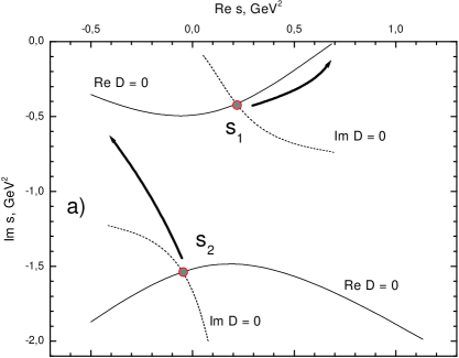
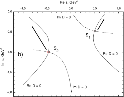
Figure 6: a) Poles positions in the complex s plane at $m_{2}^{2}=-1\ GeV^{2}$ (fit of the data $K_{l4}$+EM II) and their movement at $g_{i}\to 0$.
b) Illustration of the poles movement. As compared with a) we slightly reduced the coupling constants $g_{i}^{2}\to 0.75g_{i}^{2}$ with fixed other parameters.

4 Discussion

We found that the $\pi\pi$ phase shift $\delta_{0}^{0}$ is well described by a simple analytical amplitude (12) in the energy region from the threshold up to 900 MeV. Our amplitude corresponds to a joint dressing of two bare objects: resonance and background contributions. Background can be modelled either by a pole with $Re\ s<0$ or by constant. As a next step one could investigate the more complicated background model: left pole + constant (just as in the linear $\sigma$-model). However since our simple amplitude (12) provides a good description of the experimental data we suppose that inclusion of new degrees of freedom has no meaning.

After the fit of the experimental data we found the presence of two complex poles at the second Riemann sheet: one close to the origin with $Re\ s_{1}\sim m_{\pi}^{2}$ and the second one with $Re\ s_{2}\sim 0.5-0.6\ GeV^{2}$. The close pole was seen in most of the previous analyses of $\pi\pi$ scattering (its position is defined mainly by Adler zero) and it was associated with the lightest scalar meson $\sigma(600)$. Note that we approximated the background term at the tree level by some pole, physically it corresponds to the cross-exchange by $\rho$- or $\sigma$-meson. The existing experimental data certainly prefer the pole form of background as compared with constant.

As for behavior of the poles in the limit of $g_{i}\to 0$ we observe that only the distant pole goes to the real axis at positive s (see Fig. 3). This fact holds true for all variants indicated in Table 1. More detailed investigation shows that such a behavior changes with $m_{2}^{2}$ value as it is schematically illustrated in Fig. 7. The experimental data on $\pi\pi$ scattering with energy below 900 MeV prefer the variant a) while the variant b) with $m_{2}^{2}\sim-1\ GeV^{2}$ also can not be excluded (see Fig. 5). For example, the found $\chi^{2}$ values are $\chi^{2}/DOF=17.7/22$ for a) and $\chi^{2}/DOF=22.6/22$ for b) in one of variants of fit.

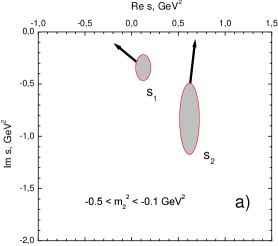
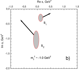
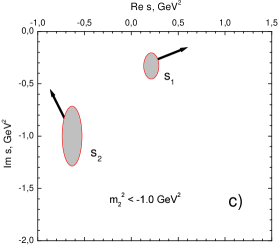
Figure 7: Poles positions in the complex s plane and their movement at $g_{i}\to 0$ is managed by $m_{2}^{2}$ value. The variant a) is preferable by quality of the data description but b) also has an acceptable value of $\chi^{2}$.

In view of discussion [18, 19, 20, 21, 5] whether the $\sigma(600)$ the intrinsic state or it is dynamically generated, our results should be interpreted as an indication for a dynamical nature of the $\sigma(600)$. In this case the second pole should be associated with intrinsic $q\bar{q}$ state having regard to above remarks.

We suppose that the most interesting question is the meaning of the second pole $s_{2}$. It was seen only in a few previous analysis, e.g. in [2], where it was considered as an artefact since it was located out of the considered energy region. In our analysis with account of the much more exact data from $K_{l4}$ decay, this pole has moved to lower value $Re\ s_{2}\sim 0.6\ GeV^{2}$. As for its imaginary part, it is rather uncertain (see Table 1) and may be abnormally large for resonance state. We suppose that further fate of this pole may be solved by an analysis in the extended energy region.

In any case it is clear that in fact we have the joint complex ”$\sigma(600)+Background+f_{0}(980)$”, which should be studied jointly and by the adequate methods.

Appendix A Reparameterization of hadron amplitude

Let us consider the unitary mixing of two bare poles with presence of one intermediate state. We are interested in a number of independent parameters in $\pi\pi\to\pi\pi$ amplitude. Let us write it in a matrix form:

$$f=\left(\begin{array}[]{cc}g_{1},&g_{2}\end{array}\right)\left(\begin{array}[]{cc}\Pi_{11},&\Pi_{12}\\ \Pi_{21},&\Pi_{22}\end{array}\right)\left(\begin{array}[]{c}g_{1}\\ g_{2}\end{array}\right)\equiv{g^{T}\cdot\Pi\cdot g}$$ (14)

Here $\Pi$ is the symmetrical matrix of propagator.

Let us start from the most general case when all loops have a subtraction polynomial of a first degree .

$$J_{ij}=g_{i}g_{j}(P_{ij}(s)+J(s))=g_{i}g_{j}(a_{ij}+b_{ij}s+J(s)),$$ (15)

where

$$J(s)=\frac{s-a}{\pi}\int_{4m_{\pi}^{2}}^{\infty}\frac{ds^{\prime}}{(s^{\prime}-a)(s^{\prime}-s)}\sqrt{\frac{s^{\prime}-4m_{\pi}^{2}}{s^{\prime}}}.$$ (16)

Here a is subtraction point $0<a<4m_{\pi}^{2}$, for analytical continuation it is not convenient to subtract integral at zero. There are ten parameters: bare masses $m_{1},m_{2}$, coupling constants $g_{1},g_{2}$ and 6 subtraction parameters in the loops.

We can perform a transformation of propagators and coupling constants, which does not change the amplitude:

$$f = g^{T}\cdot S^{-1}S\cdot\Pi\cdot S^{-1}S\cdot g=g^{{}^{\prime}T}\cdot\Pi^{{}^{\prime}}\cdot g^{{}^{\prime}},$$

$$\Pi^{{}^{\prime}} = S\Pi S^{-1},\ \ \ \ \ \ \ \ g^{{}^{\prime}}=Sg.$$ (17)

Let us make few transformations consequently:

1. Firstly by the orthogonal transformation

   $$S=\left(\begin{array}[]{cc}\cos{\theta}&\sin{\theta}\\ -\sin{\theta}&\cos{\theta}\end{array}\right)$$

   we delete the linear on s term in the non-diagonal loop: $b_{12}^{\prime}=0$.

2. Then by the scale transformation

   $$\Gamma=\left(\begin{array}[]{cc}\gamma_{1}&0\\ 0&\gamma_{2}\end{array}\right)$$

   we make the coefficient at s in $\Pi_{11}$, $\Pi_{22}$ by unity. After it any orthogonal transformation can not generate again the linear on s term in the non-diagonal loop.

3. We use one more orthogonal transformation to delete a subtraction constant in the non-diagonal loop.

4. Finally, we can redefine the masses, absorbing the subtraction constants in the diagonal loops.

As a result we came to parametrization (4)-(7) which contains four parameters: masses and coupling constants.

Appendix B Analytical continuation of loop

Let us consider the two-sheet analytical function:

$$F^{(n)}(s)=i\sqrt{\frac{s-4m_{\pi}^{2}}{s}}=i\left|\frac{s-4m_{\pi}^{2}}{s}\right|^{1/2}\ \frac{e^{i\ \varphi_{1}/2}}{e^{i\ \varphi_{2}/2}}\cdot(-1)^{(n-1)},\ \ \ \ \ \ n=1,2.$$ (18)

The cuts are chosen from $-\infty$ to zero and from $4m_{\pi}^{2}$ to $+\infty$.

Let us write down the Coshi theorem on the first Riemann sheet

$$F^{(1)}(s)-F^{(1)}(a)=J^{(1)}+L(s).$$ (19)

$0<a<4m_{\pi}^{2}$,

$$J^{(1)}=\frac{s-a}{\pi}\int_{4m_{\pi}^{2}}^{\infty}\frac{ds^{\prime}}{(s^{\prime}-a)(s^{\prime}-s)}\sqrt{\frac{s^{\prime}-4m_{\pi}^{2}}{s^{\prime}}},\ \ \ \ L(s)=\frac{s-a}{\pi}\int_{-\infty}^{0}\frac{ds^{\prime}}{(s^{\prime}-a)(s^{\prime}-s)}\sqrt{\frac{4m_{\pi}^{2}-s^{\prime}}{-s^{\prime}}}.$$ (20)

One can see from (19) that continuation of the loop to the second Riemann sheet is performed as:

$$J^{(2)}=-F^{(1)}(s)-F^{(1)}(a)-L(s)=$$

$$=J^{(1)}-2F^{(1)}=$$

$$=-J^{(1)}-2(F(a)+L(s)).$$ (21)

The first expression seems the most convenient in numerical calculations.

References

- [1] P.Minkowski and W.Ochs. Eur. Phys. J. C9 (1999) 283.
- [2] V.V.Anisovich and V.A.Nikonov. Eur. Phys. J. A8 (2000) 401.
- [3] E.Klempt. in Proc. of Zuol 2000, Phenomenology of gauge interactions. p.61-126; hep-ex/0101031
- [4] N.A.Törnqvist and A.D.Polosa. Nucl. Phys. A692 (2001) 259.
- [5] E. van Beveren, F.Kleefeld, G.Rupp and M.D.Scadron. Mod. Phys. Lett. A17 (2002) 1673.
- [6] N.N.Achasov and G.N.Shestakov. Phys. Rev. D49 (1994) 5779.
- [7] S.Ishida et al. Prog. Theor. Phys. 95 (1996) 745; 98 (1997) 1005.
- [8] K.Takamatsu. Prog. Theor. Phys. 102 (2001) E52.
- [9] A.N.Vall, V.S.Dedushev and V.V.Serebryakov. Yadernaya Fizika 17 (1973) 126. (in Russian)
- [10] S.Pislak et al. Phys. Rev. Lett. 87 (2001) 221801.
- [11] L.Rosselet et al. Phys. Rev. D15 (1977) 574.
- [12] G.Colangelo, J.Gasser and H. Leutwyler. Nucl. Phys. B603 (2001) 125.
- [13] V.V.Vereshagin, K.N.Mukhin anf O.O.Patarakin. Uspehi Fiz. Nauk 170 (2000) 353. (in Russian)
- [14] F.J.Yndurain. ”Low-energy pion physics”. arXiv: hep-ph/0212282.
- [15] P.Estabrooks and A.D.Martin. Nucl. Phys. B79 (1974) 301.
- [16] S.D.Protopopescu et al. Phys. Rev. D7 (1973) 1279.
- [17] B.Ananthanarayan, G.Colangelo, J.Gasser and H.Leutwyler. Phys. Reports 353 (2001) 207.
- [18] N.A.Törnqvist and M.Roos. Phys.Rev.Lett. 76 (1996) 1575; 77 (1996) 2333.
- [19] N.Izgur and J.Speth. Phys.Rev.Lett. 77 (1996) 2332.
- [20] C.M.Shakin and Huangsheng Wang. Phys.Rev. D63 (2001) 014019.
- [21] M.Boglione and M.R.Pennington. Phys.Rev. D65 (2002) 114010.