We consider a general brane-world model parametrized by the brane tension scale $f$ and the branon mass $M$. For low tension compared to the fundamental gravitational scale, we calculate the relic branon abundance and its contribution to the cosmological dark matter. We compare this result with the current observational limits on the total and hot dark matter energy densities and derive the corresponding bounds on $f$ and $M$. Using the nucleosynthesis bounds on the number of relativistic species, we also set a limit on the number of light branons in terms of the brane tension. Finally, we estimate the bounds coming from the energy loss rate in supernovae explosions due to massive branon emission.

PACS: 95.35.+d, 11.25-w, 11.10Kk

1 Introduction

The increasing observational precision is making cosmology a useful tool in probing certain properties of particle physics theories beyond the Standard Model (SM). The limits on the neutrino masses and the number of neutrino families are probably the most clear examples [1, 2]. In some cases, the cosmological bounds are complementary to those obtained from colliders experiments and therefore, the combination of both allows us to restrict the parameter space of a theory in a more efficient way.

There are two main ways in which cosmology can help. On one hand we have the relative abundances of the light elements, which is one of the most precise predictions of the standard cosmological model. Indeed, the calculations are very sensitive to certain cosmological parameters and thus for instance, the production of ⁴He increases with the rate of expansion of the universe $H$. A succesful nucleosynthesis requires that $H$ should not deviate from its standard value more than around a 10$\%$ during that epoch. Since $H$ depends on the effective number of relativistic degrees of freedom $g_{eff}(T)$ at a given temperature $T$, the above constraint translates into a bound on $g_{eff}(T_{nuc})$, where $T_{nuc}\sim 1\mbox{MeV}$. Apart from the number of particle species, cosmology also sets a limit on their energy density. For particles which are non relativistic at present, there exists an upper bound given by the measured dark matter density $\Omega_{M}=0.23\pm 0.08$ at the 95$\%$ C.L [1].

On the other hand, stars also provide useful information on theories containing light and weakly interacting particles. The extreme opacity of ordinary matter to photons makes it very long the time it takes for a photon produced in the center of the star to reach its surface. Indeed, this fact explains the longevity of stars. However, particles like neutrinos or axions, still can be produced abundantly in nuclear reactions in the core of the star, but since they are weakly interacting, the rate at which they can carry away energy can be much larger. This was particularly evident in the 1987A supernova explosion, in which most of the energy was released in the form of neutrinos. Again, this fact can be used to set limits on the mass and couplings of the new particles.

In this paper we will study the constraints that cosmology and astrophysics impose on the so called brane-world scenario (BWS), which is becoming one of the most popular extensions of the SM. In these models, the Standard Model particles are bound to live on a three-dimensional brane embedded in a higher dimensional ($D=4+N$) space-time, whereas gravity is able to propagate in the whole bulk space. The fundamental scale of gravity in $D$ dimensions $M_{D}$ can be lower than the Planck scale $M_{P}$. In the original proposal in [3], the main aim was to address the hierarchy problem, and for that reason the value of $M_{D}$ was taken around the electroweak scale. However more recently, brane cosmology models have been proposed in which $M_{D}$ has to be much larger than the TeV [4, 5]. In this work we will consider a general BWS with arbitrary fundamental scale $M_{D}$.

The existence of extra dimensions is responsible for the appearence of new fields on the brane. On one hand, we have the tower of Kaluza-Klein modes of fields propagating in the bulk space, i.e. the gravitons. On the other, since the brane has a finite tension $f^{4}$, its fluctuations will be parametrized by some $\pi^{\alpha}$ fields called branons. These fields, in the case in which traslational invariance in the bulk space is an exact symmetry, can be understood as the massless Goldstone bosons arising from the spontaneous breaking of that symmetry induced by the presence of the brane [6, 7]. However, in the most general case, translational invariance will be explicitly broken and therefore we expect branons to be massive fields.

It has been shown [8] that when branons are properly taken into account, the coupling of the SM particles to any bulk field is exponentially suppressed by a factor $\exp(-M^{2}_{KK}M_{D}^{2}/(8\pi^{2}f^{4}))$, where $M_{KK}$ is the mass of the corresponding KK mode. As a consequence, if the tension scale $f$ is much smaller than the fundamental scale $M_{D}$, i.e. $f\ll M_{D}$, the KK modes decouple from the SM particles. Therefore, for flexible enough branes, the only relevant degrees of freedom at low energies in the BWS are the SM particles and branons.

The phenomenological implications of KK gravitons for colliders physics, cosmology and astrophysics have been studied in a series of papers (see [9] and references therein), and the corresponding limits on $M_{D}$ and/or the number of extra dimensions $N$ have been obtained. In the case of branons, the potential signatures in colliders have been studied in the massless case in [10] and in the massive one in [11]. Limits from supernovae and modifications of Newton’s law at small distances in the massless case were obtained in [12]. Moreover in [13] the interesting possibility that massive branons could account for the observed dark matter of the universe was studied in detail. The main aim of the paper is to analyse the cosmological and astrophysical limits on the BWS through the effects due to massive branons. To that end we will be assuming that the evolution of the universe is standard up to a temperature around $f$. Indeed, this is the case of realistic brane cosmology models in five dimensions [4]. Also more recently, six-dimensional models have been proposed in which the Friedmann equation has the standard form for arbitrary temperature [5].

The paper is organized as follows: in section 2 we give a brief introduction to the dynamics of massive branons. Section 3 contains a summary of the main steps used in the standard calculations of relic abundances generated by the freeze-out phenomenon in an expanding universe. In section 4, we give our results for the thermal averages of branon annihilation cross sections into SM particles. Section 5 is devoted to the study of the limits on the branon mass and on the brane tension scale from the cosmological dark matter abundances. In section 6, after reviewing the limits imposed by nucleosynthesis on the number of relativistic species, we apply them to the case of branons. Section 7 contains the calculation of the rate of energy loss from a supernova core in the form of branons and the corresponding limits on $f$ and $M$. Finally, section 8 includes the main conclusions of the paper. In an Appendix we have included the explicit formulas for the creation and annihilation cross sections of branons pairs.

2 The branon field

In this section we will briefly review the main properties of massive brane fluctuations (see [7, 14, 11] for a more detailed description). We will consider a single-brane model in large extra dimensions. Our four-dimensional space-time $M_{4}$ is embedded in a $D$-dimensional bulk space which, for simplicity, we will assume to be of the form $M_{D}=M_{4}\times B$. The $B$ space is a given N-dimensional compact manifold, so that $D=4+N$. The brane lies along $M_{4}$ and we neglect its contribution to the bulk gravitational field. The coordinates parametrizing the points in $M_{D}$ will be denoted by $(x^{\mu},y^{m})$, where the different indices run as $\mu=0,1,2,3$ and $m=1,2,...,N$. The bulk space $M_{D}$ is endowed with a metric tensor which we will denote by $G_{MN}$, with signature $(+,-,-...-,-)$. For simplicity, we will consider the following ansatz:

$$G_{MN} = \left(\begin{array}[]{cccc}\tilde{g}_{\mu\nu}(x,y)&0\\ 0&-\tilde{g}^{\prime}_{mn}(y)\end{array}\right).$$ (3)

The position of the brane in the bulk can be parametrized as $Y^{M}=(x^{\mu},Y^{m}(x))$, with $M=0,\dots,3+N$ and where we have chosen the bulk coordinates so that the first four are identified with the space-time brane coordinates $x^{\mu}$. We assume the brane to be created at a certain point in $B$, i.e. $Y^{m}(x)=Y^{m}_{0}$ which corresponds to its ground state. We will also assume that $B$ is a homogeneous space, so that brane fluctuations can be written in terms of properly normalized coordinates in the extra space: $\pi^{\alpha}(x)=f^{2}Y^{\alpha}(x)$, $\alpha=1,\dots,N$. The induced metric on the brane in its ground state is simply given by the four-dimensional components of the bulk space metric, i.e. $g_{\mu\nu}=\tilde{g}_{\mu\nu}=G_{\mu\nu}$. However, when brane excitations are present, the induced metric is given by

$$g_{\mu\nu}=\partial_{\mu}Y^{M}\partial_{\nu}Y^{N}G_{MN}(x,Y(x))=\tilde{g}_{\mu\nu}(x,Y(x))-\partial_{\mu}Y^{m}\partial_{\nu}Y^{n}\tilde{g}^{\prime}_{mn}(Y(x))$$ (4)

The contribution of branons to the induced metric is then obtained expanding (4) around the ground state [7, 14, 11]:

$$g_{\mu\nu}=\tilde{g}_{\mu\nu}-\frac{1}{f^{4}}\delta_{\alpha\beta}\partial_{\mu}\pi^{\alpha}\partial_{\nu}\pi^{\beta}+\frac{1}{4f^{4}}\tilde{g}_{\mu\nu}M_{\alpha\beta}^{2}\pi^{\alpha}\pi^{\beta}+\dots$$ (5)

Branons are the mass eigenstates of the brane fluctuations in the extra-space directions. The branon mass matrix $M_{\alpha\beta}$ is determined by the metric properties of the bulk space and, in the absence of a general model for the bulk dynamics, we will consider its elements as free parameters (for an explicit construction see [15]). Therefore, branons are massless only in highly symmetric cases [7, 14, 11].

Since in the limit in which gravity decouples $M_{D}\rightarrow\infty$, branon fields still survive [16], branon effects can be studied independently of gravity. The mechanism responsible for the creation of the brane is in principle unknown, and therefore we will assume that the brane dynamics can be described by a low-energy effective action derived from the Nambu-Goto action [7]. Also, branon couplings to the SM fields can be obtained from the SM action defined on a curved background given by the induced metric (4), and expanding in branon fields. Thus, the complete action, up to second order in $\pi$ fields, contains the SM terms, the kinetic term for the branons and the interaction terms between the SM particles and the branons:

$$S_{B} = \int_{M_{4}}d^{4}x\sqrt{g}[-f^{4}+{\mathcal{L}}_{SM}(g_{\mu\nu})]$$ (6)

$$= \int_{M_{4}}d^{4}x\sqrt{\tilde{g}}\left[-f^{4}+{\mathcal{L}}_{SM}(\tilde{g}_{\mu\nu})+\frac{1}{2}\tilde{g}^{\mu\nu}\delta_{\alpha\beta}\partial_{\mu}\pi^{\alpha}\partial_{\nu}\pi^{\beta}-\frac{1}{2}M^{2}_{\alpha\beta}\pi^{\alpha}\pi^{\beta}\right.$$

$$+ \left.\frac{1}{8f^{4}}(4\delta_{\alpha\beta}\partial_{\mu}\pi^{\alpha}\partial_{\nu}\pi^{\beta}-M^{2}_{\alpha\beta}\pi^{\alpha}\pi^{\beta}\tilde{g}_{\mu\nu})T^{\mu\nu}_{SM}(\tilde{g}_{\mu\nu})\right]+\dots$$

where $T^{\mu\nu}_{SM}(\tilde{g}_{\mu\nu})$ is the conserved energy-momentum tensor of the Standard Model evaluated in the background metric.

$$T^{\mu\nu}_{SM}=-\left(\tilde{g}^{\mu\nu}{\mathcal{L}}_{SM}+2\frac{\delta{\mathcal{L}}_{SM}}{\delta\tilde{g}_{\mu\nu}}\right)$$ (7)

It is interesting to note that under a parity transformation on the brane, the branon field changes sign if the number of spatial dimensions of the brane is odd, whereas it remains unchanged for even dimensions. Accordingly, branons on a 3-brane are pseudoscalar particles. This implies that if we want to preserve parity on the brane, terms in the effective Lagrangian with an odd number of branons would be forbidden.

The quadratic expression in (6) is valid for any internal $B$ space, regardless of the particular form of the metric $\tilde{g}^{\prime}_{mn}$. In fact the low-energy effective lagrangian is model independent and is parametrized only by the number of branon fields, their masses and the brane tension. The dependence on the geometry of the extra dimensions will appear at higher orders. These effective couplings thus provide the necessary tools to compute cross sections and expected rates of events involving branons in terms of $f$ and the branons masses only.

From the previous expression, we see that since branons interact by pairs with the SM particles, they are necessarily stable. In addition, their couplings are suppressed by the brane tension $f^{4}$, which means that they could be weakly interacting, and finally, according to our previous discussion, in general, they are expected to be massive. As a consequence their freeze-out temperature can be relatively high, which implies that their relic abundances can be cosmologically important.

3 Relic branon abundances

In order to calculate the thermal relic branon abundance, we will use the standard techniques given in [17, 18] in two limiting cases, either relativistic (hot) or non-relativistic (cold) branons at decoupling. In this section we will review the basic steps of the calculation method.

The evolution of the number density $n_{\alpha}$ of branons $\pi^{\alpha}$, $\alpha=1,\dots,N$ with $N$ the number of different types of branons, interacting with SM particles in an expanding universe is given by the Boltzmann equation:

$$\frac{dn_{\alpha}}{dt}=-3Hn_{\alpha}-\langle\sigma_{A}v\rangle(n_{\alpha}^{2}-(n_{\alpha}^{eq})^{2})$$ (8)

where

$$\sigma_{A}=\sum_{X}\sigma(\pi^{\alpha}\pi^{\alpha}\rightarrow X)$$ (9)

is the total annihilation cross section of branons into SM particles $X$ summed over final states. The $-3Hn_{\alpha}$ term, with $H$ the Hubble parameter, takes into account the dilution of the number density due to the universe expansion. These are the only terms which could change the number density of branons. In fact, since branons are stable they do not decay into other particles and since they interact always by pairs the conversions like $\pi^{\alpha}X\rightarrow\pi^{\alpha}Y$ do not change their number. Notice that we are considering only the lowest order Lagrangian and assuming that all the branons have the same mass. This implies that each branon species evolves independently. Therefore in the following we will drop the $\alpha$ index.

The thermal average $\langle\sigma_{A}v\rangle$ of the total annihilation cross section times the relative velocity is given by:

$$\langle\sigma_{A}v\rangle=\frac{1}{n_{eq}^{2}}\int\frac{d^{3}p_{1}}{(2\pi)^{3}}\frac{d^{3}p_{2}}{(2\pi)^{3}}f(E_{1})f(E_{2})\frac{w(s)}{E_{1}E_{2}}$$ (10)

where:

$$w(s)=E_{1}E_{2}\sigma_{A}v_{rel}=\frac{s\sigma_{A}}{2}\sqrt{1-\frac{4M^{2}}{s}}$$ (11)

The Mandelstam variable $s$ can be written in terms of the components of the four momenta of the two branons $p_{1}$ and $p_{2}$ as $s=(p_{1}+p_{2})^{2}=2(M^{2}+E_{1}E_{2}-|\vec{p}_{1}||\vec{p}_{2}|\cos\theta)$. Assuming vanishing chemical potential, the branon distribution functions are:

$$f(E)=\frac{1}{e^{E/T}+a}$$ (12)

with $a=0$ for Maxwell-Boltzmann and $a=-1$ for Bose-Einstein. In the case of non-relativistic relics $T\ll 3M$, the Maxwell-Boltzmann distribution is a good approximation and we will use it for simplicity instead of Bose-Einstein. Finally, the equilibrium abundance is given by:

$$n_{eq}=\int\frac{d^{3}p}{(2\pi)^{3}}f(E)$$ (13)

From (6), the thermal average will include, to leading order, annihilations into all the SM particle-antiparticle pairs. If the universe temperature is above the QCD phase transition ($T>T_{c}$), we consider annihilations into quark-antiquark and gluons pairs. If $T<T_{c}$ we include annihilations into light hadrons. For the sake of definiteness we will take a critical temperature $T_{c}\simeq 170$ MeV and a Higgs mass $m_{H}\simeq 125$ GeV, although the final results are not very sensitive to the concrete value of these parameters.

In order to solve the Boltzmann equation we introduce the new variables: $x=M/T$ and $Y=n/s$ with $s$ the universe entropy density. We will assume that the total entropy of the universe is conserved, i.e. $S=a^{3}s=\mbox{const}$, where $a$ is the scale factor of the universe and we will make use of the Friedmann equation:

$$H^{2}=\frac{8\pi}{3M_{P}^{2}}\rho$$ (14)

where the energy density in a radiation dominated universe is given by:

$$\rho=g_{eff}(T)\frac{\pi^{2}}{30}T^{4}$$ (15)

In a similar way, the entropy density reads:

$$s=h_{eff}(T)\frac{2\pi^{2}}{45}T^{3}$$ (16)

where $g_{eff}(T)$ and $h_{eff}(T)$ denote the effective number of relativistic degrees of freedom contributing to the energy density and the entropy density respectively at temperature $T$ ($T$ being the temperature of the photon background). Notice that for $T>$ MeV we have $h_{eff}\simeq g_{eff}$. Using these expressions we get:

$$\frac{dY}{dx}=-\left(\frac{\pi M_{P}^{2}}{45}\right)^{1/2}\frac{h_{eff}M}{g_{eff}^{1/2}x^{2}}\langle\sigma_{A}v\rangle(Y^{2}-Y_{eq}^{2})$$ (17)

where we have ignored the possible derivative terms $dh_{eff}/dT$.

The qualitative behaviour of the solution of this equation goes as follows: if the annihiliation rate defined as $\Gamma_{A}=n_{eq}\langle\sigma_{A}v\rangle$ is larger than the expansion rate of the universe $H$ at a given $x$, then $Y(x)\simeq Y_{eq}(x)$, i.e., the branon abundance follows the equilibrium abundances. However, since $\Gamma_{A}$ decreases with the temperature, it eventually becomes similar to $H$ at some point $x=x_{f}$. From that time on branons are decoupled from the rest of matter or radiation in the universe and its abundance remains frozen, i.e. $Y(x)\simeq Y_{eq}(x_{f})$ for $x\geq x_{f}$. For relativistic (hot) particles, the equilibrium abundance reads:

$$Y_{eq}(x)=\frac{45\zeta(3)}{2\pi^{4}}\frac{1}{h_{eff}(x)},\;\;\;\;\;(x\ll 3)$$ (18)

whereas for cold relics:

$$Y_{eq}(x)=\frac{45}{2\pi^{4}}\left(\frac{\pi}{8}\right)^{1/2}x^{3/2}\frac{1}{h_{eff}(x)}\,e^{-x},\;\;\;\;\;(x\gg 3)$$ (19)

We see that for hot branons the equilibrium abundance is not very sensitive to the value of $x$. In the case of cold relics however, $Y_{eq}$ decreases exponentially with the temperature, which implies that the sooner the decoupling occurs the larger the relic abundance.

Let us first consider the simple case of hot branons. Since its equilibrium abundance depends on $x_{f}$ only through $h_{eff}(x_{f})$, the relic abundance is not very sensitive to the exact time of decoupling. In this case, in order to calculate the decoupling temperature $T_{f}=M/x_{f}$, it is a good approximation to use the condition $\Gamma_{A}=H$. From the explicit expression of the Hubble parameter in a radiation dominated universe we have:

$$H(T_{f})=1.67\,g_{eff}^{1/2}(T_{f})\frac{T_{f}^{2}}{M_{P}}=\Gamma_{A}(T_{f})$$ (20)

which can be solved explicitly for $T_{f}$, expanding $\Gamma_{A}(T_{f})$ for $T_{f}\gg M/3$. Once we know $x_{f}$, the relic abundance today ($Y_{\infty}\simeq Y(x_{f})$) is given by (18). From this expression we can obtain the current number density of branons and the corresponding energy density which is given by:

$$\Omega_{Br}h^{2}=7.83\cdot 10^{-2}\frac{1}{h_{eff}(x_{f})}\frac{M}{\mbox{eV}}$$ (21)

The calculation of the decoupling temperature in the case of cold branons is more involved. The well-known result is given by:

$$x_{f}=\ln\left(\frac{0.038\,c\,(c+2)M_{P}M\langle\sigma_{A}v\rangle}{g_{eff}^{1/2}\,x_{f}^{1/2}}\right)$$ (22)

where $c\simeq 0.5$ is obtained from the numerical solution of the Boltzmann equation. This equation can be solved iteratively. The corresponding energy fraction reads:

$$\Omega_{Br}h^{2}=8.77\cdot 10^{-11}\mbox{GeV}^{-2}\frac{x_{f}}{g_{eff}^{1/2}}\left(\sum_{n=0}^{\infty}\frac{c_{n}}{n+1}x_{f}^{-n}\right)^{-1}$$ (23)

where we have expanded $\langle\sigma_{A}v\rangle$ in powers of $x^{-1}$ as:

$$\langle\sigma_{A}v\rangle=\sum_{n=0}^{\infty}c_{n}x^{-n}$$ (24)

Notice that in general, $Y_{\infty}\propto 1/\langle\sigma_{A}v\rangle$, i.e. the weaker the cross section the larger the relic abundance. This is the expected result, since, as commented before the sooner the decoupling occurs, the larger the relic abundance, and decoupling occurs earlier as we decrease the cross section. Therefore the cosmological bounds work in the opposite way as compared to those coming from colliders. Thus, a bound such as $\Omega_{Br}<{\cal O}(1)$ translates into a lower limit for the cross sections and not into an upper limit as those obtained from non observation in colliders.

In the following we apply the previous formalism to obtain the relic abundance of branons $\Omega_{Br}h^{2}$, both when they are relativistic and non-relativistic at decoupling. For that purpose we need to evaluate the thermal averages $\langle\sigma_{A}v\rangle$ for the annihilation of branons into photons, massive $W^{\pm}$ and $Z$ gauge bosons, three massless neutrinos, charged leptons, quarks and gluons (or light hadrons) and a real scalar Higgs field, in terms of the brane tension $f$ and the branon mass $M$.

4 Branon annihilation cross sections: thermal average

We give the results for the different channels contributing to the thermal average of the annihilation cross section $\langle\sigma_{A}v\rangle$ of branons into SM particles. The explicit production and annihiliation cross section can be found in the Appendix. For cold relics, we have expanded the expressions for each particle species in powers of $1/x$ as follows:

$$\langle\sigma_{A}v\rangle=c_{0}+c_{1}\frac{1}{x}+c_{2}\frac{1}{x^{2}}+{\cal O}(x^{-3})$$ (25)

In the hot branons case, we give the results for the different contributions to the decay rate $\Gamma_{A}=n_{eq}\langle\sigma_{A}v\rangle$, where we have considered the ultrarrelativistic limit for the branons, i.e. $M=0$. For massive SM particles, the final expressions cannot be given in closed form. Therefore, in this section, in order to show the high-temperature behaviour, we only give the results for fermions, gauge bosons and scalars in the limit in which their masses vanish. Also in this case, we have used the Bose-Einstein form as the equilibrium distribution.

4.1 Dirac fermions

$x\gg 3$ (Cold)

$$c_{0} = \frac{1}{16\pi^{2}f^{8}}M^{2}m_{\psi}^{2}(M^{2}-m_{\psi}^{2})\sqrt{1-\frac{m_{\psi}^{2}}{M^{2}}}$$ (26)

$$c_{1} = \frac{1}{192\pi^{2}f^{8}}M^{2}m_{\psi}^{2}(67M^{2}-31m_{\psi}^{2})\sqrt{1-\frac{m_{\psi}^{2}}{M^{2}}}$$ (27)

$$c_{2} = \frac{1}{7680\pi^{2}f^{8}}\frac{M^{2}}{M^{2}-m_{\psi}^{2}}(17408M^{6}+13331M^{4}m_{\psi}^{2}$$ (28)

$$- 46606M^{2}m_{\psi}^{4}+18927m_{\psi}^{6})\sqrt{1-\frac{m_{\psi}^{2}}{M^{2}}}$$

Notice that this expansion is not valid near SM particles thresholds, i.e. for branon masses close to some SM particle mass. In addition, since the $c_{0}$ coefficient is different from zero, annihilation will mainly take place through $s$-wave.

$x\ll 3$ (Hot)

For massless fermions, we obtain:

$$\Gamma_{A}^{Dirac}=\frac{8\pi^{9}T^{9}}{297675\zeta(3)f^{8}}+{\cal O}(x)$$ (29)

4.2 Massive gauge field

$x\gg 3$ (Cold)

$$c_{0} = \frac{M^{2}\,{\sqrt{1-\frac{{m_{Z}}^{2}}{M^{2}}}}\,\left(4\,M^{4}-4\,M^{2}\,{m_{Z}}^{2}+3\,{m_{Z}}^{4}\right)}{64\,f^{8}\,{\pi}^{2}}$$ (30)

$$c_{1} = \frac{M^{2}\,{\sqrt{1-\frac{{m_{Z}}^{2}}{M^{2}}}}\,\left(364\,M^{6}-584\,M^{4}\,{m_{Z}}^{2}+349\,M^{2}\,{m_{Z}}^{4}-93\,{m_{Z}}^{6}\right)}{768\,f^{8}\,\left(M^{2}-{m_{Z}}^{2}\right)\,{\pi}^{2}}$$

$$c_{2} = \frac{M^{2}\,{\sqrt{1-\frac{{m_{Z}}^{2}}{M^{2}}}}\,}{30720\,f^{8}\,{\left(M^{2}-{m_{Z}}^{2}\right)}^{2}\,{\pi}^{2}}\left(415756\,M^{8}-755844\,M^{6}\,{m_{Z}}^{2}\right.$$

$$+ \left.356541\,M^{4}\,{m_{Z}}^{4}-76294\,M^{2}\,{m_{Z}}^{6}+56781\,{m_{Z}}^{8}\right)$$

Again this expansion is not valid near SM particles thresholds, and the leading term corresponds to the $s$-wave.

$x\ll 3$ (Hot)

In the limit where $T\gg m_{Z}$, one can obtain the following expression:

$$\Gamma_{A}^{Z}=\frac{8\pi^{9}T^{9}}{99225\zeta(3)f^{8}}+{\cal O}(x)$$ (31)

4.3 Massless gauge field

$x\gg 3$ (Cold)

$$c_{0} = 0$$ (32)

$$c_{1} = 0$$

$$c_{2} = \frac{68\,M^{6}}{15\,f^{8}\,{\pi}^{2}}$$

In this case, $c_{0}=c_{1}=0$ and the leading term corresponds to $d$-wave annihilation.

$x\ll 3$ (Hot)

$$\Gamma_{A}^{\gamma}=\frac{16\pi^{9}T^{9}}{297675\zeta(3)f^{8}}+{\cal O}(x)$$ (33)

4.4 Complex scalar field

$x\gg 3$ (Cold)

$$c_{0} = \frac{M^{2}\,{\left(2\,M^{2}+{m_{\Phi}}^{2}\right)}^{2}\,{\sqrt{1-\frac{{m_{\Phi}}^{2}}{M^{2}}}}}{32\,f^{8}\,{\pi}^{2}}$$ (34)

$$c_{1} = \frac{M^{2}\,\left(2\,M^{2}+{m_{\Phi}}^{2}\right)\,{\sqrt{1-\frac{{m_{\Phi}}^{2}}{M^{2}}}}\,\left(182\,M^{4}-115\,M^{2}\,{m_{\Phi}}^{2}-31\,{m_{\Phi}}^{4}\right)}{384\,f^{8}\,\left(M^{2}-{m_{\Phi}}^{2}\right)\,{\pi}^{2}}$$

$$c_{2} = \frac{M^{2}\,{\sqrt{1-\frac{{m_{\Phi}}^{2}}{M^{2}}}}\,}{5120\,f^{8}\,{\left(M^{2}-{m_{\Phi}}^{2}\right)}^{2}\,{\pi}^{2}}\left(92164\,M^{8}-123556\,M^{6}\,{m_{\Phi}}^{2}\right.$$

$$+ \left.12269\,M^{4}\,{m_{\Phi}}^{4}+9754\,M^{2}\,{m_{\Phi}}^{6}+6309\,{m_{\Phi}}^{8}\right)$$

We find the same problems near SM particles thresholds. The dominant contribution is the $s$-wave.

$x\ll 3$ (Hot)

For massless scalar, one can obtain the following expression:

$$\Gamma_{A}^{\Phi}=\frac{16\pi^{9}T^{9}}{297675\zeta(3)f^{8}}+{\cal O}(x)$$ (35)

For real scalar fields, the above results should be divided by two.

Notice that for conformal matter the leading contribution is the $d$-wave. This explains why in the massless limit for fermions, the leading contribution is no longer the $s$-wave, but the $d$-wave, whereas for massless scalars or taking the $m_{Z}\rightarrow 0$ limit for massive gauge bosons, the $s$- and $p$-waves survive.

Concerning the validity of the above results, in order to avoid the mentioned problems of the Taylor expansion near SM thresholds, we have taken branon masses sufficiently separated from SM particles masses where the usual treatment is adequate [17, 18]. Such treatment is known to introduce errors of the order of 10$\%$ in the relic abundances. In addition, coannihilation effects are absent in this case since there are no slightly heavier particles which eventually could decay into the lightest branon.

5 Cosmological bounds from the dark matter energy density

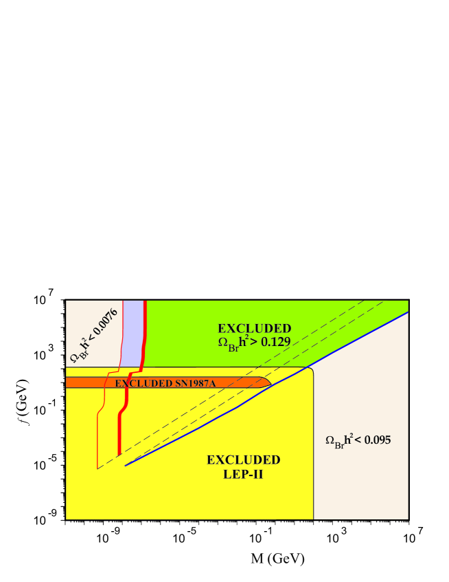
For cold branons, once we know the $c_{n}$ coefficients for the total cross section, we can compute the freeze-out value $x_{f}$ from (22) and the relic contribution to the energy density of the universe $\Omega_{Br}h^{2}$ from (23) in terms of $f$ and $M$. Imposing the observational limit on the total dark matter energy density from WMAP: $\Omega_{Br}h^{2}<0.129-0.095$ at the 95$\%$ C.L. which corresponds to $\Omega_{M}=0.23\pm 0.08$ and $h=0.79-0.65$ [1], we obtain the exclusion plots in Figs. 1 and 6.

Figure 1: Exclusion plot from cold relics abundance. The thick lines correspond to $\Omega_{Br}h^{2}=0.129-0.095$ for $N=1$ and $N=7$. Therefore the areas above the curves corresponding to $\Omega_{Br}h^{2}>0.129$ are excluded. The striped region contains the curves corresponding to $1<N<7$.

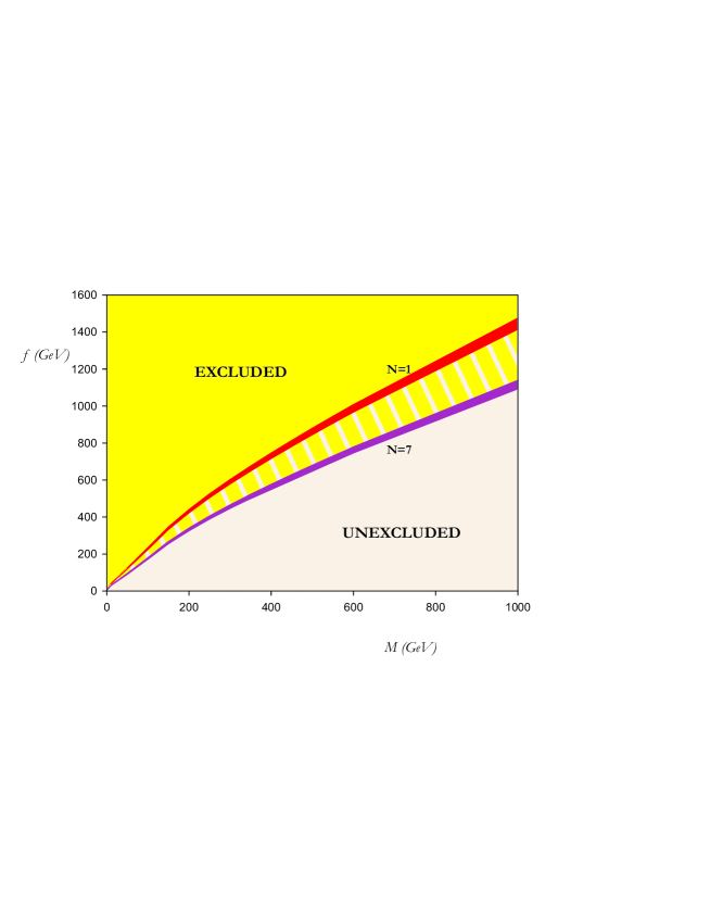
Notice that in Fig.6 we have plotted the $x_{f}=3$ curve, which limits the range of validity of the cold relic approximation. Therefore, the excluded region is that between the two curves. It is also important to note that for those values of the parameters on the solid line, branons would constitute all the dark matter in the universe.

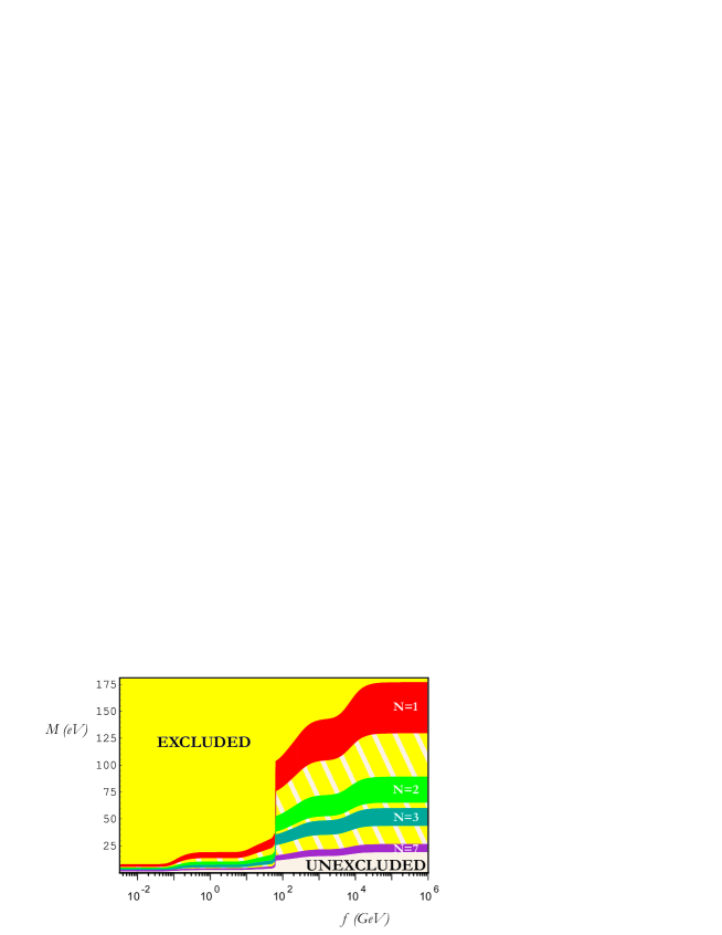
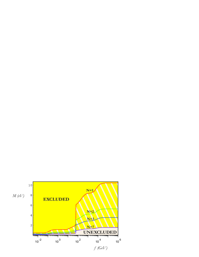
For hot branons, we have computed numerically the total annihilation rate into SM particles $\Gamma_{A}$. Using equation (20), we can find the freeze-out temperature $T_{f}$ in terms of the brane tension scale $f$. Approximately, the relation between the logarithms of these quantities is linear: $\log_{10}(f/1\mbox{GeV})\simeq(7/8)\log_{10}(T_{f}/1\mbox{ GeV})+2.8$. This expression is almost independent of the number of branons. From the numerical values of $T_{f}$ in terms of $f$, it is possible to obtain $\Omega_{Br}h^{2}$ from (21). In this case we have considered two kinds of limits. On one hand those coming from the total dark matter of the universe $\Omega_{Br}h^{2}<0.129-0.095$ in Fig. 2. On the other hand, more constraining limits on the hot dark matter energy density can be derived from a combined analysis of the data from WMAP, CBI, ACBAR, 2dF and Lyman $\alpha$ [1]. The bound reads $\Omega_{Br}h^{2}<0.0076$ at the 95$\%$C.L. and it is obtained thanks to the fact that hot dark matter is able to cluster on large scales but free-streaming reduces the power on small scales, changing the shape of the matter power spectrum. In Fig. 3 we have plotted the corresponding limits in the $f-M$ plane. Notice the abrupt jump around $f\simeq 60$ GeV in Figs. 2 and 3 (and also in Fig. 4). This $f$ value corresponds to a decoupling temperature of $T\simeq 170$ MeV which is the assumed value for the QCD phase transition. Thus, this jump is due to the sudden growth in the number of effective degrees of freedom when passing from the hadronic to the quark-gluon plasma phase. The exclusion areas depend on the number of branon species and we have plotted them for $N=1,2,3,7$ in Figs. 2,3.

Figure 2: Exclusion plot for hot relics in models with $N=1,2,3,7$ branons. For a given $N$, the shaded area corresponds to the total dark matter limit $\Omega_{Br}h^{2}=0.129-0.095$, therefore the region above such area is excluded by branon overproduction.

The validity of the previous limits requires that branons were relativistic particles at freeze-out. Therefore we require $x_{f}\ll 3$, which implies that the bounds do not work for $f<10^{-4}$ GeV. The curve $x_{f}=3$ in the hot relic case is also plotted in Fig. 6.

As commented in the introduction, in all the previous calculations we are assuming, apart from $f\ll M_{D}$, that the evolution of the universe is standard up to a temperature around $f$. In fact, the effective Lagrangian (6) is only valid at low energies relative to $f$ and therefore, it is this scale what fixes the range of validity of the results. We have checked that our calculations are consistent with these assumptions since the decoupling temperatures are always smaller than $f$ in the allowed regions in Fig. 6.

Figure 3: Exclusion plot for hot relics in models with $N=1,2,3,7$ branons. For a given $N$, the curve corresponds to the hot dark matter limit $\Omega_{Br}h^{2}=0.0076$, therefore the region above such curve is excluded by hot branon overproduction.

6 Bounds from nucleosynthesis

As commented above, one of the most successful predictions of the standard cosmological model is the relative abundance of the light elements. The calculated abundances are very sensitive to certain cosmological parameters, in particular it has been shown that the production of ⁴He increases with increasing rate of expansion $H$. From (20) we see that the Hubble parameter depends on the effective number of relativistic degrees of freedom $g_{eff}$. Usually, this number is parametrized in terms of the effective number of neutrino species $N_{\nu}=3+\Delta N_{\nu}$ as:

$$g_{eff}(T\sim\mbox{MeV})=g_{eff}^{SM}+g_{eff}^{new}\leq 10.75+\frac{7}{4}\Delta N_{\nu}$$ (36)

where $T\sim\mbox{MeV}$ corresponds to the universe temperature during nucleosynthesis. In the SM with three massless neutrino families, we have $g_{eff}^{SM}(T\sim\mbox{MeV})=10.75$ corresponding to the photon field, the three neutrinos and the electron field. In (36), in order to avoid deviations of the predicted abundances from observations, the conservative limit $\Delta N_{\nu}=1$ for the contribution from new physics is usually imposed [17], i.e. there could be only one new type of light neutrino.

Including branons, the number of relativistic degrees of freedom at a given temperature $T$ is given by:

$$g_{eff}(T)=g_{eff}^{SM}(T)+N\left(\frac{T_{B}}{T}\right)^{4}$$ (37)

where $g_{eff}^{SM}(T)$ is the contribution from the SM particles, $T_{B}$ denotes the temperature of the cosmic branon brackground and we are assuming that there are no additional new particles. If branons are not decoupled at a temperature $T$ then $T_{B}=T$, i.e. they have the same temperature as the photons. On the other hand, if they are already decoupled then its temperature will be in general lower than that of the photons. In order to calculate it, we use the fact that the universe expansion is adiabatic. Let us write:

$$h_{eff}(T)=h_{eff}^{SM}(T)+N\left(\frac{T_{B}}{T}\right)^{3}$$ (38)

where $h_{eff}^{SM}(T)$ includes only the contributions from SM particles. If at some time between branon freeze-out and nucleosynthesis, some other particle species becomes non-relativistic while still in thermal equilibrium with the photon background, then its entropy is transferred to the photons, but not to the branons which are already decoupled. Thus, the entropy transfer increases the photon temperature relative to the branon temperature. The total entropy of particles in equilibrium with the photons remains constant i.e.:

$$h_{eff}^{eq}a^{3}T^{3}=\mbox{constant}$$ (39)

and since the number of relativistic degrees of freedom $h_{eff}^{eq}$ has decreased, then $T$ should increase with respect to $T_{B}$. Thus, we find:

$$\frac{g_{eff}^{eq}(T_{f,\,B})}{g_{eff}^{eq}(T)}=\frac{T^{3}}{T_{B}^{3}}$$ (40)

where $T_{f,\,B}$ is the branon freeze-out temperature and we have used the fact that for particles in equilibrium with the photons $g_{eff}^{eq}=h_{eff}^{eq}$. Using (37), we can set the following limit on the number of massless branon species $N$:

$$\frac{7}{4}\Delta N_{\nu}\geq N\left(\frac{T_{B}}{T_{nuc}}\right)^{4}=N\left(\frac{g_{eff}^{eq}(T_{nuc})}{g_{eff}^{eq}(T_{f,\,B})}\right)^{4/3}$$ (41)

If branons decouple after nucleosynthesis we get the direct limit:

$$N\leq\frac{7}{4}\Delta N_{\nu}$$ (42)

If they decouple before, we have $g_{eff}^{eq}(T_{nuc})=10.75$, as seen before. Accordingly, we can rewrite the bound as:

$$N\leq\frac{7}{4}\Delta N_{\nu}\left(\frac{g_{eff}(T_{f,\,B})}{10.75}\right)^{4/3}$$ (43)

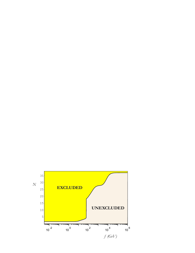
Taking $\Delta N_{\nu}=1$, the relation between the freeze-out temperature $T_{f,\,B}$ and the brane tension scale $f$ that we have obtained for hot relics can be used to get limits on the number of branons $N$ (see Fig. 4). Thus, for $f<10$ GeV, we get $N\leq 1$. This result is obtained using eq.(42) for $f<3$ GeV (which corresponds to $T_{f,B}\mathrel{\mathop{\kern 0.0pt\hbox to0.0pt{\raise 0.86108pt\hbox{$<$}\hss}}\lower 3.87495pt\hbox{\kern-1.90002pt$\sim$}}1$ MeV) or eq.(43) otherwise. However the limits are less restrictive in the range $f\simeq 10-60$ GeV. In this case we get $N\leq 3$. Above the QCD phase transition which, as commented before, corresponds to $f\simeq 60$ GeV, the bound rises so much that the restrictions are very weak. Notice that we are taking $g_{eff}^{SM}(T\mathrel{\mathop{\kern 0.0pt\hbox to0.0pt{\raise 0.86108pt\hbox{$>$}\hss}}\lower 3.87495pt\hbox{\kern-1.90002pt$\sim$}}300\;\mbox{GeV})=106.75$, i.e. we only include the minimal Standard Model matter content with a Higgs doublet and three massless neutrinos.

Figure 4: Restrictions from nucleosynthesis on the number of massless branon species $N$ as a function of $f$ for $\Delta N_{\nu}=1$.

Concerning the value of $\Delta N_{\nu}$, more constraining analysis using only BBN suggest $\Delta N_{\nu}=0.5$ [19]. However, using also WMAP results, the constraints are $N_{\nu}=2.6^{+0.4}_{-0.3}$ (95$\%$ C.L.), which are only marginally consistent with the LEP measurements of the number of neutrino families [2]. Such values would severely constrain the number of any new light particles present during nucleosynthesis. However, it has been suggested that these results could be potentially affected by systematics errors in the BBN predictions of the primordial abundances [2, 20].

7 Bounds from supernova SN1987A

Important astrophysical bounds on the brane tension scale can be obtained from the energy loss in supernovae [12]. Such energy loss is carried away essentially by light particles, i.e. photons and neutrinos if we restrict ourselves to SM particles only. However, if the branon mass is low enough, we expect branons to carry some fraction of the energy, whose importance will depend on their couplings to the SM particles. In this section, we study the constraints on $f$ and $M$ imposed by the cooling process of the neutron star in supernovae explosions. We will perform an analysis of the energy emission rate from the supernova core, similar to that done by Kugo and Yoshioka for massless branons [12]. The aim is to extend their study to arbitrary $M$ and compare with the colliders and cosmological bounds. In their work, they consider the channel corresponding to electron-positron pair annihilation. Although this contribution could be subdominant, it will allow us to get an order of magnitude estimation of the branon effect.

Figure 5: Exclusion regions from supernovae cooling by branons for $T_{SN}=10,\,50,\,70$ MeV and $N=1$. The solid lines come from the limits on the volume emissivity, and the dashed lines are the $L=10$ Km limits on the branon mean free path.

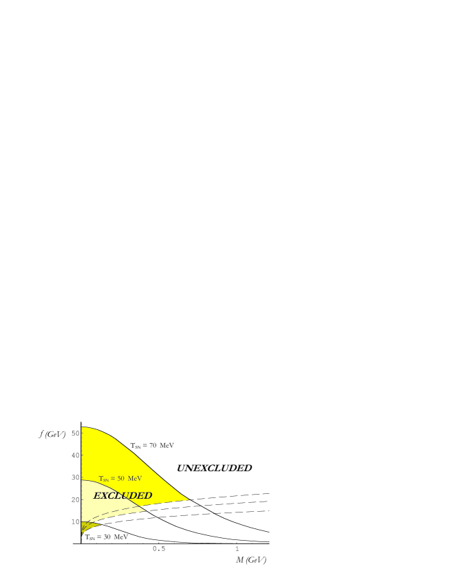
If branons are produced in the core, they can be scattered or absorbed again depending on their couplings to the SM particles. Only if the branon mean free path $L$ inside the neutron star is larger than the star size ($R\sim{\cal O}(10)$ Km), they could escape and carry the energy away. For a massive branon ($M\gg T_{SN}$), we have $L\sim(8\pi f^{8})/(M^{2}T_{SN}^{4}n_{e})$, where $n_{e}$ is the electron number density in the star. Therefore the restrictions we will obtain will be valid typically only for $f\mathrel{\mathop{\kern 0.0pt\hbox to0.0pt{\raise 0.86108pt\hbox{$>$}\hss}}\lower 3.87495pt\hbox{\kern-1.90002pt$\sim$}}5$ GeV. These restrictions appear due to the fact that the emitted energy in the form of branons could spoil the agreement between the predictions for the neutrino fluxes from supernova 1987A and the observations in the Kamiokande II [21] and IMB [22] detectors. Branons could shorten the duration of the neutrino signal if the energy loss rate per unit time and volume is $Q\mathrel{\mathop{\kern 0.0pt\hbox to0.0pt{\raise 0.86108pt\hbox{$>$}\hss}}\lower 3.87495pt\hbox{\kern-1.90002pt$\sim$}}5\times 10^{-30}$ GeV⁵. In particular, the contribution of the mentioned channel to the volume emissivity has the form:

$$Q_{Br}(f,M) \equiv \int\prod_{i=1}^{2}\left\{\frac{d^{3}k_{i}}{(2\pi)^{3}2E_{i}}2f_{i}\right\}(E_{1}+E_{2})2s\,\,\sigma_{e^{+}e^{-}\rightarrow\pi\pi}(s,f,M)$$ (44)

where $i$ refers to the electron (1) and positron (2) particles, whose masses can be neglected in the supernova core. The chemical potential in the Fermi-Dirac distribution function $f_{i}=1/(e^{(E_{i}/T-\mu/T)}+1)$ can be estimated as $\mu\sim(3\pi^{2}n_{e})^{1/3}$ with the number density of electrons: $n_{e}\sim 1.4\times 10^{-3}\;\mbox{GeV}^{3}$. With these assumptions, $Q_{Br}$ is given by:

$$Q_{Br} = \int_{0}^{\infty}dE_{1}\int_{M^{2}/E_{1}}^{\infty}dE_{2}\int_{-1}^{1-2M^{2}/(E_{1}E_{2})}d(cos)(E_{1}+E_{2})$$ (45)

$$\frac{N[2E_{1}E_{2}\left(2E_{1}E_{2}(1-\cos)-4M^{2}\right)]^{5/2}\left(1-\cos\right)^{3/2}}{{(2\pi)}^{5}\,7680\,f^{8}\,\left(1+e^{\frac{E_{1}-\mu}{T}}\right)\,\left(1+e^{\frac{E_{2}+\mu}{T}}\right)}$$

In fact, it is possible to calculate analytically the angular integral, whereas the integral over the two energies has been performed numerically. The corresponding constraints depend on the supernova temperature ($T_{SN}$) and the number of branons ($N$). In Fig. 5 we show the limits on $f$ and $M$ for $T_{SN}=30,\,50,\,70$ MeV and $N=1$.

It is interesting to note that for a branon mass of the order of the GeV, the restrictions on the brane tension scale disappear even for $T_{SN}=70$ MeV due to the limitations in the mean free path discussed above.

8 Conclusions

In this work we have studied the limits that cosmology and astrophysics impose on the brane-world scenario through the effects of massive branons. Using the effective low-energy Lagrangian for massive branons interacting with the SM fields, we have computed the annihilation cross sections of branon pairs into SM particles. From the solutions of the Boltzmann equation in an expanding universe, we have studied the freeze-out mechanism for branons and obtained their thermal relic abundances both for the cold and hot cases. Comparing the results with the recent observational limits on the total and hot dark matter energy densities, we have obtained exclusion plots in the $f-M$ plane. Such plots are compared with the limits coming from collider experiments and show that there are essentially two allowed regions in Fig. 6: one with low branon masses and large brane tensions (weak couplings) corresponding to hot branons, and a second region with large masses and low tensions (strong couplings) in which branons behave as cold relics. In addition, there is an intermediate region where $f$ is comparable to $M$, which is precisely the region studied in [13], and where branons could account for the measured cosmological dark matter.

Figure 6: Combined exclusion regions in a model with a single branon from total and hot dark matter, LEP-II single photon events [11] and supernovae cooling. The (blue) solid line on the right correspond to the cold dark matter limit. The two (red) solid lines on the left correspond to hot dark matter: the thicker one comes from the total dark matter range $\Omega_{Br}h^{2}=0.129-0.095$, whereas the thin one is the hot dark matter limit $\Omega_{Br}h^{2}=0.0076$. The two dashed lines correspond to $x_{f}=3$ for hot (upper line) and cold (lower line) dark matter.

Using the nucleosynthesis limits on the number of relativistic species, we set a bound on the number of light branons in terms of the brane tension. We see that if branons decouple after the QCD phase transition corresponding to $f<60$ GeV, the limits can be rather stringent $N\leq 3$, whereas they become very weak otherwise.

Finally, we have analysed the possibility that massive branons could contribute to the cooling of a supernova core. After estimating the energy loss rate, we again get some limits on the $f$ and $M$ parameters which are compared to the previous ones. It is shown that they are not competitive with those coming from LEP-II.

In conclusion, cosmology imposes limits on the BWS which are complementary to those coming from collider experiments and astrophysics. Although the combination of both bounds excludes an important region of the parameters space, still there are brane-world model which could be compatible with observations. Future hadronic colliders such as LHC, Tevatron-II or the planned linear electron-positron colliders, and the possibility of detecting dark matter branons directly [13] or indirectly will allow us to explore a wider region of the parameter space. Work is in progress in these directions.

Appendix A Branon production and annihilation cross sections with SM particles

In this section we present the branon production and annihilation cross sections in processes involving SM particles. The results are presented with all the internal degrees of freedom summed for the final particles and averaged for the initial ones. We have used the Feynman rules given in [11], where $N$ is the number of branons.

A.1 Scalars

$\sigma_{1}$: $\Phi^{\dagger}(p_{1}),\Phi(p_{2})\longrightarrow\pi(p_{3}),\pi(p_{4})$

$$\sigma_{1} = \frac{N}{7680f^{8}\pi s}\sqrt{\frac{(s-4M^{2})}{(s-4m_{\Phi}^{2})}}[-s(8m_{\Phi}^{2}+s)(s-4M^{2})^{2}$$ (46)

$$+(2m_{\Phi}^{2}+s)^{2}(23M^{4}-14M^{2}s+3s^{2})].$$

$\sigma_{2}$: $\pi(p_{1}),\pi(p_{2})\longrightarrow\Phi^{\dagger}(p_{3}),\Phi(p_{4})$

$$\sigma_{2} = \frac{1}{3840Nf^{8}\pi s}\sqrt{\frac{(s-4m_{\Phi}^{2})}{(s-4M^{2})}}[-s(8m_{\Phi}^{2}+s)(s-4M^{2})^{2}$$ (47)

$$+(2m_{\Phi}^{2}+s)^{2}(23M^{4}-14M^{2}s+3s^{2})].$$

The scalar results are given for a complex scalar such as charged pions or kaons. For a real scalar like the Higgs field or the neutral pion, the only change comes from the branon annihilation cross section that should be divided by two.

A.2 Fermions

$\sigma_{3}$: $\psi^{+}(p_{1}),\psi^{-}(p_{2})\longrightarrow\pi(p_{3}),\pi(p_{4})$

$$\sigma_{3} = \frac{N}{30720f^{8}\pi}\sqrt{(s-4M^{2})(s-4m_{\psi}^{2})}[(s-4M^{2})^{2}$$ (48)

$$+\frac{2m_{\psi}^{2}}{s}(23M^{4}-14M^{2}s+3s^{2})].$$

$\sigma_{4}$: $\pi(p_{1}),\pi(p_{2})\longrightarrow\psi^{+}(p_{3}),\psi^{-}(p_{4})$

$$\sigma_{4} = \frac{1}{3840Nf^{8}\pi}\sqrt{\frac{(s-4m_{\psi}^{2})^{3}}{(s-4M^{2})}}[(s-4M^{2})^{2}$$ (49)

$$+ \frac{2m_{\psi}^{2}}{s}(23M^{4}-14M^{2}s+3s^{2})].$$

These results are valid for a Dirac fermion of mass $m_{\psi}$. For massless Weyl fermions, we should multiply the branon production cross section by two, whereas the annihilation cross section should be divided by the same factor of two.

A.3 Photons

$\sigma_{5}$: $\gamma(p_{1}),\gamma(p_{2})\longrightarrow\pi(p_{3}),\pi(p_{4})$

$$\sigma_{5} = \frac{N}{7680f^{8}\pi}\sqrt{1-\frac{4M^{2}}{s}}s(s-4M^{2})^{2}.$$ (50)

$\sigma_{6}$: $\pi(p_{1}),\pi(p_{2})\longrightarrow\gamma(p_{3}),\gamma(p_{4})$

$$\sigma_{6} = \frac{1}{1920Nf^{8}\pi}\frac{s(s-4M^{2})^{2}}{\sqrt{1-\frac{4M^{2}}{s}}}.$$ (51)

A.4 $Z$

$\sigma_{7}$: $Z(p_{1}),Z(p_{2})\longrightarrow\pi(p_{3}),\pi(p_{4})$

$$\sigma_{7} = \frac{N}{69120f^{8}\pi s}\sqrt{\frac{s-4M^{2}}{s-4M_{Z}^{2}}}[3s(8M_{Z}^{2}+s)(s-4M^{2})^{2}$$ (52)

$$+(12M_{Z}^{4}+4sM_{Z}^{2}+s^{2})(23M^{4}-14M^{2}s+3s^{2})].$$

$\sigma_{8}$: $\pi(p_{1}),\pi(p_{2})\longrightarrow Z(p_{3}),Z(p_{4})$

$$\sigma_{8} = \frac{1}{7680Nf^{8}\pi s}\sqrt{\frac{s-4M_{Z}^{2}}{s-4M^{2}}}[3s(8M_{Z}^{2}+s)(s-4M^{2})^{2}$$ (53)

$$+(12M_{Z}^{4}+4sM_{Z}^{2}+s^{2})(23M^{4}-14M^{2}s+3s^{2})].$$

A.5 $W^{\pm}$

$\sigma_{9}$: $W^{\pm}(p_{1}),W^{\mp}(p_{2})\longrightarrow\pi(p_{3}),\pi(p_{4})$

$$\sigma_{9} = \frac{N}{69120f^{8}\pi s}\sqrt{\frac{s-4M^{2}}{s-4M_{W}^{2}}}[3s(8M_{W}^{2}+s)(s-4M^{2})^{2}$$ (54)

$$+(12M_{W}^{4}+4sM_{W}^{2}+s^{2})(23M^{4}-14M^{2}s+3s^{2})].$$

$\sigma_{10}$: $\pi(p_{1}),\pi(p_{2})\longrightarrow W^{\pm}(p_{3}),W^{\mp}(p_{4})$

$$\sigma_{10} = \frac{2}{7680Nf^{8}\pi s}\sqrt{\frac{s-4M_{W}^{2}}{s-4M^{2}}}[3s(8M_{W}^{2}+s)(s-4M^{2})^{2}$$ (55)

$$+(12M_{W}^{4}+4sM_{W}^{2}+s^{2})(23M^{4}-14M^{2}s+3s^{2})].$$

A.6 Gluons

$\sigma_{11}$: $g(p_{1}),g(p_{2})\longrightarrow\pi(p_{3}),\pi(p_{4})$

$$\sigma_{11} = \frac{N}{61440f^{8}\pi}\sqrt{1-\frac{4M^{2}}{s}}s(s-4M^{2})^{2}.$$ (56)

$\sigma_{12}$: $\pi(p_{1}),\pi(p_{2})\longrightarrow g(p_{3}),g(p_{4})$

$$\sigma_{12} = \frac{1}{240Nf^{8}\pi}\frac{s(s-4M^{2})^{2}}{\sqrt{1-\frac{4M^{2}}{s}}}.$$ (57)