PHENOMENOLOGY OF A SU(2) TRIPLET HIGGS

Abstract

We study the Renormalization Group (RG) evolution of the couplings in a model with a real SU(2) triplet in the Higgs sector. Insisting that the model remain valid up to 1 TeV we show that it is possible for there to be no light Higgs bosons without any otherwise dramatic deviation from the physics of the Standard Model.

1 Introduction

In this contribution we extend the study in Ref. [1] of an extension of the Standard Model in which a real scalar $SU(2)$ triplet with zero hypercharge is added to the usual scalar $SU(2)$ doublet. For details see Ref. [2]. The scalar potential of the model in terms of the usual Standard Model Higgs, $\Phi_{1}$, and the new triplet, $\Phi_{2}$, reads

$$V_{0}(\Phi_{1},\Phi_{2}) = \mu_{1}^{2}~{}|\Phi_{1}|^{2}+\frac{\mu_{2}^{2}}{2}~{}|\Phi_{2}|^{2}+\lambda_{1}~{}|\Phi_{1}|^{4}+\frac{\lambda_{2}}{4}~{}|\Phi_{2}|^{4}+\frac{\lambda_{3}}{2}~{}|\Phi_{1}|^{2}~{}|\Phi_{2}|^{2}$$

$$+ \lambda_{4}\,{\Phi_{1}}^{\dagger}\sigma^{\alpha}\Phi_{1}~{}{\Phi_{2}}_{\alpha},$$

where $\sigma^{\alpha}$ are the Pauli matrices. The expansion of the field components is

$$\Phi_{1}=\left(\begin{array}[]{c}\phi^{+}\\ \frac{1}{\sqrt{2}}\left(h_{c}^{0}+h^{0}+i\phi^{0}\right)\end{array}\right)_{Y=1},~{}~{}\Phi_{2}=\left(\begin{array}[]{c}\eta_{1}\\ \eta_{2}\\ \eta_{c}^{0}+\eta^{0}\end{array}\right)_{Y=0},$$ (6)

with $\eta^{\pm}=(\eta_{1}\mp i\eta_{2})/\sqrt{2}$ and $\phi^{0}$ is the Goldstone boson which is eaten by the $Z^{0}$. The model violates custodial symmetry at tree level giving a prediction of $\rho~{}=~{}1+4\left(\frac{\eta^{0}_{c}}{h^{0}_{c}}\right)^{2}$ for the $\rho$-parameter. In the neutral Higgs sector we have two CP-even states which mix with angle $\gamma$. The mass eigenstates $\{H^{0},N^{0}\}$ are defined by

$$\left(\begin{array}[]{c}H^{0}\\ N^{0}\end{array}\right) = \left(\begin{array}[]{cc}\cos{\gamma}&-\sin{\gamma}\\ \sin{\gamma}&\cos{\gamma}\end{array}\right)\left(\begin{array}[]{c}h^{0}\\ \eta^{0}\end{array}\right).$$ (13)

In the charged Higgs sector the mass eigenstates $\{g^{\pm},h^{\pm}\}$ are

$$\left(\begin{array}[]{c}g^{\pm}\\ h^{\pm}\end{array}\right) = \left(\begin{array}[]{cc}\cos{\beta}&-\sin{\beta}\\ \sin{\beta}&\cos{\beta}\end{array}\right)\left(\begin{array}[]{c}\phi^{\pm}\\ \eta^{\pm}\end{array}\right).$$ (20)

The $g^{\pm}$ are the Goldstone bosons corresponding to $W^{\pm}$ and, at tree level, the mixing angle is $\tan{\beta}=2\frac{\eta^{0}_{c}}{h^{0}_{c}}$. The precision electroweak data constrain $\beta$ to be smaller than about $4^{\circ}$ [1].

2 The beta-functions

In Ref. [2] the beta functions for the couplings were calculated using the one-loop effective potential [3] with $\overline{\rm MS}$ renormalization in ’t Hooft-Landau gauge and the anomalous dimensions for $h^{0}$ and $\eta^{0}$, the results read

$$\beta_{\mu_{1}} = \frac{1}{16\pi^{2}}\,\left(6\,\lambda_{4}^{2}+12\,\lambda_{1}\mu_{1}^{2}+3\,\lambda_{3}\,\mu_{2}^{2}\right)+\frac{1}{8\pi^{2}}\,\left(3\,h_{t}^{2}-\frac{9}{4}\,g^{2}-\frac{3}{4}\,{g^{\prime}}^{2}\right)\,\mu_{1}^{2},$$

$$\beta_{\mu_{2}} = \frac{1}{16\pi^{2}}\,\left(4\,\lambda_{4}^{2}+4\,\lambda_{3}\,\mu_{1}^{2}+10\,\lambda_{2}\,\mu_{2}^{2}\right)-\frac{3}{4\pi^{2}}\,g^{2}\,\mu_{2}^{2},$$

$$\beta_{\lambda_{1}} = \frac{1}{8\pi^{2}}\left(\frac{9}{16}\,g^{4}-3\,{{h_{t}}}^{4}+12\,\lambda_{1}^{2}+\frac{3}{4}\,\lambda_{3}^{2}+\frac{3}{8}\,g^{2}\,{g^{\prime}}^{2}+\frac{3}{16}\,{g^{\prime}}^{4}\right)$$

$$+ \frac{1}{4\pi^{2}}\,\left(3\,h_{t}^{2}-\frac{9}{4}\,g^{2}-\frac{3}{4}\,{g^{\prime}}^{2}\right)\,\lambda_{1},$$

$$\beta_{\lambda_{2}} = \frac{1}{8\pi^{2}}\left(6\,g^{4}+11\,\lambda_{2}^{2}+\lambda_{3}^{2}\right)-\frac{3}{2\pi^{2}}\,g^{2}\,\lambda_{2},$$

$$\beta_{\lambda_{3}} = \frac{1}{8\pi^{2}}\left(3\,g^{4}+6\,\lambda_{1}\,\lambda_{3}+5\,\lambda_{2}\,\lambda_{3}+2\,\lambda_{3}^{2}\right)+\frac{3\lambda_{3}}{8\pi^{2}}\,\left(h_{t}^{2}-\frac{11}{4}\,g^{2}-\frac{1}{4}\,{g^{\prime}}^{2}\right),$$

$$\beta_{\lambda_{4}} = \frac{1}{4\pi^{2}}\,\lambda_{4}\,\left(\lambda_{1}+\lambda_{3}\right)+\frac{3}{32\pi^{2}}\,\left(4\,h_{t}^{2}-7\,g^{2}-\,{g^{\prime}}^{2}\right)\,\lambda_{4}.$$

In the gauge and top quark sector the beta functions for the $U(1)$, $SU(3)$ and Yukawa couplings are the same as in the Standard Model and only the $SU(2)$ coupling is modified due to the extra Higgs triplet in the adjoint representation, i.e. $\beta_{g}=-\frac{5}{32\pi^{2}}\,g^{3}$.

Working with the tree-level effective potential with couplings evolved using the one-loop $\beta$ and $\gamma$ functions we are able to resum the leading logarithms to all orders in the effective potential. To carry out the RG analysis we first introduce the parameter $t$, related to $\mu$ through $\mu(t)=m_{Z}\exp{(t)}$. We perform evolution starting at $t=0$. The RG equations are coupled differential equations in the set $\left\{g_{s},~{}g,~{}g^{\prime},~{}h_{t},~{}\mu_{1},~{}\mu_{2},~{}\lambda_{1},~{}\lambda_{2},~{}\lambda_{3},~{}\lambda_{4}\right\}$. We choose rather to use the set $\left\{\alpha_{s},~{}m_{Z},~{}\sin^{2}{\theta_{W}},~{}m_{t},~{}m_{h^{\pm}},~{}m_{H^{0}},~{}m_{N^{0}},~{}v,~{}\tan{\beta},~{}\tan{\gamma}\right\}$.

Within the accuracy to which we are working, the values of the couplings at $t=0$ can be obtained from the input set using the appropriate tree-level expressions. Making use of the vacuum conditions and the notation $h^{0}_{c}\equiv v$ and $\eta^{0}_{c}~{}\equiv~{}\frac{v}{2}\,\tan{\beta}$ we can write the tree level masses as

$$m_{Z}^{2} = \frac{1}{4}\,v^{2}\,\left(g^{2}+{g^{\prime}}^{2}\right),~{}~{}m_{W}^{2}~{}=~{}\frac{1}{4}\,g^{2}\,{v}^{2}\,\left(1+\tan^{2}{\beta}\right),$$

$$m_{t}^{2} = \frac{1}{2}{h_{t}}^{2}\,{v}^{2},~{}~{}m_{h^{\pm}}^{2}~{}=~{}v\,\lambda_{4}\,\left(\cot{\beta}+\tan{\beta}\right),$$

$$m_{H^{0}}^{2} = v\,\left\{2\,v\,\lambda_{1}+\left(\lambda_{4}-\frac{1}{2}\,v\,\lambda_{3}\,\tan{\beta}\right)\,\tan{\gamma}\right\},$$

$$m_{N^{0}}^{2} = v\,\lambda_{4}\,\left(\cot{\beta}-\tan{\gamma}\right)+\frac{1}{2}\,v^{2}\,\tan{\beta}\left(\lambda_{2}\,\tan{\beta}+\lambda_{3}\,\tan{\gamma}\right),$$

with $\tan{(2\,\gamma)}=\frac{2\,\tan{\beta}\,\left(-2\,\lambda_{4}+v\,\lambda_{3}\,\tan{\beta}\right)}{2\,\lambda_{4}-4\,v\,\lambda_{1}\,\tan{\beta}+v\,\lambda_{2}\,\tan^{3}{\beta}}$. Inverting these relations we can fix the $t=0$ boundary conditions for the subsequent evolution. To ensure that the system remains in a local minimum we impose the condition that the squared masses should remain positive. We also impose that the couplings remain perturbative, insisting that $|\lambda_{i}(t)|<4\pi$ for $i={1,2,3}$ and $|\lambda_{4}|<4\pi v$. We run the evolution from $t=0$ to $t_{\rm max}=\log{(\Lambda/m_{Z})}$, with $\Lambda=1$ TeV.

3 Results in the non-decoupling regime

In the non-decoupling regime the triplet cannot be arbitrarily heavy. For this case in Fig. 1 we show the range of Higgs masses allowed when there is no mixing in the neutral Higgs sector, $\gamma=0$, for $\beta=0.04$. Such a value is interesting because it allows a rather heavy lightest Higgs (e.g. for $\beta=0.04,\;m_{H^{0}}>150$ GeV and for $\beta=0.05,\;m_{H^{0}}>300$ GeV) [1]. The strong correlation between the $h^{\pm}$ and $N^{0}$ masses arises in order that $\lambda_{2}$ remain perturbative. The upper bound on the triplet Higgs masses ($\approx 550$ GeV) comes about from the perturbativity of $\lambda_{3}$ whilst that on $H^{0}$ ($\approx 520$ GeV) comes from the perturbativity of $\lambda_{1}$. The hole at low masses is due to vacuum stability.

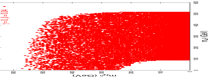
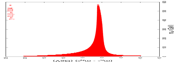
Figure 1: Allowed values of scalar masses for $\gamma=0$

The $\gamma=0.1$ case has been considered in Ref. [2] and the bounds are similar to the no-mixing case. In the maximal mixing case of $\gamma=\pi/4$ the bounds are more democratic. The largeness of $\tan(2\gamma)$ can be arranged either by tuning $2v\lambda_{1}\approx\lambda_{4}/\beta$ or by having small enough $\lambda_{1}$ and $\lambda_{4}$. In the former case, all masses are approximately degenerate. In the latter case, which corresponds to light masses, the degeneracy is lifted. The bounds for $\gamma>\pi/4$ are very similar to those for $(\pi/2-\gamma)$ on interchanging $N^{0}$ and $H^{0}$. For $\beta<0.04$ and small $\gamma$ but away from the decoupling regime the allowed regions are very similar to those for $\beta=0.04$. For larger $\gamma$, the mass bounds are again as for larger $\beta$.

4 The decoupling limit

For $\beta=\gamma=0$ there is no doublet-triplet mixing and no bound on the triplet mass. This is a special case of the more general decoupling scenario, which occurs when $|\beta+\gamma|\ll\beta$, where the triplet decouples from the doublet. For small mixing angles, the triplet Higgs has mass squared $\sim\lambda_{4}v/\beta$ and it is possible to have $\lambda_{4}\sim v$ by keeping $\mu_{2}^{2}$ large. In this case $\beta+\gamma\approx 0$ [2]. This is the decoupling limit in which the triplet mass lies far above the mass of the doublet and the low energy model looks identical to the Standard Model.

5 Conclusions

We have computed the one-loop beta functions for the scalar couplings in an extension to the Standard Model which contains an additional real triplet Higgs. Through considerations of perturbativity of the couplings and vacuum stability we have identified the allowed masses of the Higgs bosons in the non-decoupling regime [2]. In the decoupling regime, the model tends to resemble the Standard Model. The near degeneracy of the triplet Higgs masses ensures that, at least for small $\gamma$, the quantum corrections to the $T$ parameter are negligible (the $S$ parameter vanishing since the triplet has zero hypercharge) [1]. This means that the lightest Higgs boson can be heavy as a result of the compensation arising from the explicit tree-level violation of custodial symmetry and it is possible to be in a regime where all the Higgs bosons are heavy without any dramatic deviation from the physics of the Standard Model.

References

• [1] J. R. Forshaw, D. A. Ross, B. E. White, JHEP 0110 (2001) 007.
• [2] J. R. Forshaw, A. Sabio Vera, B. E. White, to be published in The Journal of High Energy Physics, hep-ph/0302256.
• [3] S. R. Coleman and E. Weinberg, Phys. Rev. D 7 (1973) 1888; R. Jackiw, Phys. Rev. D 9 (1974) 1686; J. Iliopoulos, C. Itzykson and A. Martin, Rev. Mod. Phys.  47 (1975) 165; B. Kastening, Phys. Lett. B 283 (1992) 287; C. Ford, D. R. Jones, P. W. Stephenson and M. B. Einhorn, Nucl. Phys. B 395 (1993) 17; M. Quiros, Helv. Phys. Acta 67 (1994) 451.