LU TP 03-32
hep-ph/0307044
revised October 2003
Scalar Form Factors in SU(3) Chiral Perturbation Theory
Johan Bijnens and Pierre Dhonte
Department of Theoretical Physics, Lund University
Sölvegatan 14A, S 22362 Lund, Sweden
The scalar form factors for the pions and kaons are calculated in SU(3) Chiral Perturbation Theory at order , in the isospin limit . We find in general sizable corrections of . We use our results to obtain information on the suppressed low energy constants and as well as on two low energy constants. We present some numerical results for masses and decay constants as well.
We derive a relation for the scalar form factors analogous to Sirlin’s relation for vector form factors.
1 Introduction
Chiral Perturbation Theory (ChPT) in its effective Lagrangian form was introduced by Weinberg [1] and developed into its standard form, for both two and three light flavours (referred to as and ) formalisms, up to order , by Gasser and Leutwyler [2, 3]. The underlying assumption of ChPT is that the chiral symmetry present in the QCD Lagrangian is spontaneously broken to its vector subgroup, . This breaking is due to the finite quark condensates111See below for the alternative view of generalized ChPT.
| (1.1) |
The quark and gluon degrees of freedom are integrated out and replaced by pseudo-scalar fields representing the lightest pseudo-scalar mesons triplet () or octet (), these are the Goldstone bosons resulting from the spontaneous chiral symmetry breaking. Introducing non-zero quark masses renders the chiral symmetry only approximate. This results in masses for the mesons.
ChPT is thus an effective theory of QCD, perturbatively expanded in powers of the relevant momentum and the quark masses, and is non-renormalizable. Loop corrections produce ultra-violet divergences which require the introduction of new counterterms and associated low energy constants (LEC) at each order in the parameters expansion. The number of new operators is, however, finite at each order, allowing ChPT to be predictive. Recent introductions to ChPT can be found in Ref. [4].
A basic set of calculations in ChPT at order was performed in [3, 5] and used to determine the LEC at order , the , to that order. and were assumed to be negligible there using the large limit of QCD [6]. This assumption was studied at order in [7] by considering scalar form factors and a scalar two-point function.
The state of ChPT in the meson sector now is such that many calculations have been pushed to the next order, or next-to-next-to-leading (NNLO) or two-loop order. There are two main reasons to explore the two-loop region of Chiral Theory. First, the accuracy of experimental results has improved so this accuracy is now routinely needed and we need to determine all LECs to the required precision. Second, spontaneous chiral symmetry breaking of QCD does not have to be driven by the quark condensates, Eq. (1.1). An alternative bookkeeping method in the Lagrangian expansion might be necessary, leading to a Generalized ChPT (GChPT), see Ref. [8] and references therein. The combination of the two-loop calculation of -scattering in ChPT [9, 10], together with the dispersive Roy equation analysis [11], lead to sharp predictions for the scattering lengths [12] confirmed by the E865 experiment [13] leading to the conclusion that ChPT is indeed driven by the quark condensate [14]. See also [8, 15, 16] for relevant discussions. In the case of ChPT the possibility of a small quark condensate is not ruled out [7, 17, 18]. The pion scalar form factor has been evaluated to order in ChPT in [19] after earlier dispersive work [20].
The two-loop calculations in ChPT of the masses [21, 22] indicated the possibility of sizable NNLO corrections. This behaviour persisted when the calculations also included [23, 24] such that the could be determined with accuracy under similar assumptions as the determination [3]. In [24] a search was done for possible values of and that would lead to acceptable convergence of all quantities considered there. In [25] effects of isospin violation in the masses were taken into account also to order as well as well as the new E865 data of [13].
This paper consists of two major parts. In the first part we calculate the scalar form factors of pions and kaons to order in ChPT and show some numerical results for the sizes of the various contributions to the different form factors. We therefore first present the framework of ChPT in the isospin limit and including external scalar fields in Section 2 and sketch the calculation of the scalar form factors in Section 3. The analytical results of this calculation are given in Section 4.1 and App. B. In Section 4.3 we present a series of plots allowing the reader to judge the importance of the different parts of the calculations. One result of more general interest is that the curvature of the scalar form factor in decays [26] can in principle be determined from the quantities considered here. Unfortunately as discussed at the end of Sect. 5.5 the numerical accuracy obtainable is rather low.
Those results allow us then to proceed to the second major part of this paper. A study of the form factors allowing to relax some of the assumptions made in the previous determinations and the effects of these assumptions on the scalar form factors. We made use of dispersive analysis, Section 5.1, to extract experimental information. This allows us to obtain extra numerical results for some of the LEC’s of the theory, Sections 5.3 and 5.5. We also present some updated results on masses and decay constants in Sect. 5.6.
A third result is a relation between the scalar form factors that has only second order corrections in quark mass differences. This relation, Eq. (3.18) is proven in general in App. A and is valid for all where an expansion in mass differences is valid. It is the analog of the relation derived by Sirlin for the vector form factors [27].
2 The ChPT Lagrangian
This section contains a very short overview of ChPT and serves also to define our conventions. More detailed introductions can be found in [4]. The Lagrangians of ChPT are ordered in the counting, powers of momenta (), quark masses or external scalar or pseudo scalar fields () and external vector or axial-vector fields (). We keep to the three flavour case here.
The Lagrangian for the strong and semi leptonic mesonic sector to NNLO can be written as
| (2.2) |
where the subscript refers to the chiral order. The lowest order Lagrangian
| (2.3) |
The mesonic fields enter via
| (2.4) |
and the quantity introduces the external vector () and axial-vector () currents
| (2.5) |
while the scalar () and pseudo scalar () currents are contained in
| (2.6) |
The or NLO Lagrangian was introduced in Ref. [3] and reads
| (2.7) | |||||
The and terms introduce also the field strength tensor
| (2.8) |
The two terms proportional to and are contact terms and do not enter physical amplitudes. In the present case, we keep only the relevant scalar current interactions from which we extract and separate the quark masses contribution:
| (2.9) |
We quote the schematic form of the NNLO Lagrangian in the case
| (2.10) |
and refer to [28], where this was first constructed after the earlier attempt of [29], for the full expressions. The last four terms are contact terms [28].
All ultra-violet divergences produced by loop diagrams of order and cancel in the process of renormalization with the divergences extracted from the low energy constants ’s and ’s. We use here dimensional regularization and the standard modified minimal subtraction version used in ChPT. An exhaustive description of the regularization and renormalization procedure including a description of the freedom involved can be found in Ref. [10] and [30].
The subtraction of divergences is done explicitly by
| (2.11) |
and
| (2.12) |
where and are defined by
| (2.13) |
| (2.14) |
The coefficients , and are constants while the ’s are linear combinations of the ’s. Their explicit expressions can all be found in [30] where they have been calculated in general.
Scalar form factors can be calculated using functional derivatives w.r.t. the external scalar field [3].
3 The scalar form factors: definitions and overview of the calculation
3.1 Definitions
The scalar form factors for the pions and kaons are defined as follows:
| (3.15) |
with and being indices in the flavour basis and , a meson state with the indicated momentum.
In the present case of isospin symmetry , the various pion scalar form factors obey
| (3.16) |
The kaon currents are related by the following rotations in flavour space
| (3.17) |
The other scalar form factors can be related to these using charge conjugation and time reversal. In (3.1) and (3.1) we have also given the notation we shall use for the form factors in the remainder.
The scalar form factor is proportional to the form factor used in decays.
The scalar form factors can be shown to obey a relation similar to the Sirlin [27] relation for the vector form factor
| (3.18) |
The proof of this relation is in App. A.
The values at zero momentum transfer are related to the derivatives of the masses w.r.t. to quark masses because of the Feynman-Hellman theorem (see e.g. [5])
| (3.19) |
This also shows that we can expect large corrections at . The argument is fairly simple. If
| (3.20) |
then
| (3.21) |
So we see that in the scalar form factors the relative corrections can get enhanced by factors of order 3 compared to the masses.
3.2 Diagrams
The relevant diagrams for the present case are identical to those involved in the electromagnetic form factors [31] with the electromagnetic current replaced by the scalar one. We list the diagrams appearing at each order but refer to [24, 31] for a deeper discussion of the checks to perform and the renormalization.
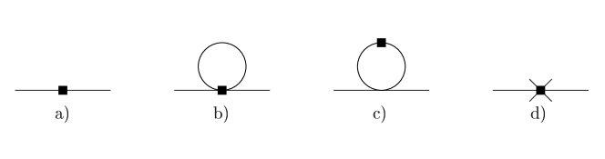
3.2.1 Leading and next-to-leading orders
The diagrams are shown in Fig 1. The black square represents an external scalar insertion from - diagram a) - and the crossed square a scalar insertion form - diagram d). Also included, are the tadpole contributions with two possible insertions.
The lowest order contributions are
| (3.22) |
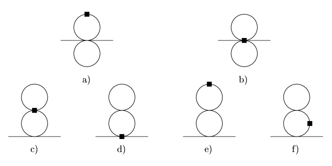
3.2.2 Next-to-next-to-leading order
There are four distinct topologies involved in order diagrams. Firstly, the two loop diagrams, built exclusively on vertices, are represented in Fig 2. There again does a black square represent a scalar interaction.
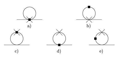
Secondly, one loop diagrams can contribute, with one vertex built on , possibly including a scalar insertion. These are represented in Fig 3.
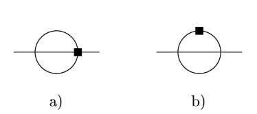
There are also sunset integrals and irreducible contributions to include through the non-factorizable diagrams of Fig 4. See [21] and [31] for a treatment of sunset integrals and irreducible two loop integrals.
Of course, one must finally include the tree contribution, Fig 5.

4 Analytical and First Numerical Results
4.1 Analytical expressions - LEC’s
We present here the dependence of all the scalar form factors on the LECs of order . It can be easily checked that the relation (3.18) is satisfied.
| (4.23) | |||||
| (4.24) | |||||
| (4.25) | |||||
| (4.26) | |||||
| (4.27) | |||||
4.2 Loop corrections
We present only the results for . The expressions for the others are obtainable on request from the authors. Form factors including external etas can be calculated as well if required. The order results are in agreement with those of [5]. The form given in App. B is the one that corresponds to the expressions we use and which can also be found in App. B.
4.3 First Numerical Results
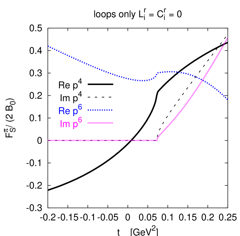
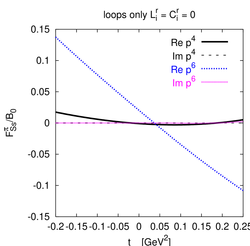
In this part we present some plots of the sizes of the various corrections for the case with , we have used the values of [25], fit 10, and the neutral pion, neutral kaon and physical eta masses as well as MeV and MeV. These plots are included here to show the relative sizes of the many contributions to the scalar form factors we have calculated. These corrections are in many cases large as expected from the argument given at the end of Section 3.1.
In Fig. 6a we have plotted the loop contributions to the pion scalar form factor normalized to . The order is then one. The two-loop contribution in this case is sizable but not enormously so. The loop contributions to the pion strange scalar form factor, , are plotted in Fig. 6b. The corrections here are moderate. Note that the imaginary part vanishes at order and remains small at . This was expected since it requires a kaon or eta loop when the LECs are set to zero.
(a)
(b)
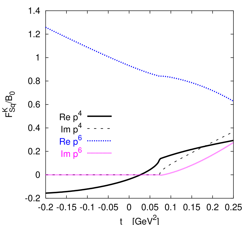
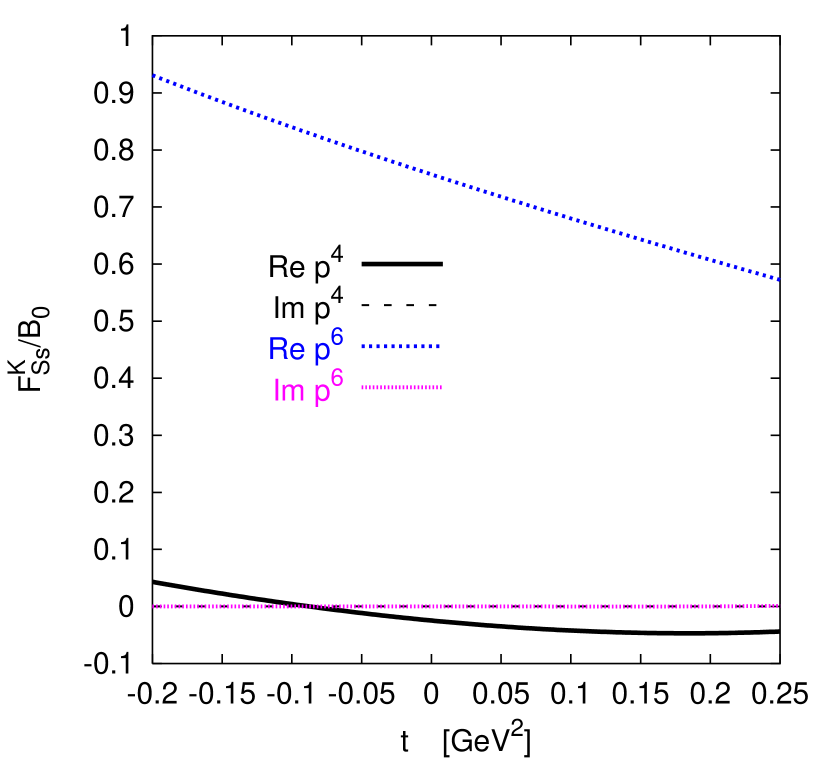
In Fig. 7a we have plotted the loop contributions to the kaon light quark scalar form factor normalized to . There are large two-loop contributions in this case for the real part while the imaginary part has only modest corrections. This agrees with the imaginary part calculated previously in [32].
The kaon strange scalar form factor, , is plotted in Fig. 7b. The corrections here are also large compared to the order result which is 1. The imaginary parts vanish at order and remain very small at order .
(a)
(b)
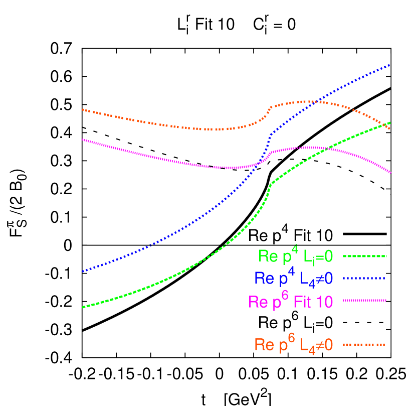
We will do a more extensive analysis in the next section but here we want to show the effects of the diagrams involving separately. We use here the of fit 10 of [25], the and the other input parameters as given above. We also present the dependence on by changing it from zero to keeping the others at the values given by fit 10.
In Fig. 8a we plotted the effect of the on compared to the case with the . The curves are for the real parts at order and order . The curves are labelled respectively Fit 10, and . Notice that the effect of such a small is fairly large.
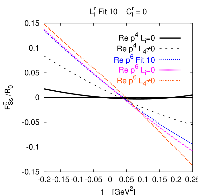
The pion strange scalar form factor, is shown in Fig. 8b. At order only contributes but it has a large effect. contributes as well but is assumed zero. So there is no difference for this case for Fit 10 and the . Notice that the effect of the corrections is larger than the change due to this value of . It is therefore necessary to include the effects before drawing conclusions on the values of and .
(a)
(b)
We can present similar plots for the dependence of the kaon scalar form factors but the conclusions are qualitatively the same as for the pion form factors.
5 Numerical Analysis
5.1 Dispersive Inputs
There is no direct experimental measurement of the scalar form factors but information can still be extracted from elastic scattering experiments. We recall here the principal results of dispersive analyses and refer to [33] and [7] for a more thorough treatment. An analysis within a unitarized model approach can be found in [34].
5.1.1 The Muskhelishvili-Omnès (MO) problem
We consider first the one channel case, i.e. where only pion interactions are considered. The problem of finding the functions satisfying the pion form factor’s analytical properties is referred to as the Muskhelishvili-Omnès problem. Provided some convergence conditions on the form factor and the phase shift are satisfied, the solution is of the form:
| (5.28) |
Watson’s theorem then relates the phase shift to the scattering phases , here . This can be extended to two or more channels. We restrict here to the two channel case, and in the isospin and angular momentum zero case, -wave. The MO problem becomes a system of coupled equations of the two independent contributions
| (5.29) |
where is an isospin zero operator, e.g. . The interesting feature of the MO solution is the possibility to write the general solution using two independent sets of solutions fulfilling the initial conditions
| (5.30) |
and this independently of the exact form of the operator . The solution is then built on the value of the form factors at the origin:
| (5.31) |
5.1.2 The solutions
The method and coding of the solutions were borrowed from Moussallam [7, 35], where the solutions are obtained by solving the linear system of equations – equivalent to (5.28) for the two channel case – given by the discretized form of
| (5.32) |
and
| (5.33) |
where
| (5.34) |
and are the T-matrix elements of the needed , scattering channels. Three T-matrix models of scattering are used, from Au et al. [36], Kamiński et al. [37] and Ananthanaryan et al. [35], and we refer again to [7, 35] for details and differences.
| Au(1) | 1. | 2.33 | 9.94 | 0. | 0.92 | 5.31 |
|---|---|---|---|---|---|---|
| Au(2) | 0. | 0.31 | 1.03 | 1. | 0.78 | 0.98 |
| lm(1) | 1. | 2.43 | 10.28 | 0. | 0.75 | 3.49 |
| lm(2) | 0. | 0.27 | 0.93 | 1. | 0.84 | 1.00 |
| Abm(1) | 1. | 2.45 | 10.61 | 0. | 1.03 | 5.36 |
| Abm(2) | 0. | 0.21 | 0.72 | 1. | 0.81 | 0.98 |
The results of our calculation for the different derivatives of the canonical solutions using the programs of [7, 35] at the origin are presented in Table 1. We have only used the last solution, since they use a better physical model for the to amplitude and newer phases.
Similar work exists for the form factor, , in [38]. We have not obtained their results in a form we can use in the same way.
5.2 Other experimental inputs and Values of the ,
The other experimental inputs are the same as those used in [25] corresponding to fit 10 there. This differed from the main fits reported there by using the then preliminary data of [13].
We would like to study the dependence on and as well. A study was already performed in [24] where we varied the input assumptions of and and then refitted the other . We have redone this now with the data of [13] included, so we use all the inputs described above with as input values for and values on the grid
| (5.35) |
In all these cases we have used the resonance saturation contributions to the constants of order as derived in [24] and those for the decay constants and the masses as derived in [21] but we have chosen the value of as defined in [21] to be zero. This is also the choice made in [24]. The reason for this is that the estimate of the parameter of [21] was very uncertain and the naive value obtained there led to contributions to the masses which were enormous.
Fits of a quality similar to the one with could be obtained for most points on the grid (5.35). All those satisfying
| (5.36) |
had a value of below 1. The precise definition of the can be found in [24, 25]. The data used up till now do not allow for a determination of and . But note that while these cannot be determined, a given assumption on their value leads to correlated values of all the other in order to obtain a decent fit to the data. This effect is taken into account in the next subsections.
In the numerical results quoted below we have used the neutral kaon and pion masses and a subtraction scale MeV.
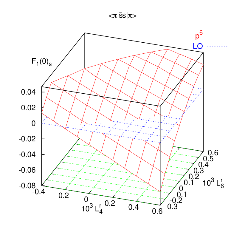
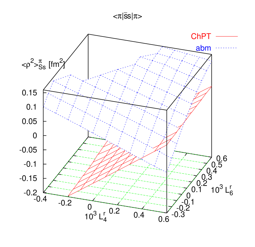
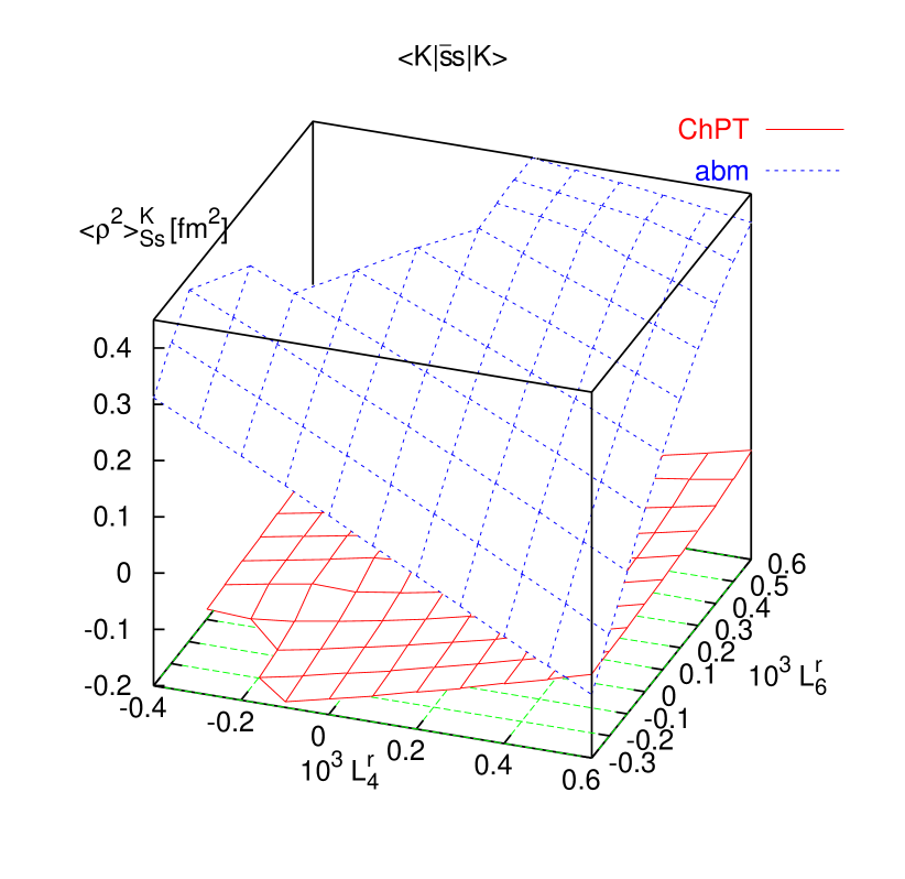
5.3 Variation with and of the scalar form factors at .
It should be kept in mind that the values of the other used change as well with the values of and in accordance with the fit to the other experimental values as described in Section 5.2. The contributing to the scalar form factors are set to zero here.
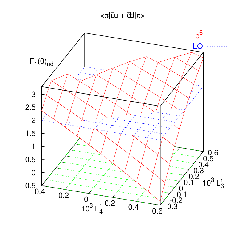
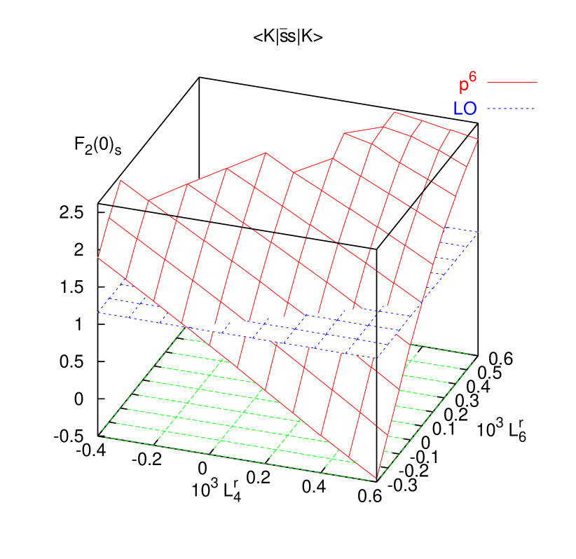
We first show the results for in Fig. 9a. We also show the lowest order expectation of 2 for comparison. Only the points with good fits are shown.
(a)
(b)
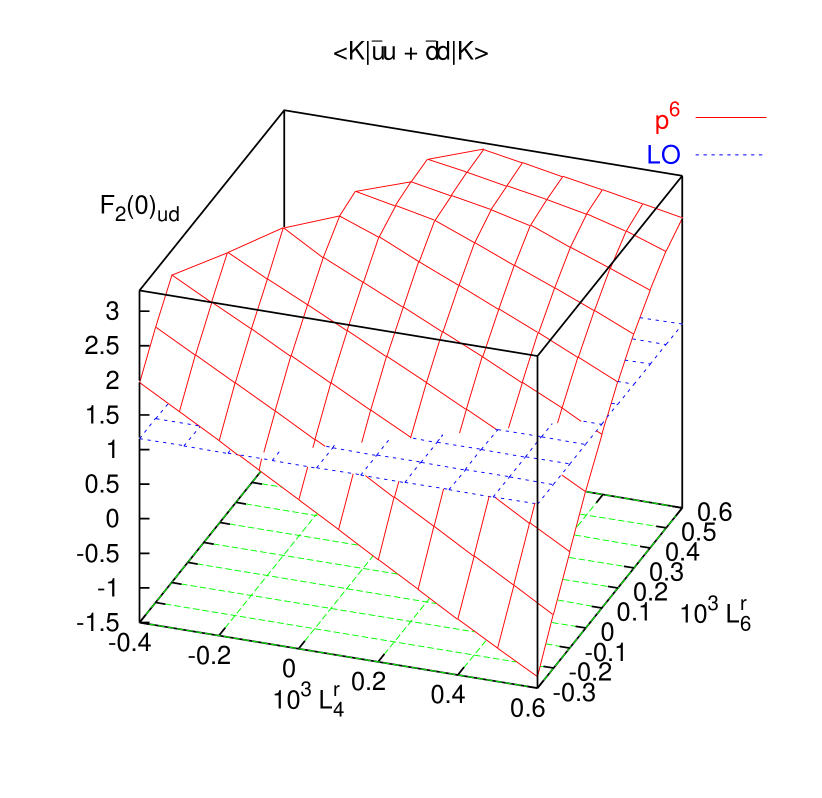
We show similarly in Fig. 9b the value of together with the lowest order value of . Notice that in both cases the corrections are large for most values of and but reasonable in the region of the axis . Requiring the corrections to be of a reasonable size thus leads to constraints on and .
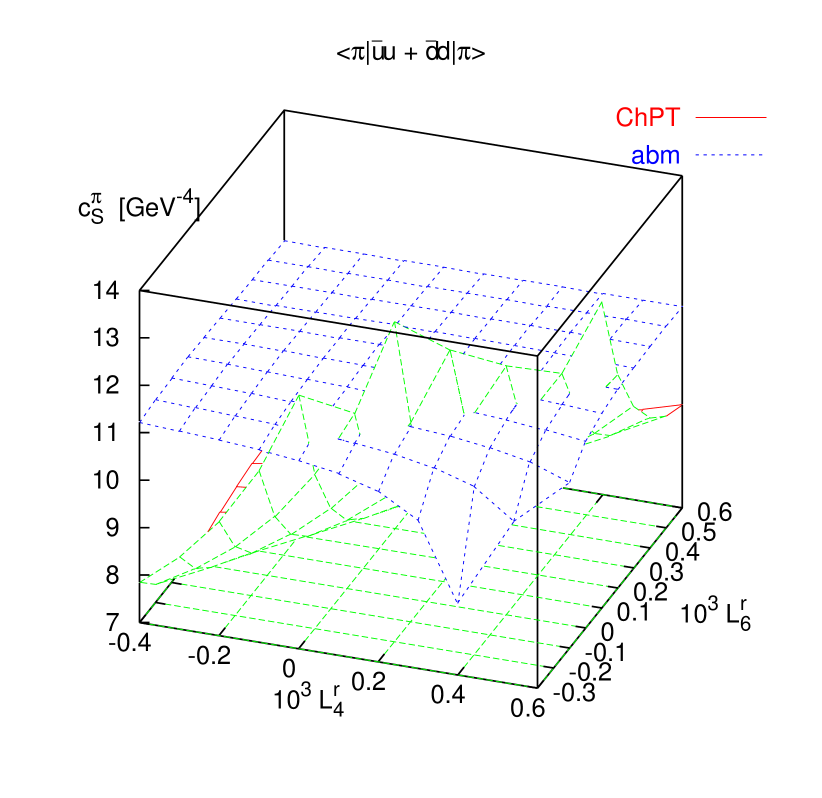
We have also studied the current. The results for the pion case are shown in Fig. 10a. The result for is shown in Fig. 10b. Notice that the strange quark content in the pion remains small for the entire studied region.
(a)
(b)
At this point we cannot determine the values of and but there is also a tendency in those two cases for the corrections compared to the lowest order to be small for positive and a correlated value for along .
5.4 Slopes and the value of and
We can use our results to get at the form factors away from zero in two different ways. First we can of course simply use our full ChPT calculation to calculate them to order using the input values of and and the resulting fitted values of the other .
Second, from Sect. 5.1 we can calculate the form factors at given the values at zero, this uses then all the dispersive constraints.
We then require that both methods give the same results and obtain in this way constraints on the values of and . The main effect of this comparison can already be studied by looking at the radii only since for the curvature we expect a larger effect from the . We still assume here that the for those contributing to the radii.
The results for the pion scalar radius,
| (5.37) |
are shown in Fig. 11a. We have normalized here to the value at zero. That leads to singular predictions when vanishes, but away from that region the dispersive prediction is quite stable and is entirely predicted by the values of the phase shifts. It is fully dominated by the first independent solution of the MO equations. The ChPT prediction is quite dependent on and The two agree for positive values of and a correlated value of .
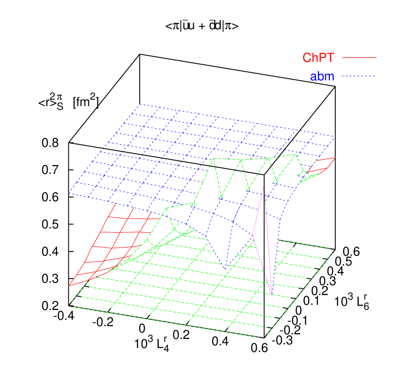
(a)
(b)
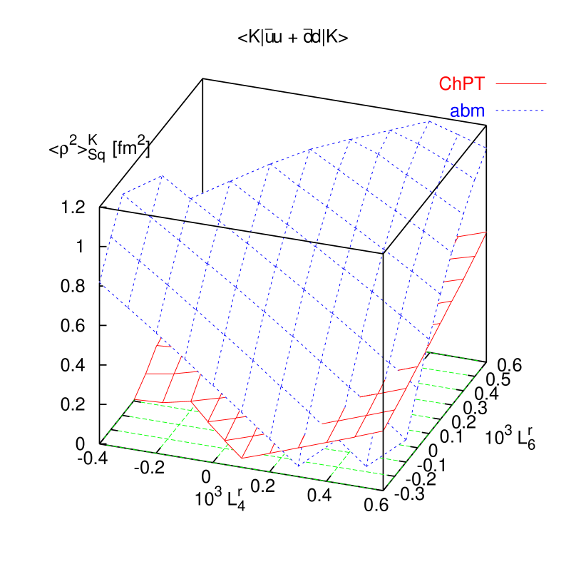
The results for the kaon light quark scalar radius,
| (5.38) |
are not as easily shown, as the calculated value of runs through zero in the relevant region, producing strong effects in both the dispersive and ChPT results. We plot instead the scalar radius normalized to the lowest order result
| (5.39) |
This is shown in Fig. 11b. The dispersive prediction is less stable here. The relative strength of the two canonical MO solutions varies much more than in the pion case. This has a strong effect since both solutions have a very different radius, as can be seen by comparing the first derivatives columns in Table 1.
Notice that the agreement between the chiral and dispersive radii tend to be in the same region of and where the corrections to the lowest order results for the form factors at are fairly small, as discussed in the previous subsection, taking into account that the results are less reliable in the kaon case.
The strange quark scalar current can be studied in exactly the same way. The pion strange scalar form factor has a very small value at zero, we normalize therefore to the value and plot
| (5.40) |
The results are shown in Fig. 12a both for the dispersive and the ChPT result. Again the dispersive result shows a significant variation with and since both solutions of the MO equations are important and their contributions vary significantly depending on the values of and .
(a)
(b)
The prediction for the kaon strange quark radius
| (5.41) |
is stable for most values of the , except for a region near the top of the and the bottom of the range where is near zero. The reason is that for most input values the second MO solution dominates. The two predictions never agree, the dispersive estimate is positive and the ChPT one is negative. We plot instead
| (5.42) |
in Fig. 12b. For this quantity there is a small region of overlap between the dispersive and the ChPT estimates but it is where is near zero and we can have a large sensitivity to effects from the .
It is somewhat difficult to get a final conclusion about and since the effect of the constants has to be evaluated. This requires a general study of effects in the scalar sector which goes beyond the scope of this paper.222The analysis might be doable by extending some of the lines of work of [39]. The main constraint from the pion scalar radius is
| (5.43) |
To be precise, this is the curve where the two surfaces shown in Fig. 11a intersect. If in addition we require that the values of the scalar form factors at zero do not deviate too much from their lowest order values we obtain that should be in the range from to . The latter requirement means staying close to the intersection of the two surfaces in Fig. 9a.
We have shown several numerical results in Table 2 for grid points in this region.
5.5 Curvatures and the value of and
Since the values at zero determine the form factors away from zero, we can also compare higher order terms in the expansion in . Because of the large corrections to the values at zero coming from order , there is a rather large uncertainty in the resulting values. We have therefore not done a full error analysis.
We define the pion scalar curvature via
| (5.44) |
The results both from the dispersive and the ChPT analysis are shown in Fig. 13a. It should be remarked that, precisely as in the two flavour case analyzed in [19] a large part of the curvature is due to the loop effects and the contribution from the constants is not the dominant one. This can be seen by looking at the scale in Fig. 13a. The difference between the ChPT prediction with the and the dispersive result is small.
The same analysis can be performed for the other form factors. We again run into the problem of normalizing the curvature, just as we had for the slopes. For the rest we use thus quantities normalized to . We show the pion strange scalar curvature
| (5.45) |
in Fig. 13b. The variation of the dispersive result is large here again due to the fact that both MO solutions contribute with a strong variation in relative strength.
(a)
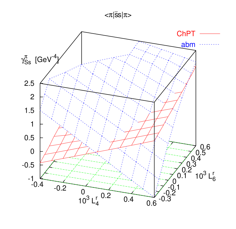
(b)
The curvatures can now be used to estimate combinations of the . We get
| (5.47) |
From the figures 13a and 13b it is obvious that the extracted values will depend strongly on the input values used for and , since the difference between the surfaces in those figures gives the values of the . On the other hand, we see that there are several ways to extract the same quantities. It turns out that these tend to give similar values in the region of preferred in the previous subsections. Away from these regions, the obtained values for the are much larger than naive order of magnitude estimates.
| Set | Fit 10 | A | B | C |
|---|---|---|---|---|
| 0.0 | 0.4 | 0.5 | 0.5 | |
| 0.0 | 0.1 | 0.1 | 0.2 | |
| (ChPT, ) | 2.54 | 1.99 | 1.75 | 2.12 |
| (ChPT, ) | 0.020 | 0.004 | 0.002 | 0.008 |
| (ChPT, ) | 1.94 | 1.36 | 1.12 | 1.51 |
| (ChPT, ) | 1.77 | 1.35 | 1.17 | 1.45 |
| (fm2) | 0.617 | 0.612 | 0.610 | 0.614 |
| (fm2) | 0.384 | 0.547 | 0.625 | 0.563 |
| 2.6 | 0.56 | 0.55 | 0.71 | |
| 3.3 | 0.55 | 0.48 | 0.75 | |
| 0.55 | 0.11 | 0.33 | 0.15 | |
| 0.56 | 0.02 | 0.15 | 0.03 | |
| 4.1 | 0.27 | 0.99 | 0.08 | |
| 1.5 | 0.52 | 0.26 | 0.78 | |
| 1.1 | 0.84 | 0.12 | 1.3 | |
| (MeV) | 87.7 | 63.5 | 70.4 | 71.0 |
| 0.136 | 0.230 | 0.253 | 0.254 | |
| 0.083 | 0.226 | 0.059 | 0.048 | |
| 0.169 | 0.157 | 0.153 | 0.159 | |
| 0.051 | 0.063 | 0.067 | 0.061 | |
| 0.736 | 1.005 | 1.129 | 0.936 | |
| 0.006 | 0.090 | 0.138 | 0.043 | |
| 0.258 | 0.085 | 0.009 | 0.107 | |
| 0.687 | 0.938 | 1.055 | 0.874 | |
| 0.007 | 0.100 | 0.149 | 0.057 | |
| 0.306 | 0.162 | 0.094 | 0.183 | |
| 0.734 | 1.001 | 1.124 | 0.933 | |
| 0.052 | 0.151 | 0.197 | 0.104 | |
| 0.318 | 0.150 | 0.073 | 0.171 |
We have collected in Table 2 various results for four sets of . The first one is exactly the same as fit 10 of Ref. [25] and all quantities coincide with the one reported there. The notation used in Table 2 means that the quantity is determined from using the as determined from a fit to the same experimental input as used in fit 10 in Ref. [25] but with the values of and as indicated. The difference between the first two determinations of is due to the difference from from .
The three other sets - A,B, and C - of were generated by different sets of and in the agreement region of the two previous sections, and . The extracted constants are generally similar over the three sets but still show a dependence on and . There are particular disagreements on values obtained via and . For the former, we can, as we did for the light quark scalar radius, attribute the variations over the extracted values to the construction of on the canonical MO solutions. For , the argument is similar, as now the relative strength of the MO solutions is compensated by the values of and .
A final conclusion on the value of which is needed for the measurement of [26] is not very easy since it depends so strongly on the values of and as well as on which dispersive quantities are used to evaluate it.
5.6 Masses and Decay Constants
For completeness we present here results for the masses and decay constants for the sets of input parameters we use. These can also be found in Table 2. We present results for
| (5.48) |
Notice that in [25] the corresponding numbers were quoted for the “Main Fit” which used the old data.
A glance at Table 2 shows that the pion decay constant in the chiral limit can be substantially different from the value of about MeV for the case of fit 10.
We would like to remind the reader that from within ChPT all the solutions shown in the table are good fits to all fitted experiments. The new sets are preferred under the assumptions that the contributing to the scalar form factors and masses vanish as well as the constraints from assuming the corrections to the scalar form factors at zero to be small.
6 Conclusions
In this paper we have computed the full order expressions in Chiral Perturbation Theory in the isospin limit for all pion and kaon scalar form factors. This is described in the first major part of this paper. In addition we have shown various numerical results that allow the reader to get a feeling for the size of the various contributions.
We also found a new relation between the scalar form factors, analogous to the Sirlin relation for vector form factors.
This calculation is important for future determination of the LEC’s and in the absence of a better knowledge of these constants the precision on numerical results is limited.
In the second major part of this paper we have used the experimental input used in the previous fits of the order LECs and refitted the as a function of the input values of and showing that a rather wide range of these leads to good fits to the included data. We also used the solutions of the Muskhelishvili-Omnès problem for the scalar form factors with as input the known and scattering phases. This allowed to study the scalar radii and curvatures as a function of and and obtain consistency relations between them. Under the assumptions of vanishing contributions to the scalar form factors at and the scalar radii these consistency requirements together with the assumption that the corrections to the scalar form factors at zero should be small, there is a preferred region of and around and . In Table 2 we have shown the values of several quantities in this region.
We have used our results for the curvature to obtain constraints on two order constants, and . These are of the expected naive order of magnitude but the precision obtained is rather low.
Acknowledgements
Appendix A The proof of the symmetry relation
The relation for the scalar form factors, Eq. (3.18) can be proven using the same method as used in the second paper of Ref. [27] when the different behaviour of scalar and vector currents under charge conjugation is taken in to account.
We write the Hamiltonian in the form
| (A.1) |
is the Hamiltonian in the limit . We now do oldfashioned perturbation theory in , and look at the variation of
| (A.2) |
w.r.t. at . This can be rewritten as an expectation value involving the and field, and . Applying the operator with the second generator of -spin and charge conjugation we obtain that
| (A.3) |
while charge conjugation and the fact that it is a scalar current require the full form factors in (A.3) to be equal. The first variation w.r.t. of thus vanishes.
The same argument can be applied to the combination
| (A.4) |
and in the -spin limit both combinations are related. This relation can be brought into the form of Eq. (3.18) using isospin.
Appendix B Analytical expressions for
For brevity we only write the pion scalar form factor with the light quark densities. The expressions for the others can be obtained from the authors. The integrals can be found in several places. The functions , ,…can be found in [21] and [24]. The ,…are defined in [21] and the can be found in [31]. The method to evaluate the was developed in [21] and the are evaluated as described in [31] using the methods of [41].
The result given is not the shortest possible analytical one. There are various relations between the integrals that we have not implemented. The reason is that these relations involve inverse powers of and we have used simplifying relations to rewrite all the masses in the numerators in terms of and . This has as a consequence that, if we had used those relations, the numerators of the poles would not cancel exactly numerically and produce possible instabilities for small .
We write the pion scalar form factor as
| (B.5) |
The superscript indicates the chiral order. The lowest order is simply
| (B.6) |
The next order has been calculated in [5] and we agree with their result, it is
| (B.7) | |||||
The next order we split in several different parts
| (B.8) |
The result for can also be found in the main text we simply repeat it here for completeness.
| (B.9) | |||||
| (B.10) | |||||
| (B.11) | |||||
| (B.12) | |||||
| (B.13) | |||||
References
- [1] S. Weinberg, Physica A 96 (1979) 327.
- [2] J. Gasser and H. Leutwyler, Annals Phys. 158 (1984) 142.
- [3] J. Gasser and H. Leutwyler, Nucl. Phys. B 250 (1985) 465.
-
[4]
A. Pich, Lectures at Les Houches Summer School in
Theoretical Physics, Session 68: Probing the Standard Model of Particle
Interactions, Les Houches, France, 28 Jul - 5 Sep 1997,
[hep-ph/9806303];
G. Ecker, Lectures given at Advanced School on Quantum Chromodynamics (QCD 2000), Benasque, Huesca, Spain, 3-6 Jul 2000, [hep-ph/0011026];
S. Scherer, hep-ph/0210398. - [5] J. Gasser and H. Leutwyler, Nucl. Phys. B 250 (1985) 517.
-
[6]
G. ’t Hooft,
Nucl. Phys. B 72 (1974) 461;
A. V. Manohar, hep-ph/9802419, Les Houches Summer School in Theoretical Physics, Session 68: Probing the Standard Model of Particle Interactions, Les Houches, France, 28 Jul - 5 Sep 1997 F. David and R. Gupta eds. - [7] B. Moussallam, Eur. Phys. J. C 14 (2000) 111 [hep-ph/9909292].
- [8] M. Knecht, B. Moussallam, J. Stern and N. H. Fuchs, Nucl. Phys. B 457 (1995) 513 [hep-ph/9507319].
- [9] J. Bijnens, G. Colangelo, G. Ecker, J. Gasser and M. E. Sainio, Phys. Lett. B 374 (1996) 210 [hep-ph/9511397].
- [10] J. Bijnens, G. Colangelo, G. Ecker, J. Gasser and M. E. Sainio, Nucl. Phys. B 508 (1997) 263 [Erratum-ibid. B 517 (1998) 639] [hep-ph/9707291].
- [11] B. Ananthanarayan, G. Colangelo, J. Gasser and H. Leutwyler, Phys. Rept. 353 (2001) 207 [hep-ph/0005297].
- [12] G. Colangelo, J. Gasser and H. Leutwyler, Nucl. Phys. B 603 (2001) 125 [hep-ph/0103088].
- [13] S. Pislak et al. [BNL-E865 Collaboration], Phys. Rev. Lett. 87 (2001) 221801 [hep-ex/0106071], Phys. Rev. D 67 (2003) 072004 [hep-ex/0301040].
- [14] G. Colangelo, J. Gasser and H. Leutwyler, Phys. Rev. Lett. 86 (2001) 5008 [hep-ph/0103063].
- [15] L. Girlanda, M. Knecht, B. Moussallam and J. Stern, Phys. Lett. B 409 (1997) 461 [hep-ph/9703448].
- [16] S. Descotes-Genon, N. H. Fuchs, L. Girlanda and J. Stern, Eur. Phys. J. C 24 (2002) 469 [hep-ph/0112088].
- [17] B. Moussallam, JHEP 0008 (2000) 005 [hep-ph/0005245].
-
[18]
S. Descotes-Genon, L. Girlanda and J. Stern,
JHEP 0001 (2000) 041
[hep-ph/9910537];
S. Descotes-Genon and J. Stern, Phys. Lett. B 488 (2000) 274 [hep-ph/0007082];
S. Descotes-Genon, JHEP 0103 (2001) 002 [hep-ph/0012221];
S. Descotes-Genon, L. Girlanda and J. Stern, Eur. Phys. J. C 27 (2003) 115 [hep-ph/0207337]. - [19] J. Bijnens, G. Colangelo and P. Talavera, JHEP 9805 (1998) 014 [hep-ph/9805389].
- [20] J. Gasser and U. G. Meissner, Nucl. Phys. B 357 (1991) 90.
- [21] G. Amorós, J. Bijnens and P. Talavera, Nucl. Phys. B 568 (2000) 319 [hep-ph/9907264].
- [22] E. Golowich and J. Kambor, Phys. Rev. D 58 (1998) 036004 [hep-ph/9710214].
- [23] G. Amorós, J. Bijnens and P. Talavera, Phys. Lett. B 480 (2000) 71 [hep-ph/9912398].
- [24] G. Amorós, J. Bijnens and P. Talavera, Nucl. Phys. B 585 (2000) 293 [Erratum-ibid. B 598 (2001) 665] [hep-ph/0003258].
- [25] G. Amorós, J. Bijnens and P. Talavera, Nucl. Phys. B 602 (2001) 87 [hep-ph/0101127].
- [26] J. Bijnens and P. Talavera, hep-ph/0303103.
- [27] A. Sirlin, Ann. of Phys. 61 (1970) 294, Phys. Rev. Lett. 43 (1979) 904.
- [28] J. Bijnens, G. Colangelo and G. Ecker, JHEP 9902 (1999) 020 [hep-ph/9902437].
- [29] H. W. Fearing and S. Scherer, Phys. Rev. D 53 (1996) 315 [hep-ph/9408346].
- [30] J. Bijnens, G. Colangelo and G. Ecker, Annals Phys. 280 (2000) 100 [hep-ph/9907333].
- [31] J. Bijnens and P. Talavera, JHEP 0203 (2002) 046 [hep-ph/0203049].
- [32] M. Frink, B. Kubis and U. G. Meissner, Eur. Phys. J. C 25 (2002) 259 [hep-ph/0203193].
- [33] J. F. Donoghue, J. Gasser and H. Leutwyler, Nucl. Phys. B 343 (1990) 341.
- [34] U. G. Meissner and J. A. Oller, Nucl. Phys. A 679 (2001) 671 [hep-ph/0005253].
- [35] B. Ananthanarayan, P. Buttiker and B. Moussallam, Eur. Phys. J. C 22 (2001) 133 [hep-ph/0106230].
- [36] K. L. Au, D. Morgan and M. R. Pennington, Phys. Rev. D 35 (1987) 1633.
- [37] R. Kamiński, L. Leśniak and B. Loiseau, Phys. Lett. B 413 (1997) 130 [hep-ph/9707377].
- [38] M. Jamin, J. A. Oller and A. Pich, Nucl. Phys. B 622 (2002) 279 [hep-ph/0110193].
-
[39]
G. Ecker, J. Gasser, A. Pich and E. de Rafael,
Nucl. Phys. B 321 (1989) 311;
V. Cirigliano, G. Ecker, H. Neufeld and A. Pich, JHEP 0306 (2003) 012 [hep-ph/0305311];
J. Bijnens, E. Gamiz, E. Lipartia and J. Prades, JHEP 0304 (2003) 055 [hep-ph/0304222];
S. Peris, M. Perrottet and E. de Rafael, JHEP 9805 (1998) 011 [hep-ph/9805442]. - [40] J. A. Vermaseren, math-ph/0010025.
-
[41]
A. Ghinculov and J.J. van der Bij,
Nucl. Phys. B436 (1995) 30
[hep-ph/9405418];
A. Ghinculov and Y. Yao, Nucl. Phys. B516 (1998) 385 [hep-ph/9702266].