Recent progress on the light meson resonance description from unitarized Chiral Perturbation Theory and large $N_{c}$

Abstract

We present a brief account of the developments in the description of light meson resonances using unitarized extensions of the Chiral Perturbation Theory series, both in energy and temperature. In particular, we describe how these methods have been recently shown to describe simultaneously the low energy and resonance regions of meson-meson scattering. This approach could be of relevance to understand the light scalar mesons since it provides a formalism that respects chiral symmetry and unitarity and is able to generate resonant states without any a priori theoretical bias toward their existence, classification or spectroscopic nature. We will also review how this approach is also able to describe the thermal evolution of the $\rho$ and $\sigma$ mesons. In addition we review their extensions to higher orders, the most recent determination of the resonance pole properties, as well as their behavior in the large $N_{c}$ limit, which could be of relevance to understand their spectroscopic nature.

1 I. Introduction

Although QCD has been established as the fundamental theory of strong interactions and its predictions have been thoroughly tested to great accuracy in the perturbative regime (above 1-2 GeV), our understanding of the low energy regime is still rather controversial, specially concerning scalar mesons, which is the topic of this conference. At high energies, QCD is a perturbative theory because a description in terms of quarks and gluons is possible, however, at low energies, the usual perturbative expansion has to be abandoned in favor of somewhat less systematic approaches in terms of mesons. An exception is the formalism of Chiral Perturbation Theory (ChPT) chpt1 ; chpt2 , built as the most general derivative expansion of a Lagrangian containing only pions, kaons and the eta. These particles are the Goldstone bosons associated to the spontaneous chiral symmetry breaking of massless QCD. In practice, ChPT becomes an expansion in powers of energy, momenta or temperature, over the scale of the spontaneous breaking, i.e.,$4\pi f_{0}\simeq 1.2\,$GeV. For the zero temperature processes we are going to review, and due to Lorentz invariance, only even powers of energy and momenta occur in the expansion, which are generically denoted as $O(p^{2}),O(p^{4})$, etc… For thermal expansions, there is a breaking of Lorentz invariance due to the thermal bath and the expansion also has terms of $O(T^{2}),O(T^{4})$ and the powers of momenta should be separated in space and time components. Of course, quarks are not massless, but since their mass is small compared with typical hadronic scales, they are introduced as perturbations in the same power counting, and give rise to the masses of the $\pi,K$ and $\eta$ mesons, counted as $M=O(p^{2})$. The main advantage of ChPT is that it provides a Lagrangian that allows for true Quantum Field Theory calculations, and a chiral power counting to organize systematically the size of the corrections at low energies. In particular it is possible to calculate meson loops, whose divergences are renormalized in a finite set of chiral parameters at each order in the expansion. As a consequence, the parameters appearing in the Lagrangian, after renormalization, depend on an arbitrary regularization scale $\mu$; however, the physical observables are scale independent, since the $\mu$ dependence is canceled through the regularization of the loop integrals. In other words, all the relevant physical scales are those given by parameters in the Lagrangian. As a consequence, at each order we get finite results, and as long as we remain at low energies and only a few orders are necessary, the theory is predictive in the sense that once the set of parameters up to that order is fixed from some experiments, it should describe, to that order, any other physical process involving mesons. For example, in the isospin limit, the leading order Lagrangian is universal since it only depends on $f_{0}$, which corresponds to the pion decay constant in the chiral limit, and the leading order meson masses $M^{0}_{\pi},M^{0}_{K}$ and $M^{0}_{\eta}$. The dependence on the QCD dynamics only comes through the one loop SU(3) chiral parameters $L_{i}$, with $i=1...10$, and $H_{1},H_{2}$. In particular, meson-meson scattering to one loop depends only on $L_{i}$, with $i=1...8$ chpt2 .

Another salient feature of ChPT is its model independence and the fact that it has been possible to obtain the behavior of the chiral parameters in the limit of a large number of colors $N_{c}$ chpt2 ; chptlargen . Also, these parameters contain information about other heavier meson states that have not been included as degrees of freedom in ChPT Ecker:1988te .

As a matter of fact ChPT remains valid only at low energies, momenta or temperature. At higher energies the number of independent terms allowed by symmetry increases dramatically at each order, but also resonances appear rather soon in meson physics. These states are associated to poles in the second Riemann sheet of the amplitudes and such behavior cannot be accommodated by the series of ChPT. From the thermal point of view, these more massive states are always present in the bath, and their contribution becomes relevant if the temperature increases. Finally, a polynomial series (there are also logarithmic terms, but are irrelevant for this discussion) will always violate the unitarity constraint, more and more severely as the energy increases.

Thus, unitarization methods have emerged as a powerful tool to extend the ChPT description with the aim of exploiting as much as possible the symmetry and dynamical information contained in the ChPT Lagrangian Truong:1988zp ; Dobado:1996ps ; Oller:1997ng ; Guerrero:1998ei ; GomezNicola:2001as . The basic point is to realize that the partial wave unitarity condition determines the imaginary part of the inverse of the amplitude ${\mbox{Im}\,}1/t$. The dynamics enter the partial waves only through ${\mbox{Re}\,}1/t$ and the use of ChPT to calculate it has yielded remarkable results: In GomezNicola:2001as we have recently shown by unitarizing the one-loop ChPT amplitudes, that it was possible to generate the resonant behavior of light meson resonances, respecting simultaneously the ChPT expansion and using values of the chiral parameters compatible with those already present in the literature.

In what follows we will review all those results paying special attention to the light scalar mesons. In section II we will briefly summarize the basics and the most recent developments of ChPT unitarization: the complete one-loop meson-meson scattering unitarized within ChPT GomezNicola:2001as , the extension to two-loops in $\pi\pi$ scattering and to channels with vanishing leading order. In section III we will present our recent determination Coimbra of the pole positions of the generated resonances, which are related to their masses and widths. In section IV we will introduce the thermal calculation of $\pi\pi$ to one loop, and its unitarization that allows for a description of the thermal behavior of the $\rho$ and $\sigma$ resonances. Finally, in section V we will also present a study of the behavior of the poles in the large $N_{c}$ limit. This whole approach is of special interest for the meson spectroscopy community, since these resonances are generated from the most general Lagrangian consistent with QCD, and therefore without any bias toward its existence, which is still subject of a strong debate. The fact that nine of these scalar poles seem to appear together in chiral unitary approaches, suggests that they could form a multiplet. Finally, even more controversial is their composition in terms of quarks and gluons, which is properly defined only in terms of QCD. We thus hope that the well defined link of our approach with QCD in the large $N_{c}$ limit could help shedding some light on the spectroscopic nature of light resonances.

2 II. Unitarized Chiral Perturbation Theory for meson meson scattering

In order to compare with experiment it is customary to use partial waves $t_{IJ}$ of definite isospin $I$ and angular momentum $J$. For simplicity we will omit the $I,J$ subindices in what follows, so that the chiral expansion becomes $t\simeq t_{2}+t_{4}+...$, with $t_{2}$ and $t_{4}$ of ${O}(p^{2})$ and ${O}(p^{4})$, respectively. The unitarity relation for the partial waves $t_{ij}$, where $i,j$ denote the different available states, is very simple: when two states, say ”1” and “2”, are accessible, it becomes

$${\mbox{Im}\,}T=T\,\Sigma\,T^{*}\quad\Rightarrow\quad{\mbox{Im}\,}T^{-1}=-\Sigma\quad\Rightarrow\quad T=({\mbox{Re}\,}T^{-1}-i\,\Sigma)^{-1}$$ (1)

with

$$T=\left(\begin{array}[]{cc}t_{11}&t_{12}\\ t_{12}&t_{22}\\ \end{array}\right)\quad,\quad\Sigma=\left(\begin{array}[]{cc}\sigma_{1}&0\\ 0&\sigma_{2}\\ \end{array}\right)\,,$$ (2)

where $\sigma_{i}=2q_{i}/\sqrt{s}$ and $q_{i}$ is the C.M. momentum of the state $i$. The generalization to more than two accessible states is straightforward in this matrix notation. Let us remark that, since ${\mbox{Im}\,}T^{-1}$ is fixed by unitarity we only need to know the real part of the Inverse Amplitude. Note that Eq.(1) is non-linear and cannot be satisfied exactly with a perturbative expansion like that of ChPT, although it holds perturbatively, i.e,

$${\mbox{Im}\,}T_{2}=0,\quad\quad{\mbox{Im}\,}T_{4}=T_{2}\,\Sigma\,T_{2}^{*}\,+{O}(p^{6}).$$ (3)

The use of the ChPT expansion ${\mbox{Re}\,}T^{-1}\simeq T_{2}^{-1}(1-({\mbox{Re}\,}T_{4})T_{2}^{-1}+...)$ in eq.(1), guarantees that we reobtain the ChPT low energy expansion and that we are taking into account all the information included in the chiral Lagrangians (both about $N_{c}$ and about heavier resonances). In practice, all the powers of $1/f_{0}$ in the amplitudes are rewritten in terms of physical constants $f_{\pi}$ or $f_{K}$ or $f_{\eta}$. At leading order this difference is irrelevant, but at one loop, we have three possible choices for each power of $f_{0}$ in the amplitudes, all equivalent up to ${O}(p^{6})$. It is however possible to substitute the $f_{0}$’s by their expressions in terms of $f_{\pi}$ or $f_{K}$ or $f_{\eta}$ in such a way that they cancel the ${O}(p^{6})$ and higher order contributions in eq.(3), so that

$${\mbox{Im}\,}T_{2}=0,\quad\quad{\mbox{Im}\,}T_{4}=T_{2}\,\Sigma\,T_{2}^{*}.$$ (4)

We will call these conditions “exact perturbative unitarity”. From eq.(4), we find

$$T\simeq T_{2}(T_{2}-T_{4})^{-1}T_{2},$$ (5)

which is the coupled channel IAM that has been used to unitarize simultaneously all the one-loop ChPT meson-meson scattering amplitudes GomezNicola:2001as . It has the advantage that all the pieces are analytic and it is thus straightforward to obtain analytic continuations in the complex $s$ plane to look for poles associated to resonances. Although the justification of the IAM we have presented is valid only for physical values of $s$, where the unitarity condition holds, the analytic continuation to the complex $s$ plane has also been justified in terms of dispersion relations in the elastic case Truong:1988zp ; Dobado:1996ps . One of the main advantages of the IAM is that it is extremely simple to implement, only involving algebraic manipulations on the ChPT series. Alternative methods have been proposed and applied successfully to the full ChPT series, for instance for $\pi\pi$ scattering to one loop Nieves:1999bx . However, in this brief review we concentrate on the IAM only due to its simplicity and remarkable success.

The IAM was applied first for partial waves in the elastic region, where a single channel is enough to describe the data. This approach was able to generate the $\rho$ and $\sigma$ poles in $\pi\pi$ scattering and that of $K^{*}$ in $\pi K\rightarrow\pi K$ Dobado:1996ps . Only later it has been noticed that the $\kappa$ pole can also be obtained in the elastic single channel formalism. Concerning coupled channels, since not all the meson-meson amplitudes were known to one-loop, only the leading order and the dominant s-channel loops were considered in Oller:1997ng , thus neglecting crossed and tadpole loop diagrams. Despite these approximations, it was achieved a remarkable description of meson-meson scattering up to 1.2 GeV, generating the poles associated to the $\rho$, $K^{*}$, $f_{0}$, $a_{0}$, $\sigma$ and $\kappa$. The price to pay was, first, that only the leading order of the expansion was recovered at low energies. Second, apart from the fact that loop divergences were regularized with a cutoff, thus introducing an spurious parameter, they were not completely renormalized, since there were diagrams missing. Therefore, it was not possible to compare the $L_{i}$ parameters, which are supposed to encode the underlying QCD dynamics, with those already present in the literature.

As already explained the whole approach is rather interesting to study the existence and properties of light scalar resonances and it is then very relevant to check that these poles and their features are not just artifacts of the approximations, estimate the uncertainties in their parameters, and check their compatibility with other experimental information regarding ChPT. All in all, it is also hard to study within this approximation the large $N_{c}$ behavior that should be inherited by ChPT from QCD.

The above reasons triggered the interest in calculating and unitarizing the remaining meson-meson amplitudes within one-loop ChPT. In Guerrero:1998ei the $K\bar{K}\rightarrow K\bar{K}$ calculation was completed, and together with previous works Kpi , they allowed for the unitarization of the $\pi\pi$, $K\bar{K}$ coupled system. There was a good agreement of the IAM description with the existing $L_{i}$, reproducing again the resonances in that system. Much more recently, we have completed the one-loop meson-meson scattering calculation GomezNicola:2001as , including three new amplitudes: $K\eta\rightarrow K\eta$, $\eta\eta\rightarrow\eta\eta$ and $K\pi\rightarrow K\eta$, but recalculating the other five amplitudes unifying the notation, ensuring “ exact perturbative unitarity”, Eq.(4), and also correcting some errors in the literature. Next, we have unitarized these amplitudes with the coupled channel IAM thus allowing for a direct comparison with the standard low-energy chiral parameters, in very good agreement with previous determinations. In that work we presented the full calculation of all the one-loop amplitudes in dimensional regularization, and a simultaneous description of the low energy and the resonance regions. In addition we estimated the uncertainties from the data, which are rather large due to the intrinsic difficulties in the meson-meson experiments.

Obviously, the first check was to use the standard ChPT parameters, that we have given in Table 1 to see if the resonant features were still there, at least qualitatively, and they are. Thus, they are not just an artifact of the approximations and of the values chosen for the parameters. As already commented, this comparison can only be performed now since we have all the amplitudes renormalized in the standard $\overline{MS}-1$ scheme.

Parameter	$K_{l4}$ decays	ChPT	IAM I	IAM II	IAM III
$L_{1}^{r}(M_{\rho})$	$0.46$	$0.4\pm 0.3$	$0.56\pm 0.10$	$0.59\pm 0.08$	$0.60\pm 0.09$
$L_{2}^{r}(M_{\rho})$	$1.49$	$1.35\pm 0.3$	$1.21\pm 0.10$	$1.18\pm 0.10$	$1.22\pm 0.08$
$L_{3}$	$-3.18$	$-3.5\pm 1.1$	$-2.79\pm 0.14$	$-2.93\pm 0.10$	$-3.02\pm 0.06$
$L_{4}^{r}(M_{\rho})$	0 (fixed)	$-0.3\pm 0.5$	$-0.36\pm 0.17$	$0.2\pm 0.004$	0 (fixed)
$L_{5}^{r}(M_{\rho})$	$1.46$	$1.4\pm 0.5$	$1.4\pm 0.5$	$1.8\pm 0.08$	$1.9\pm 0.03$
$L_{6}^{r}(M_{\rho})$	0 (fixed)	$-0.2\pm 0.3$	$0.07\pm 0.08$	$0\pm 0.5$	$-0.07\pm 0.20$
$L_{7}$	$-0.49$	$-0.4\pm 0.2$	$-0.44\pm 0.15$	$-0.12\pm 0.16$	$-0.25\pm 0.18$
$L_{8}^{r}(M_{\rho})$	$1.00$	$0.9\pm 0.3$	$0.78\pm 0.18$	$0.78\pm 0.7$	$0.84\pm 0.23$

Table 1: Different sets of chiral parameters ($\times 10^{3}$). The first column comes from recent analysis of $K_{l4}$ decays BijnensKl4 ($L_{4}$ and $L_{6}$ are set to zero). In the ChPT column $L_{1},L_{2},L_{3}$ come from BijnensGasser and the rest from chpt2 . The three last ones correspond to the values from the IAM including the uncertainty due to different systematic error used on different fits. Sets II and III are obtained using amplitudes expressed in terms of $f_{\pi}$, $f_{K}$ and $f_{\eta}$, whereas the amplitudes in set I are expressed in terms of $f_{\pi}$ only.

After checking that we made an IAM fit. Systematic errors in the data are the largest contribution to the error bands of the results as well as in the fit parameters in Table 1. These uncertainties are calculated from a MonteCarlo Gaussian sampling GomezNicola:2001as (1000 points) of the $L_{i}$ sets within their error bars, assuming they are uncorrelated. Note that in Table 1 we list three sets of parameters for the IAM fit, fairly compatible among them and with those of standard ChPT. As explained before they correspond to different choices when reexpressing the $f_{0}$ parameter of the Lagrangian in terms of physical decay constants. The IAM I fit was obtained using just $f_{\pi}$, which is simpler but unnatural when dealing with kaons or etas. The plots and uncertainties of this fit are not shown here because they can be found in GomezNicola:2001as . There, it could be observed that the $f_{0}(980)$ region was not very well described yielding a too small width for the resonance.

That is the reason why Fig.1 shows the results of a second fit (IAM II) using amplitudes written in terms of $f_{K}$ and $f_{\eta}$ when dealing with processes involving kaons or etas Coimbra . Let us remark that the data in the $f_{0}(980)$ region is well within the uncertainties. In particular, we have rewritten our $O(p^{2})$ amplitudes replacing one factor of $1/f_{\pi}$ by $1/f_{K}$ for each two kaons present between the initial or final state, or by $1/f_{\eta}$ for each two etas appearing between the initial and final states. In the special case $K\eta\rightarrow K\pi$ we have changed $1/f_{\pi}^{2}$ by $1/(f_{K}f_{\eta})$. The difference between the two ways of writing the leading order amplitudes is $O(p^{4})$, and is therefore included in the next to leading order contribution using the relations between the decay constants and $f_{0}$ provided in chpt2 ; GomezNicola:2001as . The $1/f_{0}$ factors in each loop function at $O(p^{4})$ (generically, the $J(s)$ given in the appendix of GomezNicola:2001as ) are changed to satisfy “exact perturbative unitarity”, eqs.(4). From the point of view of the ChPT counting, the amplitudes are the same up to $O(p^{4})$, but numerically they are slightly different. From Table 1, we see that the only sizable change is in the parameters related to the decay constants, i.e., $L_{4}$ and $L_{5}$. For illustration we give in Table 1 a third fit, IAM III, obtained as IAM II but fixing $L_{4}=0$ as in the most recent $K_{l4}$ $O(p^{4})$ determinations. This is the value estimated from the large $N_{c}$ limit, and since our fits are not very sensitive to the variations in $L_{4}$ thus we avoid that it could get an unnatural value just from an insignificant improvement of the $\chi^{2}$.

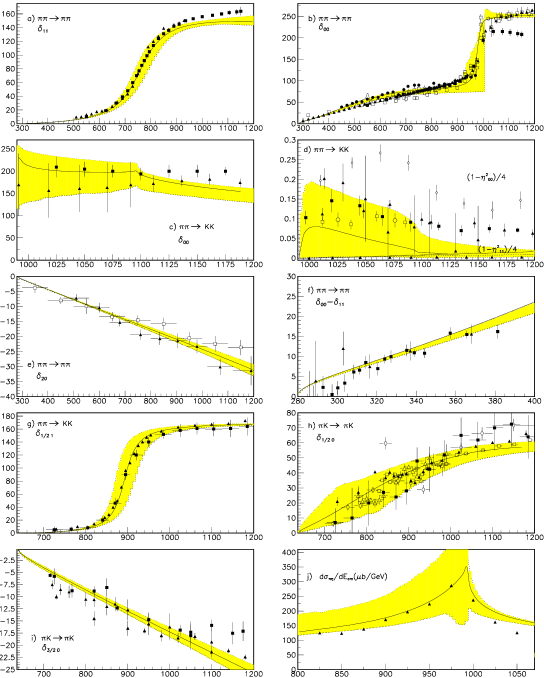
Figure 1: IAM fit to meson-meson scattering data, set II in Table 1. The uncertainties cover the estimated systematic errors. The statistical errors from the fit would be much smaller. The data comes from pipidata

Threshold	Experiment	IAM fit I	ChPT ${O}(p^{4})\hskip 14.22636pt$	ChPT ${O}(p^{6})$
parameter		GomezNicola:2001as	Dobado:1996ps ; Kpi	Amoros:2000mc
$a_{0\,0}$	0.26 $\pm$0.05	0.231${}^{+0.003}_{-0.006}$	0.20	0.219$\pm$0.005
$b_{0\,0}$	0.25 $\pm$0.03	0.30$\pm$ 0.01	0.26	0.279$\pm$0.011
$a_{2\,0}$	-0.028$\pm$0.012	-0.0411${}^{+0.0009}_{-0.001}$	-0.042	-0.042$\pm$0.01
$b_{2\,0}$	-0.082$\pm$0.008	-0.074$\pm$0.001	-0.070	-0.0756$\pm$0.0021
$a_{1\,1}$	0.038$\pm$0.002	0.0377$\pm$0.0007	0.037	0.0378$\pm$0.0021
$a_{1/2\,0}$	0.13…0.24	0.11${}^{+0.06}_{-0.09}$	0.17
$a_{3/2\,0}$	-0.13…-0.05	-0.049${}^{+0.002}_{-0.003}$	-0.5
$a_{1/2\,1}$	0.017…0.018	0.016$\pm$0.002	0.014
$a_{1\,0}$		0.15${}^{+0.07}_{-0.11}$	0.0072

Table 2: Scattering lengths $a_{I\,J}$ and slope parameters $b_{I\,J}$ for different meson-meson scattering channels. For experimental references see GomezNicola:2001as . Let us remark that our one-loop IAM results at threshold are very similar to those of two-loop ChPT.

To conclude, we show in Table 2 the values of the scattering lengths and slopes, which confirms that we have a simultaneous description of the low energy and resonant regions of meson-meson scattering. As we have seen in Table 1, all this is achieved with chiral parameters compatible with those from standard ChPT. Hence, since the expressions are fully renormalized, we are not including any dependence on any spurious parameter.

Another result of relevance in the context of unitarized ChPT has been the consideration of higher order effects. There is indeed a simple way to extend the IAM to higher orders, already proposed in Dobado:1996ps , and first applied to two loop $\pi\pi$ scattering and the pion form factor Hannah:1997ux , also obtaining remarkable results. This study has been very recently extended in Nieves:2001de with a careful analysis of the uncertainties. This amplitude depends on the $O(p^{4})$ and $O(p^{6})$ parameters through six combinations only, called $b_{i}$. Despite the poor knowledge about these two-loop parameters, listed in Table 3, in Nieves:2001de a good description of the data is found, including the $\sigma$ and $\rho$ regions, with parameters, again given in Table 3, compatible within errors with those already in the literature. The error analysis carried out in Nieves:2001de is also of relevance because unitarization methods in general, and the IAM in particular, are mainly criticized for their violation of crossing symmetry. However, in that work it was shown that the IAM crossing violations, “quantified in terms of Roskies sum rules” , and taking into account the present experimental uncertainties are “ not very large in percentage terms”.

We finish this section about the unitarized description of meson-meson scattering reviewing the recent generalization of the IAM Dobado:2001rv to channels where the leading order, $T_{2}$, vanishes. For instance, that is the case for all channels with $J>1$, so that eq.(5) cannot be applied. Note also that eq.(3) implies that the perturbative imaginary part vanishes up to $O(p^{8})$. However, despite these difficulties, and using again a dispersive approach, it has been possible to generalize the IAM and unitarize the $(2,0)$ channel, using:

$$t^{IAM}=\frac{t_{4}}{1-t_{6}/t_{4}-t_{8}/t_{4}+t_{6}^{2}/t_{4}^{4}}.$$ (6)

Up to the moment not even the $O(p^{8})$ $SU(2)$ pion ChPT Lagrangian is known. Hence, we have used the two-loop $SU(2)$ calculation and we have estimated the $O(p^{8})$ contribution to $\pi\pi$ scattering in the chiral limit, since, as it is the only term surviving in the $m_{\pi}\rightarrow 0$ limit, we expect it to dominate at the energies $\sqrt{s}>>m_{\pi}$ where the first $f_{2}(1250)$ resonance appears. In this way we are only introducing an additional parameter, whose size, on dimensional grounds, should be $c\simeq(1/4\pi f_{0})^{8}\simeq 3\times 10^{-25}\hbox{MeV}^{-8}$

	$10^{2}b_{1}$	$10^{2}b_{2}$	$10^{3}b_{3}$	$10^{3}b_{4}$	$10^{4}b_{5}$	$10^{4}b_{6}$
$O(p^{6})$ ChPT bijnens	-9.2 … -8.6	8.0 … 8.9	-4.3 … -2.6	4.8 … 7.1	-0.4 … 2.3	0.7 … 1.5
$O(p^{6})$ IAM Nieves:2001de	$-7.7\pm 1.3$	$7.3\pm 0.7$	$-1.8\pm 1.6$	$4.8\pm 0.1$	$1.3\pm 0.2$	$0.2\pm 0.2$
set I	-3	4	3.8	7	8.7	1.6
set II	-6.6	6.4	-3.6	6.7	4.0	1.5

Table 3: Estimates of the $O(p^{6})$ parameters are given in row two. In the third row we give values that, with the IAM up to $O(p^{6})$, fit very well $\pi\pi$ scattering in the $(I,J)=(0,0),(1,1)$ and $(2,0)$ channels. Set I with eq.(8) describes remarkably well the $I=0,J=2$ data, but only agrees in the order of magnitude with previous values. Set II is closer to Nieves:2001de , but yields a narrower resonance (see Fig.2.a), due to other coupled states not present in our approach.

Thus, in Fig.2.a (dashed line) we compare the $(I,J)=(0,2)$ phase shift data with the results of applying eq.(6) to the ChPT amplitude just described, using the set I of parameters given in Table 3. By fitting, it is possible to force a remarkable description of the experiment, including the $f_{2}(1250)$ resonance. However that is not realistic since the $f_{2}(1250)$ has an $85\%$ decay to $\pi\pi$ and should not be described with $\pi\pi$ scattering only. For that reason the set I, although with the correct order of magnitude, does not compare well with the values given in the literature, listed in column two and three of Table 3. For illustrative purposes, we also show, as a dotted line, the result using set II in Table 3, which is obtained if we allow for a $15\%$ narrower resonance. That is not a fit, but the parameters are much closer to those given in the literature. Finally, we want to remark that for any set of parameters that we have found yielding results like those in Fig.2.a, the values needed for the $c$ constant lie in the $c\simeq 10^{-25}$ to $10^{-24}\,$ MeV^-8 range, consistently with our expectations.

We have therefore checked that the IAM produces good results as soon as we provide it with reasonable inputs, also in channels with higher angular momenta.

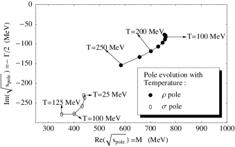
Figure 2: a) The $,I=0,J=2$ $\pi\pi$ scattering phase shift pipidata and the results of our unitarized chiral resonance model (continuous line), of eq.(6) with the parameters in set I (dashed line), and with those in set II (dotted line) in Table 3. b) Thermal evolution of the $\sigma$ and $\rho$ poles.

3 IV. Poles associated to resonances

In this section we will investigate whether the unitarized complete meson-meson amplitudes obtain the same poles as obtained with previous approaches. This is of relevance since, for instance, both the $\sigma$ and $\kappa$ scalar states are rather controversial even though their poles have been found by several other groups using different techniques newsigma ; JA . The debate has become increasingly interesting when recent experiments seem to require such poles charm to describe completely different processes.

The most interesting features of the chiral unitary approaches is that the poles thus generated are not included in the original ChPT Lagrangian and hence appear without any theoretical prejudice toward their existence, classification in multiplets, or nature. Of particular interest for this workshop is the simultaneous generation of the scalar resonances $\sigma,\kappa,a_{0}(980)$ and $f_{0}(980)$ in a chiral context, so that it seems very natural to interpret them as a nonet. Nevertheless, we should distinguish two different resonance generation mechanisms: already in Oller:1997ti it was noted that to generate the scalars just the leading order and a cutoff was enough, whereas the vector mesons require the chiral parameters, particularly $L_{1},L_{2}$ and $L_{3}$ Oller:1997ng . Of course, the chiral parameters are always present , but it seems that their values are not related to the hypothesized light scalar nonet. Since the vectors are fairly well established $q\bar{q}$ states, this difference suggests that scalars like the $\sigma$, $\kappa$, etc may have a different nature. With the amplitudes described in the previous sections we expect to reach a more conclusive statement, since they respect the chiral expansion, and, being completely renormalized, have no spurious dependence on any cutoff or dimensional regularization scale. In addition, the fact that we use chiral parameters compatible with previous determinations ensures that our description is consistent with other low energy processes.

Thus, in Table 4 we show the pole position for the resonances, including uncertainties, for the different IAM parameter sets given in Table 1. For comparison we provide in the first row those obtained in the “approximated” IAM Oller:1997ng , whereas we list in Table 5 the poles listed presently in the PDG PDG . These results deserve some comments:

• The vectors $\rho(770)$ and $K^{*}(892)$, are very stable within chiral unitary approaches. Their positions are almost the same irrespective of whether one uses the single channel Truong:1988zp ; Dobado:1996ps , the approximated coupled channel Oller:1997ng or the complete IAM GomezNicola:2001as .

• The $\sigma$ and $\kappa$ pole positions are robust within these approaches. No matter what version of the IAM is used. Note the small uncertainties in some of their parameters, in very good agreement with recent experiments charm .

• The $f_{0}(980)$ has a sizable decay to two different channels and therefore it can only be studied in a coupled channel formalism. In practice, both the approximated and complete IAM generate a pole associated to this state at approximately the same mass. However, as already remarked the unitarized ChPT amplitudes using just $f_{\pi}$ GomezNicola:2001as , yield a too narrow width. The good news is that it can be well accommodated using $f_{\pi}$, $f_{K}$ and $f_{\eta}$ Coimbra .

• The $a_{0}(980)$ also requires a coupled channel formalism, and the data on this region is well described either by the approximated or the complete IAM. However, the presence of a pole is strongly dependent on whether we write the ChPT amplitudes only in terms of $f_{\pi}$, or using the three $f_{\pi}$, $f_{K}$ and $f_{\eta}$. In the first case, as already pointed out in Uehara:2002nv , the use of the “approximated” IAM with just $f_{\pi}$, favored a “cusp” interpretation of the $a_{0}(980)$ enhancement in $\pi\eta$ production. With the complete IAM we do not find a pole near the $a_{0}(980)$ enhancement and indeed the $\pi\eta$ phase-shift does not cross $\pi/2$ and it neither has a fast phase movement. In contrast, when expressing $f_{0}$ in terms of $f_{\pi}$, $f_{K}$ and $f_{\eta}$ as described in the previous section, we do find a pole and its associated fast phase movement through $\pi/2$, either with the approximated or complete IAM. Thus, this pole is rather unstable as can be noticed from its large uncertainties in Table 4. We are somewhat more favorable toward the second interpretation because it is also able to describe better the $f_{0}(980)$ width. But the two possibilities remain open.

$\sqrt{s_{pole}}$(MeV)	$\rho$	$K^{*}$	$\sigma$	$f_{0}$	$a_{0}$	$\kappa$
${}^{\hbox{IAM Approx}}_{\;\;\;\hbox{(no errors)}}$	759-i 71	892-i 21	442-i 227	994-i 14	1055-i 21	770-i 250
IAM I	760-i 82	886-i 21	443-i 217	988-i 4	cusp?	750-i 226
(errors)	$\pm$ 52$\pm$ i 25	$\pm$ 50$\pm$ i 8	$\pm$ 17$\pm$ i 12	$\pm$ 19$\pm$ i 3		$\pm$18$\pm$i 11
IAM II	754-i 74	889-i 24	440-i 212	973-i 11	1117-i 12	753-i 235
(errors)	$\pm$ 18$\pm$ i 10	$\pm$ 13$\pm$ i 4	$\pm$ 8$\pm$ i 15	${}^{+39}_{-127}$ ${}^{+i\,189}_{-i\,11}$	${}^{+24}_{-320}$ ${}^{+i\,43}_{-i\,12}$	$\pm$ 52$\pm$ i 33
IAM III	748-i68	889-i23	440-i216	972-i8	1091-i52	754-i230
(errors)	$\pm$ 31$\pm$ i 29	$\pm$ 22$\pm$ i 8	$\pm$ 7$\pm$ i 18	${}^{+21}_{-56}$$\pm$ i 7	${}^{+19}_{-45}$ ${}^{+i\,21}_{-i\,40}$	$\pm$ 22$\pm$ i 27

Table 4: Pole positions (with errors) in meson-meson scattering. When close to the real axis the mass and width of the associated resonance is $\sqrt{s_{pole}}\simeq M-i\Gamma/2$.

PDG2002	$\rho(770)$	$K^{*}(892)^{\pm}$	$\sigma$ or $f_{0}(600)$	$f_{0}(980)$	$a_{0}(980)$	$\kappa$
Mass (MeV)	$771\pm 0.7$	$891.66\pm 0.26$	(400-1200)-i (300-500)	$980\pm 10$	$980\pm 10$	not
Width (MeV)	$149\pm 0.9$	$50.8\pm 0.9$	(we list the pole)	40-100	50-100	listed

Table 5: Mass and widths or pole positions of the light resonances quoted in the PDG PDG . Recall that for narrow resonances $\sqrt{s_{pole}}\simeq M-i\Gamma/2$

Let us remark that the $f_{0}(980)$ and $a_{0}(980)$ resonances are very close to the $K\bar{K}$ threshold, which can induce a considerable distortion in the resonance shape, whose relation to the pole position could be far from that expected for narrow resonances. In addition these states have a large mass and it is likely that their nature should be understood from a mixture with heavier states.

4 IV. Thermal evolution of the $\sigma$ and $\rho$ mesons.

In a recent paper we have calculated the temperature one-loop corrections to the $\pi\pi$ scattering amplitude GomezNicola:2002tn . These corrections are finite although they appear through the pion loops and consequently, do not include any additional parameter in the expression of the amplitude. A discussion on the rigorous meaning of such an amplitude in terms of Thermal Field Theory, as well as the explicit expression of the thermal corrections can be found in GomezNicola:2002tn . For our purposes here, it is enough to say that the thermal amplitude can be projected into partial waves that satisfy a generalized perturbative unitary relation:

$${\mbox{Im}\,}t_{2}(s)=0,\qquad{\mbox{Im}\,}t_{4}(s;\beta)=\sigma_{T}(S_{0})\left|t_{2}(s)\right|^{2}\ ,\quad S_{0}>2m_{\pi},\beta=1/T$$ (7)

where

$$\sigma_{T}(E)=\sigma(E^{2})\left[1+\frac{2}{\exp({\beta|E|/2})-1}\right]$$ (8)

is the thermal two-particle phase space in the c.o.m. frame. It is nothing but the phase space $\sigma(s)$ defined above but corrected by the presence of two-pion states following a Bose-Einstein distribution.

In the dilute gas approximation it is natural to assume that this unitarity relation should be satisfied to all order, which thus leads to a straightforward thermal generalization of the IAM Dobado:2002xf . In the elastic approximation it is again the IAM formula, but simply using the thermal amplitudes,i.e., replacing $t_{4}(s)$ by $t_{4}(s,\beta)$, calculated in GomezNicola:2002tn . Obviously, we recover the zero temperature unitarized amplitude when we make $T\rightarrow 0$. We recall again that the temperature dependence appears at this order through finite contributions to the loop functions, but not in the chiral parameters. Thus, once we have parameters that generate the $\sigma$ and $\rho$ at $T=0$, we can follow their thermal evolution by changing $T$. Nevertheless, although the unitarization allows to extend the ChPT applicability range, the dilute approximation implies that we can only look at temperatures up to $T\simeq 200\,\hbox{MeV}$. Thus, in Fig2.b Dobado:2002xf we can see the thermal evolution of the $\sigma$ and $\rho$ poles. Note that the width of both resonances is growing with the temperature. For the $\rho$ this is in good agreement with observations of the dilepton spectra produced in Heavy Ion Collisions. For the $\sigma$ it could be interpreted as a signal of chiral symmetry restoration.

5 V. Unitarized ChPT and the large $N_{c}$

QCD is not perturbative below 1 or 2 GeV. However, to understand many qualitative features of QCD and also as a guiding line to organize calculations we can use the large $N_{c}$ expansion largen , even though the number of colors is actually $N_{c}=3$. The advantage of the large $N_{c}$ limit to study resonances is that $q\bar{q}$ states become bound states as $N_{c}\rightarrow\infty$. More quantitatively, their mass should remain almost constant $M\simeq O(1)$, whereas their decay width to two mesons should behave as $\Gamma\simeq O(1/N_{c})$. A similar behavior holds for glueballs decaying to two mesons. In contrast, some multiquark states as $qq\bar{q}\bar{q}$ are expected to become unbound, i.e., to be part of the meson-meson continuum Jaffe .

The parameters in the ChPT Lagrangian inherit the large $N_{c}$ dynamics of QCD. In particular, the meson masses and decay constants behave as $f_{\pi},f_{K},f_{\eta}=O(\sqrt{N_{c}})$ and $M_{\pi},M_{K},M_{\eta}=O(1)$. In Table 6, we list the large $N_{c}$ behavior of the chiral parameters chptlargen , which is established in a model independent way. Note however that there is an uncertainty on the renormalization scale that corresponds to $N_{c}=3$, although generically it should lie in the $\mu\simeq 0.5-1\,$GeV range.

Parameter $\times 10^{-3}$	ChPT $\mu=770$ MeV	IAM I $\mu=770$ MeV	Large $N_{c}$ behavior
$2L_{1}-L_{2}$	$-0.6\pm 0.2$	$0.56\pm 0.10$	$O(1)$
$L_{2}$	$1.35\pm 0.3$	$1.21\pm 0.10$	$O(N_{c})$
$L_{3}$	$-3.5\pm 1.1$	$-2.79\pm 0.14$	$O(N_{c})$
$L_{4}$	$-0.3\pm 0.5$	$-0.36\pm 0.17$	$O(1)$
$L_{5}$	$1.4\pm 0.5$	$1.4\pm 0.5$	$O(N_{c})$
$L_{6}$	$-0.2\pm 0.3$	$0.07\pm 0.08$	$O(1)$
$L_{7}$	$-0.4\pm 0.2$	$-0.44\pm 0.15$	$O(1)$
$L_{8}$	$0.9\pm 0.3$	$0.78\pm 0.18$	$O(N_{c})$

Table 6: Different sets of chiral parameters ($\times 10^{3}$). For illustration, the ChPT and IAM I columns are repeated from Table 1. Other IAM sets give similar results. The last column shows the leading large $N_{c}$ behavior, calculated from QCD.

Since we have built our unitarized amplitudes using the completely renormalized ChPT expressions, we can now study the large $N_{c}$ behavior of the generated resonances and get a hint on their nature. We will simply scale the ChPT parameters at $\mu=770\,$MeV in the IAM amplitudes fitted to the data, which therefore correspond to $N_{c}=3$. As already commented, for narrow resonances the pole position $\sqrt{s_{pole}}\simeq M-i\Gamma/2$ $M$ and $\Gamma$ being the mass and width of the resonance. From the spectroscopic point of view, a resonance could be a mixture of several states, but comparing its large $N_{c}$ behavior we could, in principle, elucidate the nature of the dominant component. Indeed, already in JA it was shown, using unitarized meson-meson scattering from a chiral resonance Lagrangian and only the s-loops unitarized with an N/D method, that the lightest scalar resonances did not behave as one would expect for $\bar{q}q$ states. We will next show the results of our, still preliminary, study with the unitarized ChPT renormalized amplitudes. Of course, if most of the states of the mixture disappears in the large $N_{c}$ limit, a very small portion of a $q\bar{q}$ could become more patent if we increase $N_{c}$ sufficiently. To avoid these effects we will present results for $N_{c}$ up to about 20.

Figure 3: Large $N_{c}$ dependence of the pole positions in the lower half of the second Riemann $\sqrt{s}$ sheet of the meson meson scattering amplitude, obtained from the unitarized one-loop Chiral Perturbation Theory calculation. For each value of $N_{c}$ the pole is represented by a dot, in different meson-meson scattering channel. Note that the $\sigma$ and $\kappa$ behavior is opposite to that of well know vector states as the $\rho$ and $K^{*}$.

Thus, Fig.3 shows the large $N_{c}$ behavior of the poles in several channels of meson meson scattering. Each dot corresponds to a different value of $N_{c}$. First of all, we want to be sure that the method works for well established $q\bar{q}$ states and so we turn to vector resonances. Hence, on the top left, we represent the movement of the $\rho(770)$ pole the $I,J=1,1$ channel of $\pi\pi$ scattering. On the top right we display the $K^{*}(982)$ movement in the $I,J=1,1/2$ channel of $\pi K$ scattering. Remarkably, the IAM reproduces the expected $q\bar{q}$ behavior since the mass of both vectors tends to a constant and their width decreases as $1/N_{c}$. If we did not know it already, this would be a strong hint that both states are indeed $q\bar{q}$ states. Let us remark that ChPT is built in terms of mesons, not of quarks, but the QCD large $N_{c}$ dynamics is correctly inherited in the $L_{i}$ values.

Let us then turn to the controversial scalar resonances, subject of this workshop.. On the bottom left of Fig.3 we represent the movement of the pole commonly associated to the $\sigma$ and, on the right, that associated with the $\kappa$. Note that we keep the notation $\sqrt{s_{pole}}\simeq M-i\Gamma/2$, although these poles are so far from the real axis (so wide) that the interpretation in terms of mass and width is no longer straightforward. However, it is very clear that their behavior is completely at variance with that expected for $q\bar{q}$ states. We can see that in both cases, either $M$ or $\Gamma$grow as $N_{c}$ is increased. This behavior does not correspond to a $q\bar{q}$ or glueball nature. Other interpretations should be invoked, although we want to remark that the one that is becoming more widely accepted, namely, the four-quark state interpretation Jaffe (and also the two-meson molecules), is able to accommodate the fact that these states become the meson-meson continuum as $N_{c}$ grows.

6 Conclusion and outlook

In this talk I have reviewed the most recent developments in the unitarization of the Chiral Perturbation Theory amplitudes, paying particular attention to the Inverse Amplitude Method. The outcome of this approach is of interest for meson spectroscopy since it can generate resonances, without including them in the ChPT Lagrangian, and respecting simultaneously chiral symmetry and unitarity.

I have reviewed how unitarized meson-meson scattering ChPT amplitudes provide a simultaneous description of the low energy and resonant regions below 1.2 GeV, generating the poles associated to the $\rho,K^{*},\sigma,\kappa,a_{0}$ and $f_{0}$ states. This description respects the low energy chiral expansion up to next to leading order and the unitarized fit leads to parameters compatible with those of standard ChPT. Remarkably, it yields scattering lengths compatible with higher order calculations and the most recent low energy data. The amplitudes are completely renormalized and scale independent, thus avoiding any spurious dependence from artificial scales. We have also seen that some of the drawbacks, as crossing symmetry, seem to be well under control, given the present experimental uncertainties. The IAM is very simple to implement, and it can be systematically extended to higher orders. The few unitarized calculation to two loops indeed provide good descriptions of $\pi\pi$ scattering again with compatible parameters. It has also been recently extended to channels with vanishing leading order providing a satisfactory description of the $f_{2}(1250)$ resonance. The description in terms of poles is robust, with the possible exception of the $a_{0}$ (that could alternatively be interpreted as a cusp), and these states seem to be an unavoidable requirement of chiral symmetry and unitarity.

We have also shown how it can be generalized to thermal amplitudes, which allowed us to study the temperature evolution of the $\sigma$ and $\rho$ resonances.

Concerning the nature of these states, we have presented a preliminary study of the large $N_{c}$ behavior of the poles. We have seen that the vectors generated with the IAM follow remarkably well the expected $q\bar{q}$ behavior. In contrast, the $\sigma$ and $\kappa$ states, behave in a completely different way, ruling out a $q\bar{q}$ or glueball interpretation. A $qq\bar{q}\bar{q}$ interpretation seems at least qualitatively adequate large $N_{c}$ evolution.

The large $N_{c}$ study is still preliminary and we are finishing the analysis of the $f_{0}$ and $a_{0}$ behavior, which have larger uncertainties and a complicated interpretation due to the proximity of thresholds and possible mixings with more massive multiplets . We are also estimating the errors due to the uncertainty in the renormalization scale where the large $N_{c}$ scaling is imposed. Finally, we are presently looking directly at the large $N_{c}$ to avoid using poles whose interpretation for wide resonances is delicate. Work is still in progress in all these directions.

References

- (1) S. Weinberg, Physica A96 (1979) 327. J. Gasser and H. Leutwyler, Annals Phys. 158 (1984) 142.
- (2) J. Gasser and H. Leutwyler, Nucl. Phys. B 250 (1985) 465.
- (3) A. A. Andrianov, Phys. Lett. B 157, 425 (1985). A. A. Andrianov and L. Bonora, Nucl. Phys. B 233, 232 (1984). D. Espriu, E. de Rafael and J. Taron, Nucl. Phys. B 345 (1990) 22 [Erratum-ibid. B 355 (1991) 278]. S. Peris and E. de Rafael, Phys. Lett. B 348 (1995) 539
- (4) G. Ecker, J. Gasser, A. Pich and E. de Rafael, Nucl. Phys. B 321, 311 (1989).
- (5) T. N. Truong, Phys. Rev. Lett. 61 (1988) 2526. Phys. Rev. Lett. 67, (1991) 2260; A. Dobado, M.J.Herrero and T.N. Truong, Phys. Lett. B235 (1990) 134. A. Dobado and J. R. Pelaez, Phys. Rev. D 47 (1993) 4883.
- (6) A. Dobado and J. R. Pelaez, Phys. Rev. D 56 (1997) 3057.
- (7) J. Nieves and E. Ruiz Arriola, Nucl. Phys. A 679 (2000) 57
- (8) J. A. Oller, E. Oset and J. R. Peláez, Phys. Rev. Lett. 80 (1998) 3452; Phys. Rev. D 59 (1999) 074001 [Erratum-ibid. D 60 (1999) 099906]. Phys. Rev. D 62 (2000) 114017.
- (9) F. Guerrero and J. A. Oller, Nucl. Phys. B 537 (1999) 459 [Erratum-ibid. B 602 (2001) 641].
- (10) A. Gómez Nicola and J. R. Peláez, Phys. Rev. D 65 (2002) 054009
- (11) J. R. Pelaez and A. Gomez Nicola, AIP Conf. Proc. 660 (2003) 102 [arXiv:hep-ph/0301049].
- (12) V. Bernard, N. Kaiser, U.G. Meissner, Phys. Rev. D43 (1991) 2757; Nucl. Phys. B357 (1991) 129; Phys. Rev. D44 (1991) 3698.
- (13) G. Amorós, J. Bijnens and P. Talavera, Nucl. Phys. B602 (2001) 87.
- (14) J. Bijnens, G. Colangelo and J. Gasser, Nucl. Phys. B427 (1994) 427.
- (15) G. Amoros, J. Bijnens and P. Talavera, Nucl. Phys. B 585 (2000) 293 [Erratum-ibid. B 598 (2001) 665].
- (16) S. D. Protopopescu et al., Phys. Rev. D7, (1973) 1279; P. Estabrooks and A.D.Martin, Nucl.Phys.B79, (1974) 301. G. Grayer et al., Nucl. Phys. B75, (1974) 189. D. Cohen, Phys. Rev. D22, (1980) 2595. W. Hoogland et al., Nucl. Phys. B126 (1977) 109. M. J. Losty et al., Nucl. Phys. B69 (1974) 185. R. Mercer et al., Nucl. Phys. B32 (1971) 381. P. Estabrooks et al., Nucl. Phys. B133 (1978) 490. H. H. Bingham et al., Nucl. Phys. B41 (1972) 1. S. L. Baker et al., Nucl. Phys. B99 (1975) 211. D. Aston et al. Nucl. Phys. B296 (1988) 493. D. Linglin et al., Nucl. Phys. B57 (1973) 64 .S. Pislak et al. [BNL-E865 Collaboration], Phys. Rev. Lett. 87 (2001) 221801. P. Estabrooks and A.D. Martin, Nucl. Phys. B79 (1974) 301 C.D. Froggat and J.L. Petersen, Nucl. Phys. B129(1977)89.
- (17) T. Hannah, Phys. Rev. D 55 (1997) 5613
- (18) J. Nieves, M. Pavon Valderrama and E. Ruiz Arriola, Phys. Rev. D 65 (2002) 036002
- (19) J. Bijnens et al., Phys. Lett. B374 (1996) 210; Nucl. Phys. B508 (1997) 263.
- (20) A. Dobado and J. R. Pelaez, Phys. Rev. D 65 (2002) 077502 [arXiv:hep-ph/0111140].
- (21) R.L. Jaffe, Phys. Rev. D15 267 (1977); Phys. Rev. D15, 281 (1977). E. van Beveren et al. Z. Phys. C30, 615 (1986). R. Kaminski, L. Lesniak and J. P. Maillet, Phys. Rev. D 50 (1994) 3145. M. Harada, F. Sannino and J. Schechter, Phys. Rev. D 54 (1996) 1991 R. Delbourgo and M. D. Scadron, Mod. Phys. Lett. A 10 (1995) 251. S. Ishida et al., Prog. Theor. Phys. 95 (1996) 745. N. A. Tornqvist and M. Roos, Phys. Rev. Lett. 76 (1996) 1575. S. Ishida et al, Prog. Theor. Phys. 98,621 (1997). D. Black, A. H. Fariborz, F. Sannino, J. Schechter. Phys. Rev. D58:054012,1998. E. van Beveren and G. Rupp, Eur. Phys. J. C 22 (2001) 493 E. van Beveren and G. Rupp, arXiv:hep-ph/0201006.
- (22) J. A. Oller and E. Oset, Phys. Rev. D 60 (1999) 074023
- (23) E791 Collaboration, Phys. Rev. Lett. 86,(2001) 770. E. M. Aitala et al. [E791 Collaboration], Phys. Rev. Lett. 89 (2002) 121801 C. Gobel for the E791 Collab. hep-ex/0012009.
- (24) J. A. Oller and E. Oset, Nucl. Phys. A 620 (1997) 438 [Erratum-ibid. A 652 (1999) 407]
- (25) K. Hagiwara et al., Phys. Rev. D 66, 010001 (2002).
- (26) M. Uehara, arXiv:hep-ph/0204020.
- (27) A. Gomez Nicola, F. J. Llanes-Estrada and J. R. Pelaez, Phys. Lett. B 550 (2002) 55
- (28) A. Dobado, A. Gomez Nicola, F. J. Llanes-Estrada and J. R. Pelaez, Phys. Rev. C 66 (2002) 055201
- (29) G. ’t Hooft, Nucl. Phys. B 72 (1974) 461. C. Rosenzweig, J. Schechter and C. G. Trahern, Phys. Rev. D 21 (1980) 3388. E. Witten, Annals Phys. 128 (1980) 363.
- (30) R. L. Jaffe, Proceedings of the Intl. Symposium on Lepton and Photon Interactions at High Energies. Physikalisches Institut, University of Bonn (1981) . ISBN: 3-9800625-0-3
- (31) V. Cirigliano, G. Ecker, H. Neufeld and A. Pich, arXiv:hep-ph/0305311.