Abstract

The scalar sector of the linear formulation of the degenerate BESS model is analyzed. The model predicts two additional scalar states which mix with the SM Higgs. As a consequence the properties of the SM Higgs are modified and Higgs precision measurements can constrain the mixing angle. One of the two additional Higgses has no coupling to fermions and suppressed couplings to ordinary gauge bosons, therefore its detection is difficult. The production of the other two Higgses at future $e^{+}e^{-}$ linear colliders in the Higgstrahlung and fusion channels is investigated.

  PACS: 12.60.-i,12.60.Cn,12.60.Fr
Keywords: extended gauge symmetries, extended Higgs sector, strong symmetry breaking.

1 Introduction

There has been recently a renewed interest in models with extended electroweak symmetry in the context of little Higgs models (for a review see [1]). Their low energy description is based on effective lagrangians constructed using extended gauge symmetries including, in general, copies of $SU(2)$ and $U(1)$ groups. Similar gauge symmetry structures also appear in effective lagrangians for technicolor and non commuting extended technicolor [2]. The degenerate BESS model [3] is a non linear description based on the gauge symmetry group ${\cal G}=SU(2)_{L}\otimes U(1)_{Y}\otimes SU(2)^{\prime}_{L}\otimes SU(2)^{\prime}_{R}$ and therefore can be used as a general parameterization of classes of models. New vector gauge bosons are introduced and, in order to include the possible (composite) scalar fields, a linear formulation was proposed [4], describing the breaking of the group $\cal G$ at some high energy scale $u$ to $SU(2)_{weak}\otimes U(1)$ and finally, at the electroweak scale $v$, to $U(1)_{em}$. The model, in the limit of large $u$, gives back the Standard Model (SM) with a light Higgs and the contributions to the $\epsilon$ (or $S,T,U$) parameters are $O((v/u)^{2}s_{\varphi}^{2})$, being $\varphi$ the mixing angle of the charged gauge boson sector. As a consequence the model is only weakly constrained by the electroweak precision measurements. The phenomenology of the additional gauge vector bosons has been already addressed: detection of new vector resonances will be possible at the LHC up to masses of approximately 2 TeV for $s_{\varphi}\sim 0.14$ [5]. Aim of this paper is to perform the analysis of the scalar sector of the model and study its properties at future linear colliders (LC’s) which offer the possibility of detecting the Higgs and also performing precision measurements of Higgs boson cross sections, partial widths and of the trilinear Higgs coupling. The investigation of the scalar sector at the LHC will be the subject of a separate paper.

In Section 2 we review the scalar sector of the linear degenerate BESS model and derive the couplings of the scalars to fermions, gauge bosons and their self-interactions. In Sections 3 and 4 analytical and numerical results are obtained for the widths of the Higgses and the production cross sections at future LC’s. In Section 5 we study the bounds on the parameters of the scalar sector of the model from the LC measurements.

2 The Linear BESS model: a new parameterization

Existing experimental data confirm with great accuracy the SM of the electroweak interactions, therefore only extensions which smoothly modify its predictions are still conceivable. There are examples of strong symmetry breaking schemes, like degenerate BESS [3], satisfying this property. The model describes, besides the standard $W^{\pm}$, $Z$ and $\gamma$ vector bosons, two new triplets of spin 1 particles, $V_{L}$ and $V_{R}$. The interest in this scheme was due to its decoupling property: in the limit of infinite mass of the heavy vector bosons one gets back the Higgsless SM. The original philosophy of the non-linear version was based on the idea that the non-linear realization would be the low-energy description of some underlying dynamics giving rise to the breaking of the electroweak symmetry. A linear realization of this model (L-BESS) was proposed in [4]. This scenario is a possible effective description of technicolor and of its generalizations as non-commuting technicolor models [2], where an underlying strong dynamics produces heavy Higgs composite particles. The L-BESS model describes the theory, as a renormalizable theory, at the level of its composite states, vectors (the new heavy bosons), and scalars (Higgs bosons).

Let us first review the main properties of the L-BESS model, in particular of its scalar sector, on which we will focus in the present study. The model is a $SU(2)_{L}\otimes U(1)_{Y}\otimes SU(2)_{L}^{\prime}\otimes SU(2)_{R}^{\prime}$ gauge theory, breaking at some high scale $u$ to $SU(2)_{weak}\otimes U(1)$ and breaking again at the electroweak scale $v$ to $U(1)_{em}$.

The L-BESS model contains, besides the standard Higgs sector described by the field $\tilde{U}$, two additional scalar fields $\tilde{L}$ and $\tilde{R}$. They belong to the (2,2,0,0), (2,0,2,0) and (0,2,0,2) representations of the global symmetry group $G=SU(2)_{L}\otimes SU(2)_{R}\otimes SU(2)_{L}^{\prime}\otimes SU(2)_{R}^{\prime}$, respectively. The two breakings are induced by the vacuum expectation values $\langle\tilde{L}\rangle=\langle\tilde{R}\rangle=u$ and $\langle\tilde{U}\rangle=v$. We will assume $u\gg v$. Proceeding in the standard way, we build up the kinetic terms for the fields in terms of the covariant derivatives with respect to the local $SU(2)_{L}\otimes U(1)_{Y}\otimes SU(2)_{L}^{\prime}\otimes SU(2)_{R}^{\prime}$, by introducing ${\vec{V}}_{L}~{}({\vec{V}}_{R})$ as gauge fields of $SU(2)_{L}^{\prime}~{}(SU(2)_{R}^{\prime})$, with a common gauge coupling $g_{2}$, whereas $g_{0}$ and $g_{1}$ are the gauge couplings of the $SU(2)_{L}$ and $U(1)_{Y}$ gauge groups respectively. The scalar potential responsible for the breaking of the original symmetry down to the $U(1)_{em}$ group is constructed by requiring invariance with respect to the group $G$ and the discrete symmetry ${\tilde{L}}\leftrightarrow{\tilde{R}}$. As far as the fermions are concerned they transform as in the SM with respect to the group $SU(2)_{L}\otimes U(1)_{Y}$, correspondingly the Yukawa terms are built up exactly as in the SM [3].

We parameterize the scalar fields as $\tilde{L}=\tilde{\rho}_{L}L$, $\tilde{R}=\tilde{\rho}_{R}R$, $\tilde{U}=\tilde{\rho}_{U}U$, with ${L}^{\dagger}{L}=I$, ${R}^{\dagger}{R}=I$ and ${U}^{\dagger}{U}=I$. The scalar potential is expressed in terms of three Higgs fields:

$$V(\tilde{\rho}_{U},\tilde{\rho}_{L},\tilde{\rho}_{R})=2\mu^{2}(\tilde{\rho}_{L}^{2}+\tilde{\rho}_{R}^{2})+\lambda(\tilde{\rho}_{L}^{4}+\tilde{\rho}_{R}^{4})+2m^{2}\tilde{\rho}_{U}^{2}+h\tilde{\rho}_{U}^{4}+2f_{3}\tilde{\rho}_{L}^{2}\tilde{\rho}_{R}^{2}+2f\tilde{\rho}_{U}^{2}(\tilde{\rho}_{L}^{2}+\tilde{\rho}_{R}^{2}).$$ (1)

We assume $m^{2},\mu^{2}<0$, and $\lambda,h>0$ for the vacuum stability.

From the stationarity conditions, the requirements $\mu^{2}<0$ and $m^{2}<0$ lead to:

$$(f_{3}+\lambda)+fx^{2}>0\,,~{}~{}~{}~{}~{}~{}~{}hx^{2}+2f>0\,~{}~{}~{}~{}~{}{\rm with}~{}~{}~{}~{}~{}x=v/u.$$ (2)

After shifting the fields by their v.e.v’s $u,v\neq 0$, the mass eigenvalues are:

$$m_{\rho_{L}}^{2} = 8v^{2}\frac{(\lambda-f_{3})}{x^{2}},{}$$

$$m_{\rho_{R}}^{2} = 8v^{2}(\frac{\lambda+f_{3}}{x^{2}}c_{\alpha}^{2}+hs_{\alpha}^{2}+\sqrt{2}\frac{f}{x}s_{2\alpha}),{}$$

$$m_{\rho_{U}}^{2} = 8v^{2}(\frac{\lambda+f_{3}}{x^{2}}s_{\alpha}^{2}+hc_{\alpha}^{2}-\sqrt{2}\frac{f}{x}s_{2\alpha}),$$ (3)

with

$$\tan{(2\alpha)}=\frac{2\sqrt{2}fx}{(\lambda+f_{3})-hx^{2}}\,$$ (4)

By requiring positive mass eigenvalues, we get $\lambda-f_{3}>0$ and $\lambda+f_{3}>2f^{2}/h$. As a consequence, the conditions in eq. (2) are automatically satisfied if we choose $f\geq 0$. For simplicity we will restrict our analysis to non negative values of the $f$ parameter.

The Higgs boson mass eigenstates are:

$$\rho_{L}=\frac{1}{\sqrt{2}}(\tilde{\rho_{L}}-\tilde{\rho_{R}}),~{}~{}~{}~{}{\rho}_{R}=\frac{c_{\alpha}}{\sqrt{2}}(\tilde{\rho_{L}}+\tilde{\rho_{R}})+s_{\alpha}\tilde{\rho_{U}},~{}~{}~{}~{}{\rho}_{U}=\frac{-s_{\alpha}}{\sqrt{2}}(\tilde{\rho_{L}}+\tilde{\rho_{R}})+c_{\alpha}\tilde{\rho_{U}}.$$ (5)

Since fermions are only coupled to $\tilde{\rho}_{U}$, the Higgs field $\rho_{L}$ is not coupled to fermions. We will refer to $\rho_{U}$ and $\rho_{R}$ as standard-like Higgs bosons; their couplings to fermions are obtained by rescaling the SM Higgs ones by $c_{\alpha}$ and $s_{\alpha}$ respectively.

The results in [4] are recovered by taking $x\to 0$, for $f$, $\lambda$, $f_{3}$, $h$ finite. In this limit $\alpha\simeq\sqrt{2}fx/(\lambda+f_{3})$; $m_{\rho_{L},\rho_{R}}^{2}$ grow like $1/x^{2}$ while $m_{\rho_{U}}^{2}$ is finite. If in addition we turn off the mixing between the light and heavy scalar sector ($f=0$), we get back the SM Higgs sector described by $\rho_{U}$.

Eqs. (2, 5) have a $2\pi$ periodicity. However, by inspection, it is possible to limit the study of the properties of the scalar sector of the L-BESS model to the region $\alpha\in[0,\pi/2]$ where $m_{\rho_{R}}\geq m_{\rho_{U}}$ for $f\geq 0$. For different values of $\alpha$ the results are easily obtainable by opportunely changing the role of the standard-like Higgs fields and the value of the mixing angle. The parameters of the scalar potential in eq. (1) are six: $m,\mu,\lambda,h,f$ and $f_{3}$. By using the minimum conditions we can eliminate $m$ and $\mu$ in favor of $u$ and $v$, or equivalently of $x$ and $v$. Furthermore, from eqs. (2, 4), by expressing $\lambda,h,f$ and $f_{3}$ in terms of $\alpha$ and the three Higgs bosons masses, we obtain the following trilinear couplings among the Higgs fields:

$$V^{tril}(\rho_{U},\rho_{L},\rho_{R})=\Big{[}\frac{m_{\rho_{U}}^{2}}{2v}(c^{3}_{\alpha}-\frac{x}{\sqrt{2}}s^{3}_{\alpha})\Big{]}\rho_{U}^{3}+\Big{[}\frac{m_{\rho_{R}}^{2}}{2v}(s^{3}_{\alpha}+\frac{x}{\sqrt{2}}c^{3}_{\alpha})\Big{]}\rho_{R}^{3}{}$$

$$+\Big{[}\frac{(2c_{\alpha}+\sqrt{2}xs_{\alpha})s_{2\alpha}(2m_{\rho_{U}}^{2}+m_{\rho_{R}}^{2})}{8v}\Big{]}\rho_{R}\rho_{U}^{2}+\Big{[}\frac{xc_{\alpha}(m_{\rho_{R}}^{2}+2m_{\rho_{L}}^{2})}{2\sqrt{2}v}\Big{]}\rho_{R}\rho_{L}^{2}{}$$

$$-\Big{[}\frac{(\sqrt{2}xc_{\alpha}-2s_{\alpha})s_{2\alpha}(m_{\rho_{U}}^{2}+2m_{\rho_{R}}^{2})}{8v}\Big{]}\rho_{U}\rho_{R}^{2}-\Big{[}\frac{xs_{\alpha}(m_{\rho_{U}}^{2}+2m_{\rho_{L}}^{2})}{2\sqrt{2}v}\Big{]}\rho_{U}\rho_{L}^{2}.$$ (6)

There are no $\rho_{L}^{3}$, $\rho_{U}^{2}\rho_{L}$, $\rho_{R}^{2}\rho_{L}$, and $\rho_{U}\rho_{R}\rho_{L}$ terms. The coefficient of the $\rho_{U}^{3}$ term in the $x\to 0$ limit, taking $f,\lambda,f_{3},h$ finite, reproduces the result given in [6].

Concerning the gauge sector, in the limit of large new vector boson masses, one gets back the SM with the following redefinition of the gauge coupling constants $g^{-2}=g_{0}^{-2}+g_{2}^{-2}$, $g^{\prime-2}=g_{1}^{-2}+g_{2}^{-2}$, while for the electric charge the standard relation $e^{-2}=g^{-2}+g^{\prime-2}$ holds. The fields ${V}^{\pm}_{R}$ turn out to be unmixed and their mass is given by

$$M_{V_{R}^{\pm}}^{2}=\frac{g^{2}v^{2}}{4s_{\varphi}^{2}x^{2}}\equiv M^{2}$$

with $\varphi$ defined by the relation $g=g_{2}s_{\varphi}$. The parameter $M$ represents the scale of the $V_{L,R}^{\pm}~{}$, $V_{3L,3R}$ gauge boson masses. The standard gauge boson masses receive corrections, due to mixing, which for $M\gg M_{Z}$ are of the order $O(x^{2}s_{\varphi}^{2})$. The photon is exactly massless.

The fermionic couplings of a generic gauge boson $V$ are given in [4]. The heavy gauge bosons are coupled to fermions only through mixing with the SM ones: for $s_{\varphi}\to 0$ these couplings vanish. In the following we will use the notation $g_{V^{0}f\bar{f}}^{V(A)}$ to indicate the vector (axial-vector) couplings of the $V^{0}=Z,V_{3L},V_{3R}$ gauge bosons to fermions and $g_{V^{\pm}f_{1}f_{2}}$ for charged $V^{\pm}=W^{\pm},V_{L}^{\pm},V_{R}^{\pm}$.

By expressing the gauge and Higgs fields in terms of the corresponding mass eigenstates, we derive the Higgs-gauge sector interactions (in the $s_{\varphi}x\ll 1$ limit). For the calculations involved in this paper we will need the following trilinear interaction terms:

$${\cal L}^{tril}_{\rm Higgs-gauge} \sim \frac{v}{2}g^{2}c_{\alpha}(1-2s_{\varphi}^{4}x^{2})\rho_{U}W^{{+}}W^{{-}}+\frac{v}{2}g^{2}s_{\alpha}(1-2s_{\varphi}^{4}x^{2})\rho_{R}W^{{+}}W^{{-}}$$ (7)

$$+ \frac{v}{4c_{\theta}^{2}}g^{2}c_{\alpha}[1-2x^{2}\frac{s_{\varphi}^{4}}{c_{\theta}^{4}}(1-2c^{2}_{\theta}s^{2}_{\theta})]\rho_{U}ZZ{}$$

$$+ \frac{v}{4c_{\theta}^{2}}g^{2}s_{\alpha}[1-2x^{2}\frac{s_{\varphi}^{4}}{c_{\theta}^{4}}(1-2c^{2}_{\theta}s^{2}_{\theta})]\rho_{R}ZZ{}$$

$$- \frac{g^{2}vs_{\varphi}}{4c_{\varphi}}\{\sqrt{2}xs_{\alpha}+2c_{\alpha}[1+x^{2}s_{\varphi}^{2}(1-2s_{\varphi}^{2})]\}\rho_{U}W^{{+}}V_{L}^{{-}}$$

$$+ \frac{g^{2}vs_{\varphi}}{4c_{\varphi}}\{\sqrt{2}xc_{\alpha}-2s_{\alpha}[1+x^{2}s_{\varphi}^{2}(1-2s_{\varphi}^{2})]\}\rho_{R}W^{{+}}V_{L}^{{-}}{}$$

$$- \frac{g^{2}vc_{\alpha}s_{\varphi}}{2c_{\theta}c_{\varphi}}\left[1+\frac{s_{\alpha}x}{\sqrt{2}c_{\alpha}}-\right.\left.s_{\varphi}^{2}x^{2}\frac{(2c_{\theta}^{2}-1)(1-2c_{\theta}^{2}s_{\theta}^{2})s_{\varphi}^{2}-c_{\theta}^{6}c_{\varphi}^{2}}{c_{\theta}^{4}(2c_{\theta}^{2}-1)}\right]\rho_{U}ZV_{3L}{}$$

$$+ \frac{g^{2}vc_{\alpha}s_{\varphi}s_{\theta}^{2}}{2\sqrt{P}c_{\theta}^{2}}\left[1+\frac{s_{\alpha}x}{\sqrt{2}c_{\alpha}}-\right.\left.s_{\varphi}^{2}x^{2}\frac{(2c_{\theta}^{2}-1)(1-2c_{\theta}^{2}s_{\theta}^{2})s_{\varphi}^{2}+s_{\theta}^{4}P}{c_{\theta}^{4}(2c_{\theta}^{2}-1)}\right]\rho_{U}ZV_{3R}{}$$

$$- \frac{g^{2}vs_{\alpha}s_{\varphi}}{2c_{\theta}c_{\varphi}}\left[1-\frac{c_{\alpha}x}{\sqrt{2}s_{\alpha}}-\right.\left.s_{\varphi}^{2}x^{2}\frac{(2c_{\theta}^{2}-1)(1-2c_{\theta}^{2}s_{\theta}^{2})s_{\varphi}^{2}-c_{\theta}^{6}c_{\varphi}^{2}}{c_{\theta}^{4}(2c_{\theta}^{2}-1)}\right]\rho_{R}ZV_{3L}{}$$

$$+ \frac{g^{2}vs_{\alpha}s_{\varphi}s_{\theta}^{2}}{2\sqrt{P}c_{\theta}^{2}}\left[1-\frac{c_{\alpha}x}{\sqrt{2}s_{\alpha}}-\right.\left.s_{\varphi}^{2}x^{2}\frac{(2c_{\theta}^{2}-1)(1-2c_{\theta}^{2}s_{\theta}^{2})s_{\varphi}^{2}+s_{\theta}^{4}P}{c_{\theta}^{4}(2c_{\theta}^{2}-1)}\right]\rho_{R}ZV_{3R}{}$$

$$+ \frac{g^{2}vxs_{\varphi}}{2\sqrt{2}c_{\theta}c_{\varphi}}\rho_{L}ZV_{3L}+\frac{g^{2}vxs_{\theta}^{2}s_{\varphi}}{2\sqrt{2}\sqrt{P}c_{\theta}^{2}}\rho_{L}ZV_{3R}{}$$

$$- \frac{g^{2}v}{4c_{\varphi}^{2}s_{\varphi}^{2}x}[\sqrt{2}s_{\alpha}-2xc_{\alpha}s_{\varphi}^{4}(1+2c_{\varphi}^{2}s_{\varphi}^{2}x^{2})]\rho_{U}V_{L}^{+}V_{L}^{-}{}$$

$$+ \frac{g^{2}v}{4c_{\varphi}^{2}s_{\varphi}^{2}x}[\sqrt{2}c_{\alpha}+2xs_{\alpha}s_{\varphi}^{4}(1+2c_{\varphi}^{2}s_{\varphi}^{2}x^{2})]\rho_{R}V_{L}^{+}V_{L}^{-}$$

where $\tan\theta=g^{\prime}/g$, $P=c_{\theta}^{2}-s_{\varphi}^{2}s_{\theta}^{2}$, and we have taken only terms up to $O(s_{\varphi}^{2}x^{2})$ order. The couplings of $\rho_{L}$ to the light gauge bosons are of order $O(s_{\varphi}^{3}x^{3})$.

It is interesting to notice that the following sum rules hold:

$$g^{2}_{\rho_{U}WW}+g^{2}_{\rho_{R}WW} \sim \frac{v^{2}g^{4}}{4}(1-4s_{\varphi}^{4}x^{2}){}$$

$$g^{2}_{\rho_{U}ZZ}+g^{2}_{\rho_{R}ZZ} \sim \frac{v^{2}g^{4}}{4c_{\theta}^{4}}[1-4x^{2}\frac{s_{\varphi}^{4}}{c_{\theta}^{4}}(1-2c^{2}_{\theta}s^{2}_{\theta})]$$ (8)

where, for example, we have indicated with $g_{\rho_{U}WW}$ the coupling for the $\rho_{U}W^{+}W^{-}$ vertex.

3 Scalar sector: widths and cross sections

Let us evaluate the decay partial widths and the production cross sections for the scalar bosons $\rho_{U}$ and $\rho_{R}$ at future LC’s. Some of the decay widths can be simply obtained by rescaling the SM Higgs couplings by suitable factors. For the $\rho_{U}$ boson, from the couplings in eq. (7) and the fermion couplings, we have the following tree level partial widths, which are the relevant ones for the following discussions

$${\Gamma(\rho_{U}\rightarrow\bar{f}f)} {=} c_{\alpha}^{2}{\frac{N_{c}m_{f}^{2}}{8\pi v^{2}}m_{\rho_{U}}(1-\frac{4m_{f}^{2}}{m_{\rho_{U}}^{2}})^{3/2}},$$ (9)

$${\Gamma(\rho_{U}\rightarrow WW)} \sim c_{\alpha}^{2}{\frac{g^{4}v^{2}m_{\rho_{U}}^{3}}{256\pi M_{W}^{4}}}(1-4x^{2}s_{\varphi}^{4}){G(\frac{4M_{W}^{2}}{m_{\rho_{U}}^{2}})},$$

$${\Gamma(\rho_{U}\rightarrow ZZ)} \sim c_{\alpha}^{2}{\frac{g^{4}v^{2}m_{\rho_{U}}^{3}}{512\pi c_{\theta}^{4}M_{Z}^{4}}}[1-4x^{2}\frac{s_{\varphi}^{4}}{c_{\theta}^{4}}(1-2c_{\theta}^{2}s_{\theta}^{2})]{G(\frac{4M_{Z}^{2}}{m_{\rho_{U}}^{2}})},$$

where $G(z)=\sqrt{1-z}(1-z+3z^{2}/4)$ and $N_{c}$ is 1 for leptons and 3 for quarks. In the subsequent numerical analysis, when computing the Higgs decay in quarks, we have used the leading log running mass [7].

When the propagator of a new vector field predicted by the L-BESS model is involved in the reactions, the rescaling of the SM formulas is no more possible and an explicit calculation of the decay widths and the cross sections becomes necessary. A first example is given by the Higgs decay in $Wf_{1}f_{2}$, which is relevant for $M_{W}\leq m_{\rho_{U}}\leq 2M_{W}$, and which has an additional Feynman diagram with the contribution of the virtual $V_{L}$. The final result of this computation is

$$\Gamma_{\rho_{U}\rightarrow Wf_{1}f_{2}} = \int_{2z}^{1+z^{2}}d\epsilon\frac{m_{\rho_{U}}}{1536\pi^{3}M_{W}^{2}}\Bigg{(}\frac{g_{\rho_{U}WW}g_{Wf_{1}f_{2}}}{1-\epsilon}+{\frac{g_{\rho_{U}WV_{L}}g_{V_{L}f_{1}f_{2}}}{1-\epsilon+z^{2}-\frac{M_{V_{L}}^{2}}{m_{\rho_{U}}^{2}}}}\Bigg{)}^{2}\times$$ (10)

$$\times \sqrt{\epsilon^{2}-4z^{2}}(8z^{2}-12z^{2}\epsilon+12z^{4}+\epsilon^{2})$$

where $\epsilon=2E_{W}/m_{\rho_{U}}$, $z=M_{W}/m_{\rho_{U}}$. The couplings $g_{\rho_{U}WW}$, $g_{\rho_{U}WV_{L}}$ can be extracted from eq. (7) and the fermionic couplings $g_{Wf_{1}f_{2}}$ and $g_{V_{L}f_{1}f_{2}}$ from [4].

Concerning the partial widths for the heavy Higgs $\rho_{R}$, these are obtained by simply replacing $c_{\alpha}$ with $s_{\alpha}$ in eq. (9). However if $m_{\rho_{R}}\geq 2m_{\rho_{U}}$ the new decay $\rho_{R}\rightarrow\rho_{U}\rho_{U}$ is allowed; the corresponding width, using the trilinear coupling in eq. (6), is given by

$$\Gamma(\rho_{R}\rightarrow\rho_{U}\rho_{U})=\frac{1}{512v^{2}\pi m_{\rho_{R}}}(1-\frac{4m_{\rho_{U}}^{2}}{m_{\rho_{R}}^{2}})^{1/2}{(2c_{\alpha}+\sqrt{2}xs_{\alpha})^{2}s_{2\alpha}^{2}(2m_{\rho_{U}}^{2}+m_{\rho_{R}}^{2})^{2}}.$$ (11)

The main channels for $\rho_{U}$ or $\rho_{R}$ Higgs production at $e^{+}e^{-}$ colliders are the Higgstrahlung and the fusion channel (like in the SM). In the L-BESS model these processes get additional contributions by the exchange of the new vector resonances. In the case of $\rho_{U}$ the Higgstrahlung $e^{+}e^{-}\rightarrow Z^{*},V_{3L}^{*},V_{3R}^{*}\rightarrow Z\rho_{U}$ cross section is given by

$$\sigma(e^{+}e^{-}\rightarrow\rho_{U}Z)=\frac{\sqrt{\lambda_{U}}({\lambda_{U}}+12m_{Z}^{2}s)}{192\pi m_{Z}^{2}s^{2}}[(G^{V}_{TOT})^{2}+(G^{A}_{TOT})^{2}]$$ (12)

where $\lambda_{U}=(s-m_{\rho_{U}}^{2}-M_{Z}^{2})^{2}-4m_{\rho_{U}}^{2}M_{Z}^{2}$, $\sqrt{s}$ is the center of mass energy and

$$G_{TOT}^{V(A)}=\frac{g_{Zf\bar{f}}^{V(A)}g_{\rho_{U}ZZ}}{(s-M_{Z}^{2})}{+\frac{g_{V_{3L}f\bar{f}}^{V(A)}g_{\rho_{U}ZV_{3L}}}{(s-M_{V_{3L}}^{2})}+\frac{g_{V_{3R}f\bar{f}}^{V(A)}g_{\rho_{U}ZV_{3R}}}{(s-M_{V_{3R}}^{2})}}.$$ (13)

The couplings which appear in eq. (13) are extracted from eq. (7) and the fermionic couplings from [4].

The $e^{+}e^{-}\rightarrow V^{*\pm}V^{*\mp}\nu_{e}\bar{\nu}_{e}\rightarrow\nu_{e}\bar{\nu}_{e}\rho_{U,R}$ Higgs boson production cross section via $V^{\pm}V^{\mp}$ fusion (with $V^{\pm}=W^{\pm},V_{L}^{\pm}$) has been obtained by implementing this model in the program COMPHEP [8].

4 Numerical analysis

Before studying the phenomenology of the scalar sector of the model at future LC’s we must fix the physical parameters of the L-BESS model. For the new parameters $M$ and $s_{\varphi}$ we choose values inside the region allowed by the present electroweak precision data. This region is obtained by comparing the prediction of the L-BESS model for the $\epsilon$ parameters with their experimental values [4]. This leads, assuming the SM radiative corrections to the $\epsilon$, to a $95\%$ CL bound which, for $M\gtrsim 500~{}\;\hbox{GeV}$ reads $M(\;\hbox{GeV})\gtrsim 2000~{}s_{\varphi}$ and slightly depends on the choice of the SM Higgs mass. The contributions from the additional Higgses should be also included; we however expect that this inclusion will not dramatically change the results due to the sum rules in eq. (2). We will consider the following choices $(M,s_{\varphi})=(500\,\,\;\hbox{GeV},0.25)$, $(1000\,\,\;\hbox{GeV},0.5)$, $(1500\,\,\;\hbox{GeV},0.75)$ and as a reference, we also consider the case corresponding to the decoupling limit $M\rightarrow\infty$. For the scalar sector parameters we take $\alpha\in[0,\pi/2]$ and $m_{\rho_{R}}>m_{\rho_{U}}$ ($f>0$).

The $\rho_{U}$ and $\rho_{R}$ partial decay widths in $WW$, $ZZ$ show a negligible dependence on the parameters $M$ and $s_{\varphi}$ chosen in the allowed region; moreover from the numerical integration of eq. (10), we can show that the contribution of heavy virtual vector bosons is not appreciable. Therefore such decay widths are modified, with good approximation, by a factor $c_{\alpha}^{2}$ and $s_{\alpha}^{2}$ with respect to those of the SM for $\rho_{U}$ and $\rho_{R}$ respectively. As a consequence the corresponding Branching Ratios (BR’s) for $\rho_{U}$ are substantially similar to those of the SM (this does not happen for the supersymmetric Higgses away from the decoupling limit).

The only partial width which depends considerably on the parameters $M$ and $s_{\varphi}$ is the one relative to the decay $\rho_{R}\rightarrow\rho_{U}\rho_{U}$, as shown in Fig. 1. When kinematically allowed, $\Gamma(\rho_{R}\rightarrow\rho_{U}\rho_{U})$ is, for small $s_{\alpha}$, of the same order of the dominant $\Gamma(\rho_{R}\rightarrow W^{+}W^{-})$. Therefore the BR’s of the $\rho_{R}$ boson can be different from those of the SM Higgs boson. Because of this possible decay also the total width depends on $M$ and $s_{\varphi}$.

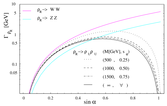
Figure 1: The most important partial widths for the $\rho_{R}$ Higgs boson decay as a function of $s_{\alpha}$ for $m_{\rho_{R}}=300\,\,\;\hbox{GeV}$ and $m_{\rho_{U}}=120\,\,\;\hbox{GeV}$. The continuous magenta (dark gray) line corresponds to the process $\rho_{R}\rightarrow WW$ and the continuous cyan (light gray) line to $\rho_{R}\rightarrow ZZ$. The black lines corresponds to the decay $\rho_{R}\rightarrow\rho_{U}\rho_{U}$ for $(M,s_{\varphi})=(500\,\;\hbox{GeV},0.25)$ (dotted line), $(M,s_{\varphi})=(1000\,\;\hbox{GeV},0.5)$ (dashed line), $(M,s_{\varphi})=(1500\,\;\hbox{GeV},0.75)$ (dash-dotted line) and $M=\infty$ (continuous line).

Let us now study the production cross sections. The Higgstrahlung cross sections for the $\rho_{U}$ and the $\rho_{R}$ are shown in Fig. 2 for $s_{\alpha}=0.25$ (left panel) and for $s_{\alpha}=0.9$ (right panel), with $M=1000\,\,\;\hbox{GeV}\,$, $s_{\varphi}=0.5\,\,$ at a LC with $\sqrt{s}=500\,\,\;\hbox{GeV}$ (black lines), $\sqrt{s}=800\,\,\;\hbox{GeV}$ (magenta (gray) lines).

In general for $s_{\alpha}\gtrsim 0.7$ the production rate for the $\rho_{R}$ can be greater than the $\rho_{U}$ one even if $m_{\rho_{R}}>m_{\rho_{U}}$; this means that, in this case, the heavier Higgs boson $\rho_{R}$ could be detected at a LC before the lighter $\rho_{U}$, (see Fig. 2).

The Higgstrahlung cross section is sensitive to the new vector resonances: in fact for center of mass energies close to $M$ the $\rho_{U}$ production via this mechanism differs from the SM one by a factor that can be much more different from the naive $c_{\alpha}^{2}$ due to the coupling.

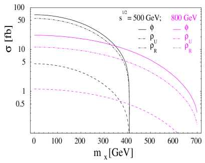
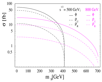
Figure 2: Higgstrahlung cross sections as a function of the Higgs boson mass $m_{X}$ for the L-BESS model $\rho_{U}$ boson (dash-dotted lines) and $\rho_{R}$ boson (dashed lines) , and for the SM $\phi$ boson (continuous lines), with: $\sqrt{s}=500\,\,\;\hbox{GeV}$ (black lines) and $\sqrt{s}=800\,\,\;\hbox{GeV}$ (magenta (gray) lines), $M=1000\,\,\;\hbox{GeV}\,$, $s_{\varphi}=0.5$, $s_{\alpha}=0.25$ (left panel), $s_{\alpha}=0.9$ (right panel).

For increasing values of the energy of the collider the $V^{\pm}V^{\mp}$ fusion process becomes dominant with respect to the Higgstrahlung process. We have computed the fusion cross section by using the code COMPHEP [8]: the results for the production of the Higgs $\rho_{R}$ for $\sqrt{s}=800\,\;\hbox{GeV}$, $s_{\alpha}=0.25$, $(M,s_{\varphi})=(1000\,\;\hbox{GeV},0.25)$, are shown in Table 1 for different values of $m_{\rho_{R}}$. For comparison we also give the Higgstrahlung cross section values. For example, for an integrated luminosity of 1000  fb^-1 and $m_{\rho_{R}}=600\;\hbox{GeV}$, one has 150 fusion events and detection is possible, while for $m_{\rho_{R}}=700\;\hbox{GeV}$ one has only 16 events and an accurate analysis of signal to background ratio is required.

In Table 2 we show the fusion cross section for the process $V^{\pm}V^{\mp}\rightarrow\rho_{U}$ for $\sqrt{s}\ =\ 500\,\;\hbox{GeV}$, $m_{\rho_{U}}=120\,\;\hbox{GeV}$, $s_{\varphi}=0.5$ and different values of $s_{\alpha}$ and $M$. A decrease in the SM Higgs fusion cross section can be the consequence of the presence of new vectors and/or the $c_{\alpha}^{2}$ factor as in the case of the Higgstrahlung process.

$m_{\rho_{R}}[\;\hbox{GeV}]$	100	200	300	400	500	600
$\sigma_{fusionV^{\pm}V^{\mp}}[~{}\mbox{fb}]$	12.0	6.73	3.48	1.60	0.60	0.15
$\sigma_{Higgstrahlung}[~{}\mbox{fb}]$	1.32	1.15	0.90	0.62	0.35	0.15

Table 1: Fusion cross section $V^{\pm}V^{\mp}$ with $V^{\pm}=W^{\pm},V_{L}^{\pm}$ and Higgstrahlung for different values of $m_{\rho_{R}}$ with $\sqrt{s}=800\;\hbox{GeV}$, $s_{\alpha}=0.25$ and $(M,s_{\varphi})=(1000\;\hbox{GeV},0.25)$.

$\sigma_{fusionV^{\pm}V^{\mp}}$	$M=1000\;\hbox{GeV}$	$M=2000\;\hbox{GeV}$	$M=\infty$
$s_{\alpha}=0$	$75.6~{}\mbox{fb}$	$77.4\,\,fb$	$77.9\,\,fb$
$s_{\alpha}=0.25$	$70.7~{}\mbox{fb}$	$72.3\,\,fb$	$73.1\,\,fb$
$s_{\alpha}=0.5$	$56.2~{}\mbox{fb}$	$57.9\,\,fb$	$58.4\,\,fb$

Table 2: Fusion cross section $V^{\pm}V^{\mp}\to\rho_{U}$ with $M=1000\,\,GeV$, $M=2000\;\hbox{GeV}$ and $M=\infty$ for $s_{\alpha}=0$, $s_{\alpha}=0.25$, $s_{\alpha}=0.5$; $\sqrt{s}=500\;\hbox{GeV}$, $s_{\varphi}=0.5$, $m_{\rho_{U}}=120\;\hbox{GeV}$.

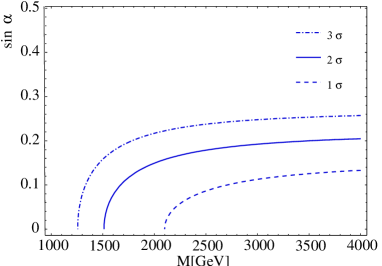
Figure 3: $1\sigma$ (dashed line), $2\sigma$ (continuous line) and $3\sigma$ (dash-dotted line) contours in the plane ($M,s_{\alpha}$) from deviations in the $\rho_{U}$ Higgstrahlung with respect to the SM for $m_{\rho_{U}}=120\;\hbox{GeV}$, $s_{\varphi}=0.5$, $\sqrt{s}=500\;\hbox{GeV}$ and $L=500$ fb^-1.

	$g^{2}_{\rho_{U}WW}$	$g^{2}_{\rho_{U}ZZ}$	$g^{2}_{\rho_{U}bb}$	$g^{2}_{\rho_{U}\tau\tau}$	$g^{2}_{\rho_{U}cc}$	$g^{2}_{\rho_{U}tt}$
$(\Delta g^{2}/g^{2})_{ex}$	2.4%	2.4%	4.4%	6.6%	7.4%	10%
$(\Delta g^{2}/g^{2})_{th}$	-	-	3.5%	-	24%	2.5%
$s_{\alpha}$	0.22	0.22	0.34	0.36	0.71	0.45

Table 3: $s_{\alpha}$ upper bounds assuming a $2\sigma$ deviation (with respect to the SM prediction) in the measurements of squared couplings of a lightest Higgs $\rho_{U}$, with $m_{\rho_{U}}=120\;\hbox{GeV}$, to $WW^{*}$, $ZZ^{*}$, $b\bar{b}$, $\tau^{+}\tau^{-}$, $c\bar{c}$ and $t\bar{t}$ assuming $\sqrt{s}=500\;\hbox{GeV}$, $M>>4000\;\hbox{GeV}$, $s_{\varphi}<<0.5$ and an integrated luminosity of $500~{}\mbox{fb${}^{-1}$}$ except for $tt$ ($\sqrt{s}=800\;\hbox{GeV}$ and $L=1000~{}\mbox{fb${}^{-1}$}$ from $e^{+}e^{-}\to\bar{t}tH$.)

5 Bounds from precision measurements at future LC

A LC besides detecting one or more Higgs bosons can also determine with precision their masses, their couplings to fermions and to gauge bosons and their trilinear couplings. In the scenario where only one light Higgs boson has been discovered these precision measurements allow to get bounds on extended electroweak models like the one we are considering. We have assumed an experimental uncertainty on the determination of the Higgstrahlung cross section $\Delta\sigma/\sigma=2.4\%$ [9]. If no deviation with respect to the prediction of the SM is observed on $\sigma_{Higgstrahlung}$, at a LC with $\sqrt{s}=500\;\hbox{GeV}$ and $L=500$ fb^-1, one gets the bounds in the plane ($M,s_{\alpha}$), shown in Fig. 3. For example, for $M\sim 4\;\hbox{TeV}$, so that the new resonances are not accessible at the LHC, the 95% C.L.limit on $s_{\alpha}$ is $\sim 0.2$.

By combining the fusion cross section, the Higgstrahlung cross section, the measurements of different Higgs branching fractions and $e^{+}e^{-}\to\bar{t}tH$ cross section one can extract the Higgs squared couplings to fermions and gauge bosons or equivalently the partial widths with the experimental uncertainty given in [9, 10]. Assuming no deviations with respect to the SM, the $2\sigma$ upper bounds on $s_{\alpha}$ are given in Table 3. In deriving these limits we have also taken into account the theoretical uncertainties, also given in Table 3. The strongest bounds come from the measurements of $g^{2}_{\rho_{U}WW}$, $g^{2}_{\rho_{U}ZZ}$ and $g^{2}_{\rho_{U}bb}$.

LC measurements of double Higgs production $e^{+}e^{-}\to HHZ$ and $e^{+}e^{-}\to\nu_{e}\bar{\nu}_{e}HH$ can also determine the Higgs trilinear coupling for Higgs masses in the range $120-180~{}GeV$ with an accuracy of 22% (for $\sqrt{s}=500\;\hbox{GeV}$ and $L=1000~{}\mbox{fb${}^{-1}$}$) [9] and of 8% (for a multiTev LC) [11]. Using the expression given in eq. (6) this last bound can be translated in a 2$\sigma$ limit on $s_{\alpha}\sim 0.33$.

6 Conclusions

We have discussed the scalar sector of the linearized version of the BESS model which predicts three scalar states: $\rho_{U}$, $\rho_{R}$ and $\rho_{L}$. The $\rho_{U}$ and $\rho_{R}$ bosons mix and therefore, depending on the mixing angle, can be detected at the LHC and at a LC, instead the $\rho_{L}$ has no coupling to fermions and suppressed couplings to SM gauge bosons. At the LHC the best channel for an heavy Higgs is the $ZZ\to 4\ell$ channel, while at a LC the recoil technique allows the discovery no matter how the $\rho_{R}$ decays. The main decay channels of the $\rho_{R}$ are $WW$ and $\rho_{U}\rho_{U}$ (when kinematically allowed and for small $s_{\alpha}$): therefore detection of $\rho_{R}$ at a LC is possible in a larger region of the parameter space. The LC’s offer, in addition to the detection of the scalar particles, the possibility of discriminating among different models by accurate measurements of the production cross sections and the Higgs couplings, by combining measurements of branching ratios, Higgstrahlung and fusion cross sections.

We wish to thank M. Battaglia for interesting discussions.

References

[1]
M. Schmaltz.
Physics beyond the standard model (theory): Introducing the little Higgs.
Nucl. Phys. Proc. Suppl., 117:40–49, 2003.
[2]
R. S. Chivukula, E. H. Simmons, and J. Terning.
Limits on noncommuting extended technicolor.
Phys. Rev., D53:5258–5267, 1996;
R. S. Chivukula, E. H. Simmons, J. Howard, and H.-J. He.
Precision electroweak constraints on hidden local symmetries.
hep-ph/0304060.
[3]
R. Casalbuoni et al.
Symmetries for vector and axial vector mesons.
Phys. Lett., B349:533–540, 1995;
R. Casalbuoni et al.
Low energy strong electroweak sector with decoupling.
Phys. Rev., D53:5201–5221, 1996.
[4]
R. Casalbuoni, S. De Curtis, D. Dominici, and M. Grazzini.
An extension of the electroweak model with decoupling at low
energy.
Phys. Lett., B388:112–120, 1996;
R. Casalbuoni, S. De Curtis, D. Dominici, and M. Grazzini.
New vector bosons in the electroweak sector: A renormalizable model
with decoupling.
Phys. Rev., D56:5731–5747, 1997.
[5]
R. Casalbuoni, S. De Curtis, and M. Redi.
Signals of the degenerate BESS model at the LHC.
Eur. Phys. J., C18:65–71, 2000.
[6]
R. Casalbuoni and L. Marconi.
The linear BESS model and the double Higgs-strahlung production.
J. Phys., G29:1053–1060, 2003.
[7]
G. F. Gunion, E. H. Howard, G. Kane and S. Dawson.
The Higgs Hunter’s Guide.
Perseus Publishing, 2000.
[8]
A. Pukhov et al.
COMPHEP: A package for evaluation of Feynman diagrams and
integration over multi-particle phase space. User’s manual for version 33.
1999.
[9]
M. Battaglia and K. Desch.
Precision studies of the Higgs boson profile at the Linear
Collider.
hep-ph/0101165.
Batavia 2000, Physics and experiments with future linear
colliders 163-182, 2000.
[10]
J. Conway, K. Desch, J. F. Gunion, S. Mrenna, and D. Zeppenfeld.
The precision of Higgs boson measurements and their implications.
eConf, C010630:P1WG2, 2001.
[11]
M. Battaglia, E. Boos, and W.-M. Yao.
Studying the Higgs potential at the Linear Collider.
eConf, C010630:E3016, 2001.