Status of the CPT Violating Interpretations of the LSND Signal

Abstract

We study the status of the CPT violating neutrino mass spectrum which has been proposed to simultaneously accommodate the oscillation data from LSND, KamLAND, atmospheric and solar neutrino experiments, as well as the non-observation of anti-neutrino disappearance in short-baseline reactor experiments. We perform a three-generation analysis of the global data with the aim of elucidating the viability of this solution. We find no compatibility between the results of the oscillation analysis of LSND and all-but-LSND data sets below 3$\sigma$ CL. Furthermore, the global data without LSND show no evidence for CPT violation: the best fit point of the all-but-LSND analysis occurs very close to a CPT conserving scenario.

I Introduction

The joint explanation of the oscillation signals observed in LSND lsnd , in solar chlorine ; sage ; gallex ; gno ; sksollast ; snoccnc and atmospheric skatmlast ; skatmpub ; macro ; soudan neutrino experiments, and in the KamLAND reactor experiment kamland provides a big challenge to neutrino phenomenology. In Refs. cpt1 ; cpt2 it was observed that the LSND signal could be accommodated with the solar and atmospheric neutrino anomalies without enlarging the neutrino sector if CPT was violated. Once such a drastic modification of standard physics is accepted, oscillations with four independent $\Delta m^{2}$ are possible, two in the neutrino and two in the anti-neutrino sector. The basic realization behind these proposals is that the oscillation interpretation of the solar results involves oscillations of electron neutrinos with $\Delta m^{2}_{\odot}\lesssim 10^{-4}\leavevmode\nobreak\ \text{eV}^{2}$ solarprekam , while the LSND signal for short-baseline oscillations with $\Delta m^{2}_{\text{LSND}}\gtrsim 10^{-1}\leavevmode\nobreak\ \text{eV}^{2}$ stems dominantly from anti-neutrinos ($\overline{\nu}_{\mu}\rightarrow\overline{\nu}_{e}$). If CPT was violated and neutrino and anti-neutrino mass spectra and mixing angles were different cpt1 ; cpt2 ; cpt4 ; cpt5 ; cpt3 both results could be made compatible in addition to the interpretation of the atmospheric neutrino data in terms of oscillations of both $\nu_{\mu}$ and $\overline{\nu}_{\mu}$ with $\Delta m^{2}_{\text{atm}}\sim 10^{-3}\leavevmode\nobreak\ \text{eV}^{2}$ skatmlast .

In the original spectrum proposed, neutrinos had mass splittings $\Delta m^{2}_{\odot}=\Delta m^{2}_{21}\ll\Delta m^{2}_{31}=\Delta m^{2}_{\text{atm}}$ to explain the solar and atmospheric observations, while for anti-neutrinos $\Delta m^{2}_{\text{atm}}=\Delta\overline{m}^{2}_{21}\ll\Delta\overline{m}^{2}_{31}=\Delta m^{2}_{\text{LSND}}$. Within this spectrum the mixing angles could be adjusted to obey the relevant constraints from laboratory experiments, mainly due to the non-observation of reactor $\overline{\nu}_{e}$ at short distances chooz ; bugey , and a reasonable description of the data could be achieved cpt3 ; solveig ; strumia . In general, stronger constraints on the possibility of CPT violation arise, once a specific source of CPT violation which involves other sectors of the theory is invoked cptirina . For a summary of recent theoretical work and experimental tests see, for example, Ref. kostelecky and references therein.

On pure phenomenological grounds, the first test of this scenario came from the KamLAND kamland experiment since the suggested CPT-violating neutrino spectrum allowed to reconcile the solar, atmospheric and LSND anomalies, but, once the constraints from reactor experiments were imposed, no effect in KamLAND was predicted. The observation of a deficit in KamLAND at $3.5\sigma$ CL clearly disfavoured these scenarios. Furthermore, KamLAND results demonstrate that $\overline{\nu}_{e}$ oscillate with parameters consistent with the LMA $\nu_{e}$ oscillation solution of the solar anomaly. This fact by itself can be used to set constraints on the possibility of CPT violation cptjb ; strumia ; cptmura . Within the present KamLAND accuracy, however, the bounds are not very strong because KamLAND data does not show a significant evidence of energy distortion.

The present situation is that the results of solar experiments in $\nu$ oscillations, together with the results from KamLAND and the bounds from other $\bar{\nu}$ reactor experiments show that both neutrinos and anti-neutrinos oscillate with $\Delta m^{2}_{\odot},\Delta m^{2}_{\text{reac}}\leq 10^{-3}\leavevmode\nobreak\ \text{eV}^{2}$. Adding this to the evidence of oscillations of both atmospheric neutrinos and anti-neutrinos with $\Delta m^{2}_{\text{atm}}\sim 10^{-3}\leavevmode\nobreak\ \text{eV}^{2}$, leaves no room for oscillations with $\Delta m^{2}_{\text{LSND}}\sim 1\leavevmode\nobreak\ \text{eV}^{2}$. The obvious conclusion then is that CPT violation can no-longer explain LSND and perfectly fit all other data strumia .

This conclusion relies strongly on the fact that atmospheric oscillations have been observed for both neutrinos and anti-neutrinos with the same $\Delta m^{2}_{\text{atm}}$. However, atmospheric neutrino experiments do not distinguish neutrinos from anti-neutrinos, and neutrinos contribute more than anti-neutrinos to the event rates by a factor $\sim$ 4–2 (the factor decreases for higher energies). Based on this fact, in Ref. cpt5 an alternative CPT-violating spectrum was proposed as shown in Fig. 1. In this scheme only atmospheric neutrinos oscillate with $\Delta m^{2}_{\text{atm}}$ and give most of the contribution to the observed zenith angular dependence of the deficit of $\mu$-like events. Atmospheric $\overline{\nu}_{\mu}$ dominantly oscillate with $\Delta m^{2}_{\text{LSND}}$ which leads to an almost constant (energy and angular independent) suppression of the corresponding events. For low $\overline{\nu}_{\mu}$ energies oscillations with $\Delta m^{2}_{\text{reac}}$ can also be a source of zenith-angular dependence. The claim in Ref. cpt5 was that altogether this suffices to give a good description of the atmospheric data such that the scheme in Fig. 1 can still be a viable solution to all the neutrino puzzles. This conclusion was contradicted in Ref. strumia by an analysis of atmospheric and K2K data. However, according to the authors in Ref. cpt5 an important point to their conclusion was the consideration of the full 3$\nu$ and 3$\overline{\nu}$ oscillations, while the analysis in Ref. strumia was made on the basis of a 2$\nu$+2$\overline{\nu}$ approximation.

In this article we determine the status of the CPT violating scenario in Fig. 1 as an explanation to the existing neutrino anomalies. In order to do this, we perform a three-generation global analysis of the solar, atmospheric, reactor, and long-baseline (LBL) data, and compare the allowed parameter regions from this analysis to the ones required to explain the LSND data. We find that no consistency between the parameters determined by the analyses of both data sets appears below 3$\sigma$ CL.

Figure 1: Post KamLAND CPT violating neutrino mass spectrum proposed in Ref. cpt5 .

II Notation and Data Inputs

In what follows we label the states as in Fig. 1 with $\Delta m^{2}_{ij}=m^{2}_{i}-m^{2}_{j}$ and $\Delta\overline{m}^{2}_{ij}=\overline{m}^{2}_{i}-\overline{m}^{2}_{j}$. We denote by $U$ and $\overline{U}$ the corresponding neutrino and anti-neutrino mixing matrix MNS which we chose to parametrize as PDG

$$U=\left(\begin{array}[]{ccc}c_{13}c_{12}&s_{12}c_{13}&s_{13}\\ -s_{12}c_{23}-s_{23}s_{13}c_{12}&c_{23}c_{12}-s_{23}s_{13}s_{12}&s_{23}c_{13}\\ s_{23}s_{12}-s_{13}c_{23}c_{12}&-s_{23}c_{12}-s_{13}s_{12}c_{23}&c_{23}c_{13}\end{array}\right)\,,$$ (1)

where $c_{ij}\equiv\cos\theta_{ij}$ and $s_{ij}\equiv\sin\theta_{ij}$ and with an “over-bar” for the corresponding anti-neutrino mixing. In writing Eq. (1) we take into account that for our following description it is correct and sufficient to set all the CP phases to zero.

In the anti-neutrino sector the reactor experiments chooz ; bugey ; kamland provide information on the $\overline{\nu}_{e}$ survival probability:

$$\begin{split}P_{ee}^{\text{reac}}&=1-\overline{c}_{13}^{4}\sin^{2}2\overline{\theta}_{12}\sin^{2}\left(\frac{\Delta\overline{m}^{2}_{21}L}{4E}\right)\\ &\hskip 14.22636pt-\sin^{2}2{\overline{\theta}_{13}}\left[\overline{c}_{12}^{2}\sin^{2}\left(\frac{\Delta\overline{m}^{2}_{31}L}{4E}\right)+\overline{s}_{12}^{2}\sin^{2}\left(\frac{\Delta\overline{m}^{2}_{32}L}{4E}\right)\right]\\[8.53581pt] &\simeq\begin{cases}1-\sin^{2}2\overline{\theta}_{13}\sin^{2}\left(\dfrac{\Delta\overline{m}^{2}_{31}L}{4E}\right)&\text{for}\quad\Delta\overline{m}^{2}_{21}L/E\ll 1\\[11.38109pt] \overline{s}_{13}^{4}+\overline{c}_{13}^{4}\left[1-\sin^{2}2\overline{\theta}_{12}\sin^{2}\left(\dfrac{\Delta\overline{m}^{2}_{21}L}{4E}\right)\right]&\text{for}\quad\Delta\overline{m}^{2}_{31}L/E\gg 1\end{cases}\end{split}$$ (2)

In our analysis we include the results from the KamLAND kamland , Bugey bugey and CHOOZ chooz reactor experiments. For KamLAND we include information on the observed anti-neutrino spectrum which accounts for a total of 13 data points. Details of our calculations and statistical treatment of KamLAND data can be found in Ref. ourkland . For reactor experiments performed at short-baselines we include the constraints from Bugey bugey and CHOOZ chooz which are the most relevant for $\Delta\overline{m}^{2}\gtrsim 0.03\leavevmode\nobreak\ \text{eV}^{2}$ and $0.03\leavevmode\nobreak\ \text{eV}^{2}\gtrsim\Delta\overline{m}^{2}\gtrsim 10^{-3}\leavevmode\nobreak\ \text{eV}^{2}$, respectively. In our analysis of the CHOOZ data we include their energy binned data which corresponds to 14 data points (7-bin positron spectra from both reactors, Table 4 in Ref. chooz ) with one constrained normalization parameter. For the analysis of Bugey data we use a total of 60 data points given in Fig. 17 of Ref. bugey , where the ratio of the observed number of events to the one expected for no oscillations is shown for the three distances 15 m, 40 m, and 90 m. For technical details of our Bugey analysis see Ref. tomas31 .

In the scheme under consideration the probability associated with the $\overline{\nu}_{\mu}\to\overline{\nu}_{e}$ signal in LSND is given by

$$P_{\text{LSND}}\equiv\sin^{2}2\theta_{\text{LSND}}\sin^{2}\left(\frac{\Delta m^{2}_{\text{LSND}}L}{4E}\right)=\overline{s}_{23}^{2}\sin^{2}2\overline{\theta}_{13}\,\sin^{2}\left(\frac{\Delta\overline{m}^{2}_{31}L}{4E}\right)\,,$$ (3)

where we have neglected terms proportional to $\Delta\overline{m}^{2}_{21}$ which are irrelevant for LSND distances and energies. In Eq. (3) we have introduced the notation

$$\Delta m^{2}_{\text{LSND}}=\Delta\overline{m}^{2}_{31}\,,\quad\sin^{2}2\theta_{\text{LSND}}=\overline{s}_{23}^{2}\sin^{2}2\overline{\theta}_{13}\,,$$ (4)

which we will use in the presentation of our results. To include LSND we use the results of Ref. church , based only on the decay-at-rest anti-neutrino data sample, which has a high sensitivity to the oscillation signal. The $\chi^{2}_{\text{LSND}}$ is derived from a likelihood function obtained from an event-by-event analysis of the data church . LSND has also studied the neutrino channel $\nu_{\mu}\rightarrow\nu_{e}$ from decay-in-flight events. The full 1993-1998 data sample leads to an oscillation probability for neutrinos of $(0.10\pm 0.16\pm 0.04)\%$ lsnd , which, although consistent with the anti-neutrino signal, is also perfectly consistent with the absence of neutrino oscillations at LSND, as required in the CPT violating scenario. This fact is the first motivation and successful crucial test for the explanation of the LSND results by CPT violation. In view of the low statistical significance of the LSND neutrino signal we do not include it in the analysis.

For the neutrino sector we use information from solar neutrino experiments and the K2K k2kprl LBL experiment. For the solar neutrino analysis we use 80 data points. We include the two measured radiochemical rates, from the chlorine chlorine and the gallium sage ; gallex ; gno experiments, the 44 zenith-spectral energy bins of the electron neutrino scattering signal measured by the SK collaboration sksollast , and the 34 day-night spectral energy bins measured with the SNO snoccnc detector. We take account of the BP00 bp00 predicted fluxes and uncertainties for all solar neutrino sources except for the ⁸B flux which we treat as a free parameter. For the relevant cases oscillations with $\Delta m^{2}_{31}$ are averaged out for solar neutrinos and the survival probability takes the form:

$$P^{3\nu,\rm sol}_{ee}=s^{4}_{13}+c^{4}_{13}\,P^{2\nu,\rm sol}_{ee}(\Delta m^{2}_{21},\theta_{12})\;,$$ (5)

where $P^{2\nu,\rm sol}_{ee}(\Delta m^{2}_{21},\theta_{12})$ is the survival probability for 2$\nu$ mixing obtained with the modified matter density $N_{e}\rightarrow c^{2}_{13}N_{e}$.

The results of the analysis of the solar neutrino data solarprekam imply that $\Delta m^{2}_{21}$ has to be small enough to be irrelevant for the K2K baseline and energy, and the $\nu_{\mu}$ survival probability at K2K is

$$P^{\text{K2K}}_{\mu\mu}=1-4\left(s^{4}_{23}s^{2}_{13}c^{2}_{13}+c^{2}_{13}s^{2}_{23}c^{2}_{23}\right)\sin^{2}\left(\frac{\Delta m^{2}_{32}L}{4E}\right)\,.$$ (6)

In the analysis of K2K we include the data on the normalization and shape of the spectrum of single-ring $\mu$-like events as a function of the reconstructed neutrino energy. The total sample corresponds to 29 events k2kprl . We bin the data in five 0.5 GeV bins with $0<E_{\text{rec}}<2.5$ plus one bin containing all events above $2.5$ GeV. The details of the analysis can be found in Ref. ourthree .

Finally, the analysis of atmospheric neutrino data involves oscillations of both neutrinos and anti-neutrinos, and, in the framework of 3$\nu$+3$\overline{\nu}$ mixing, matter effects become relevant. We solve numerically the evolution equations for neutrinos and anti-neutrinos in order to obtain the corresponding oscillation probabilities for both $e$ and $\mu$ flavours. In our calculations, we use the PREM model of the Earth PREM matter density profile. We include in our analysis all the contained events from the 1489 SK data set skatmlast , as well as the upward-going neutrino-induced muon fluxes from both SK and the MACRO detector macro . This amounts for a total of 65 data points. More technical descriptions of our simulation and statistical analysis can be found in Ref. ouratmos .

III Results

Our basic approach to test the status of the scheme in Fig. 1 as a possible explanation of the LSND anomaly together with all other neutrino and anti-neutrino oscillation data is as follows. First, we perform a global analysis of all the relevant data, but leaving out LSND data. The goal of this analysis is to obtain the allowed ranges of parameters $\Delta m^{2}_{\text{LSND}}$ and $\sin^{2}2\theta_{\text{LSND}}$ as defined in Eq. (4) from this all-but-LSND data set. We then compare these allowed regions to the corresponding allowed parameter region from LSND, and quantify at which CL both regions become compatible.

In this approach we start by defining the most general $\chi^{2}$ for the all-but-LSND data set:

$$\chi^{2}_{\text{all-but-LSND}}(\Delta m^{2}_{21},\Delta m^{2}_{31},\theta_{12},\theta_{23},\theta_{13}|\Delta\overline{m}^{2}_{21},\Delta\overline{m}^{2}_{31},\overline{\theta}_{12},\overline{\theta}_{23},\overline{\theta}_{13})=\chi^{2}_{\text{sol}}(\Delta m^{2}_{21},\theta_{12},\theta_{13})\\ +\chi^{2}_{\text{K2K}}(\Delta m^{2}_{31},\theta_{23},\theta_{13})+\chi^{2}_{\text{Bugey+CHOOZ+KLAND}}(\Delta\overline{m}^{2}_{21},\Delta\overline{m}^{2}_{31},\overline{\theta}_{12},\overline{\theta}_{13})\\ +\chi^{2}_{\text{ATM}}(\Delta m^{2}_{21},\Delta m^{2}_{31},\theta_{12},\theta_{23},\theta_{13}|\Delta\overline{m}^{2}_{21},\Delta\overline{m}^{2}_{31},\overline{\theta}_{12},\overline{\theta}_{23},\overline{\theta}_{13})\,.$$ (7)

Notice that in this comparison we have not included the constraints from the non-observation of $\overline{\nu}_{\mu}\to\overline{\nu}_{e}$ transitions at KARMEN karmen , which, by themselves, disfavour part of the LSND allowed parameter region. The reason for this omission is that we want to test the status of the CPT interpretation of the LSND signal using data independent of the “tension” between LSND and KARMEN results church .

We first focus on the parameters $\Delta m^{2}_{21}$ and $\theta_{12}$. These parameters are dominantly determined by solar neutrino data, which for any $\theta_{13}$ prefer values of $\Delta m^{2}_{21}$ well below the sensitivity of atmospheric neutrino data. Therefore, solar data are mostly important to enforce the “decoupling” of the $\Delta m^{2}_{21}$ oscillations from the problem. In other words, the atmospheric neutrino analysis can be made without any loss of generality, in the standard hierarchical approximation for neutrinos, neglecting the effect $\Delta m^{2}_{21}$ but keeping the generic-3$\nu$ dependence on $\theta_{13}$. Notice that, unlike in the CPT conserving case, in the relevant ranges of mass differences, $\theta_{13}$ is not bounded by any “terrestrial” experiment. The dominant source of information on $\theta_{13}$ is atmospheric data (and less important also solar data), and for this reason we consistently take into account this parameter in our analysis. Thus, after the marginalization over $\Delta m^{2}_{21}$ and $\theta_{12}$ Eq. (7) takes the form

$$\chi^{2}_{\text{all-but-LSND}}(\Delta m^{2}_{31},\theta_{23},\theta_{13}|\Delta\overline{m}^{2}_{21},\Delta\overline{m}^{2}_{31},\overline{\theta}_{12},\overline{\theta}_{23},\overline{\theta}_{13})=\chi^{2}_{\text{sol,marg12}}(\theta_{13})\\ +\chi^{2}_{\text{K2K}}(\Delta m^{2}_{31},\theta_{23},\theta_{13})+\chi^{2}_{\text{Bugey+CHOOZ+KLAND}}(\Delta\overline{m}^{2}_{21},\Delta\overline{m}^{2}_{31},\overline{\theta}_{12},\overline{\theta}_{13})\\ +\chi^{2}_{\text{ATM}}(\Delta m^{2}_{31},\theta_{23},\theta_{13}|\Delta\overline{m}^{2}_{21},\Delta\overline{m}^{2}_{31},\overline{\theta}_{12},\overline{\theta}_{23},\overline{\theta}_{13}).$$ (8)

Let us now discuss the information on $\Delta\overline{m}^{2}_{21}$ from reactor experiments. The observation of the $\overline{\nu}_{e}$ deficit in KamLAND favours $\Delta\overline{m}^{2}_{21}$ values near the best fit $\Delta\overline{m}^{2}_{21}=7\times 10^{-5}\leavevmode\nobreak\ \text{eV}^{2}$. For such small values oscillations with $\Delta\overline{m}^{2}_{21}$ have no effect for atmospheric neutrinos. Therefore, we will start by studying the case $\Delta\overline{m}^{2}_{21}\leq 10^{-4}\leavevmode\nobreak\ \text{eV}^{2}$ in Secs. III.1 and III.2. We will relax this assumption in Sec. III.3, where we investigate also a possible effect of larger values of $\Delta\overline{m}^{2}_{21}$. Notice also, that the case of small $\Delta\overline{m}^{2}_{21}$ is continuously connected to the CPT conserving scenario since it allows for CPT conservation in the “$12$” sector. For ${\Delta\overline{m}^{2}_{21}}\leq 10^{-4}\leavevmode\nobreak\ \text{eV}^{2}$, one can easily marginalize over $\Delta\overline{m}^{2}_{21}$ and $\overline{\theta}_{12}$ and Eq. (8) further simplifies to

$$\chi^{2}_{\text{all-but-LSND}}(\Delta m^{2}_{31},\theta_{23},\theta_{13}|\Delta\overline{m}^{2}_{31},\overline{\theta}_{23},\overline{\theta}_{13})=\chi^{2}_{\text{sol,marg12}}(\theta_{13})+\chi^{2}_{\text{K2K}}(\Delta m^{2}_{31},\theta_{23},\theta_{13})\\ +\chi^{2}_{\text{Bugey+CHOOZ+KLAND,marg$\overline{12}$}}(\Delta\overline{m}^{2}_{31},\overline{\theta}_{13})+\chi^{2}_{\text{ATM}}(\Delta m^{2}_{31},\theta_{23},\theta_{13}|\Delta\overline{m}^{2}_{31},\overline{\theta}_{23},\overline{\theta}_{13}).$$ (9)

Finally, we notice that for any value $\Delta\overline{m}^{2}_{31}\gtrsim 10^{-3}\leavevmode\nobreak\ \text{eV}^{2}$ the results from CHOOZ or, for larger values of $\Delta\overline{m}^{2}_{31}$, from Bugey, imply a strong limit on $\sin^{2}2\overline{\theta}_{13}$, and in order to obtain the $\overline{\nu}_{e}$ disappearance observed in KamLAND $\overline{\theta}_{13}$ has to be small. Within this bound the results of the atmospheric neutrino analysis are almost independent of the exact value of $\overline{\theta}_{13}$ and this parameter can be effectively set to zero in $\chi^{2}_{\text{ATM}}$ without any loss of generality.

For the sake of concreteness we present the quantitative results corresponding to the normal ordering shown in Fig. 1 for both neutrinos and anti-neutrinos. We have verified that the conclusions hold also for the corresponding inverted orderings either for neutrinos and anti-neutrinos. Note that solar and atmospheric data require $|\Delta m^{2}_{21}|\ll|\Delta m^{2}_{31}|$, and reactor and atmospheric data (and furthermore LSND) require $|\Delta\overline{m}^{2}_{21}|\ll|\Delta\overline{m}^{2}_{31}|$. For such hierarchies, the difference between normal and inverted schemes arises mainly from Earth matter effects in the propagation of atmospheric neutrinos and anti-neutrinos, and for the large values of $|\Delta\overline{m}^{2}_{31}|$ required to explain the LSND signal Earth matter effects are irrelevant in the anti-neutrino channel. Within the present experimental accuracy, these effects are not important enough to lead to significant differences in the results of the atmospheric neutrino analysis for direct and inverted orderings (see for instance Ref. nohier ).

III.1 Analysis of all-but-LSND data

Using all the data described above except from the LSND experiment we find the following all-but-LSND best fit point:

$$\Delta m^{2}_{31} =2.8\times 10^{-3}\leavevmode\nobreak\ \text{eV}^{2} \Delta\overline{m}^{2}_{31} =2\times 10^{-3}\leavevmode\nobreak\ \text{eV}^{2}$$

$$\Delta m^{2}_{21} =5.8\times 10^{-5}\leavevmode\nobreak\ \text{eV}^{2} \Delta\overline{m}^{2}_{21} =7.1\times 10^{-5}\leavevmode\nobreak\ \text{eV}^{2}$$

$$s^{2}_{23} =0.5 \overline{s}^{2}_{23} =0.5$$ (10)

$$s^{2}_{13} =0 \overline{s}^{2}_{13} =0.01$$

$$s^{2}_{12} =0.31 \overline{s}^{2}_{12} =0.34$$

with $\chi^{2}_{\text{all-but-LSND,min}}=186.5$ for $238-11=227$ dof. This can be directly compared to the corresponding analysis in the CPT conserving scenario:

$$\Delta m^{2}_{31}=\Delta\overline{m}^{2}_{31} =2.6\times 10^{-3}\leavevmode\nobreak\ \text{eV}^{2}$$

$$\Delta m^{2}_{21}=\Delta\overline{m}^{2}_{21} =7.1\times 10^{-5}\leavevmode\nobreak\ \text{eV}^{2}$$

$$s^{2}_{23}=\overline{s}^{2}_{23} =0.5$$ (11)

$$s^{2}_{13}=\overline{s}^{2}_{13} =0.009$$

$$s^{2}_{12}=\overline{s}^{2}_{12} =0.31$$

with $\chi^{2}_{\text{all-but-LSND,min}}=187$ for $238-6=232$ dof. We conclude that, allowing for different mass and mixing parameters for neutrinos and anti-neutrinos, all-but-LSND data choose a best fit point very close to CPT conservation and maximal $23$ mixing.

Next we illustrate the amount of CPT violation which is still viable. In order to do so we plot in Fig. 2 the allowed regions for the largest neutrino and anti-neutrino mass splittings $\Delta m^{2}_{31}$ versus $\Delta\overline{m}^{2}_{31}$ and the mixing angles $\theta_{23}$ versus $\overline{\theta}_{23}$ and $\theta_{13}$ versus $\overline{\theta}_{13}$ and (after marginalization with respect to all the undisplayed parameters). The different contours correspond to regions allowed at 90%, 95%, 99% and 3$\sigma$ CL for 2 dof ($\Delta\chi^{2}=4.61$, $5.99$, $9.21$, $11.83$, respectively). In general the regions are larger for anti-neutrino parameters as a consequence of their smaller contribution to the atmospheric event rates. In particular $\Delta\overline{m}^{2}_{31}$ can take values below the region of sensitivity of CHOOZ. As a consequence the limit on $\overline{\theta}_{13}$ at high confidence level is very week. Our results for the allowed regions for the largest neutrino and anti-neutrino mass splittings show good qualitative agreement with the 2$\nu$ analyses of Refs. strumia ; skatmlast . In particular we find that within the 2$\nu$ oscillation approximation the atmospheric neutrino analysis rejects the CPT violating scenario at a level close to 4$\sigma$ ($\chi^{2}(\Delta\overline{m}^{2}_{\text{atm}}=\Delta m^{2}_{\text{LSND}})-\chi^{2}(\Delta\overline{m}^{2}_{\text{atm}}=\Delta m^{2}_{\text{atm}})=14$) which is in reasonable agreement with the $\sim$ 5$\sigma$ rejection obtained in Ref. strumia . As expected, the introduction of the 3$\nu$ mixing and the reactor data leads to some quantitative differences in the size of the allowed regions.

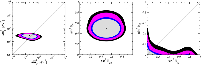
Figure 2: Allowed regions for the largest neutrino and anti-neutrino mass splittings $\Delta m^{2}_{31}$ and $\Delta\overline{m}^{2}_{31}$ and the mixing angles $\theta_{23}$ and $\overline{\theta}_{23}$, and $\theta_{13}$ and $\overline{\theta}_{13}$ (after marginalization with respect to the undisplayed parameters) for $\Delta m^{2}_{21},\Delta\overline{m}^{2}_{21}\leq 10^{-4}\leavevmode\nobreak\ \text{eV}^{2}$ (see text for details). The different contours correspond to the two-dimensional allowed regions at 90%, 95%, 99% and 3$\sigma$ CL from all-but-LSND data. The best fit point is marked with a star.

From our results shown in Eqs. (10), (11) and in Fig. 2 we conclude that current global neutrino oscillation data excluding LSND show no evidence for CPT violation, since the best fit point is very close to a CPT conserving scenario. However, from present data a sizable amount of CPT violation by neutrino parameters is allowed (for a recent discussion on the comparison with the limits existing on the $K-\overline{K}$ mass difference PDG see Ref. cptmura ). We note that it will be possible to significantly improve the limits on CPT violation in the neutrino sector by future experiments such as neutrino factories, see for example Ref. cptnufact .

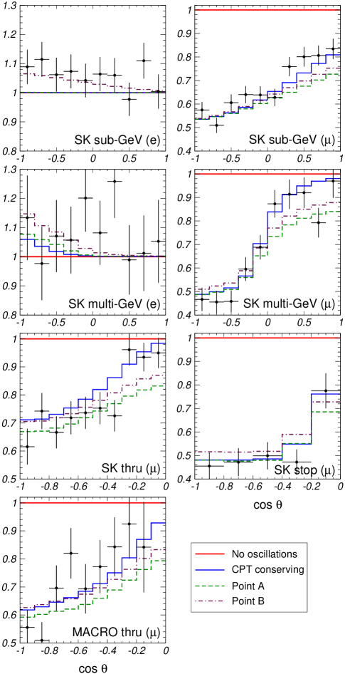
Figure 3: Zenith-angle distributions (normalized to the no-oscillation prediction) for the Super–Kamiokande $e$-like and $\mu$-like contained events, for the Super–Kamiokande stopping and through-going muon events and for Macro up-going muons. The full line gives the distribution for the best fit of $\nu_{\mu}\rightarrow\nu_{\tau}$ oscillations and CPT conservation: $\Delta m^{2}_{31}=\Delta\overline{m}^{2}_{31}=2.6\times 10^{-3}\leavevmode\nobreak\ \text{eV}^{2}$, $s^{2}_{23}=\overline{s}_{23}^{2}=0.5$, $s^{2}_{13}=\overline{s}_{13}^{2}=0$, and $\Delta m^{2}_{21}=\Delta\overline{m}^{2}_{21}\lesssim 10^{-4}\leavevmode\nobreak\ \text{eV}^{2}$. The lines label as “Point A” and “Point B” are the expected distributions for typical LSND–compatible CPT violating cases with the following parameter values: Point A: $\Delta m^{2}_{31}=2.5\times 10^{-3}\leavevmode\nobreak\ \text{eV}^{2}$, $\Delta\overline{m}^{2}_{31}=0.9\leavevmode\nobreak\ \text{eV}^{2}$, $s^{2}_{23}=\overline{s}_{23}^{2}=0.5$, $s^{2}_{13}=0.05$, $\overline{s}_{13}^{2}=0.005$, $\Delta m^{2}_{21}\lesssim 10^{-4}\leavevmode\nobreak\ \text{eV}^{2}$, and $\Delta\overline{m}^{2}_{21}\lesssim 10^{-4}\leavevmode\nobreak\ \text{eV}^{2}$; Point B: $\Delta m^{2}_{31}=2.5\times 10^{-3}\leavevmode\nobreak\ \text{eV}^{2}$, $\Delta\overline{m}^{2}_{31}={\cal O}(\text{eV}^{2})$, $s^{2}_{23}=0.5$, $\overline{s}_{23}^{2}=0.25$, $s^{2}_{13}=0.05$, $\overline{s}_{13}^{2}=0.005$, $\Delta m^{2}_{21}\lesssim 10^{-4}\leavevmode\nobreak\ \text{eV}^{2}$, $\Delta\overline{m}^{2}_{21}=5\times 10^{-4}\leavevmode\nobreak\ \text{eV}^{2}$, and $\overline{s}_{12}^{2}=0.75$.

Concerning LSND, we find that values of $\Delta\overline{m}^{2}_{31}=\Delta\overline{m}^{2}_{\text{LSND}}$ large enough to fit the LSND result do not appear as part of the 3$\sigma$ CL allowed region of the all-but-LSND analysis which is bounded to $\Delta\overline{m}^{2}_{31}<1.6\times 10^{-2}\leavevmode\nobreak\ \text{eV}^{2}$. The upper bound on $\Delta\overline{m}^{2}_{31}$ is determined by atmospheric neutrino data (and slightly strengthened by the reactor constraints). To illustrate the physics behind this result we show in Fig. 3 the zenith-angle distributions of various atmospheric data samples for “Point A” with the following parameter values: $\Delta m^{2}_{31}=2.5\times 10^{-3}\leavevmode\nobreak\ \text{eV}^{2}$, $\Delta\overline{m}^{2}_{31}=0.9\leavevmode\nobreak\ \text{eV}^{2}$, $s^{2}_{23}=\overline{s}_{23}^{2}=0.5$, $s^{2}_{13}=0.05$, $\overline{s}_{13}^{2}=0.005$, $\Delta m^{2}_{21}\lesssim 10^{-4}\leavevmode\nobreak\ \text{eV}^{2}$, and $\Delta\overline{m}^{2}_{21}\lesssim 10^{-4}\leavevmode\nobreak\ \text{eV}^{2}$. This point has been chosen to be compatible with the LSND result while keeping an optimized $\chi^{2}_{\text{all-but-LSND}}$. As seen in the figure this point fails in reproducing the up-down asymmetry of multi-GeV muons as a consequence of the angular-independence in the deficit of the anti-neutrino events. Furthermore, it predicts a too large deficit of up-going muon events near the horizon since $\overline{\nu}_{\mu}$ oscillations with $\Delta\overline{m}^{2}_{31}=0.9\leavevmode\nobreak\ \text{eV}^{2}$ lead to the disappearance of $\overline{\nu}_{\mu}$’s even at those higher energies and shorter distances. For up-going muons the contribution from anti-neutrino events is only half of that from neutrino events. As a consequence this data sample is most sensitive to the anti-neutrino oscillation parameters. Both effects, the wash out of the up-down asymmetry and the deficit of horizontally arriving up-going muons, contribute in comparable amounts to the statistical disfavouring of the CPT violating scenario.

III.2 Comparison of the all-but-LSND and the LSND data sets

It is clear from these results that the CPT violation scenario cannot give a good description of the LSND data and simultaneously fit all-but-LSND results. The quantification of this statement is displayed in Fig. 4 where we show the allowed regions in the ($\Delta\overline{m}^{2}_{31}=\Delta m^{2}_{\text{LSND}}$, $\sin^{2}2\theta_{\text{LSND}}$) plane required to explain the LSND signal together with the corresponding allowed regions from our global analysis of all-but-LSND data.

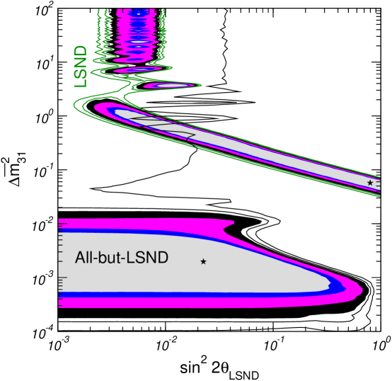
Figure 4: 90%, 95%, 99%, and $3\sigma$ CL allowed regions (filled) in the ($\Delta\overline{m}^{2}_{31}=\Delta m^{2}_{\text{LSND}}$, $\sin^{2}2\theta_{\text{LSND}}$) plane required to explain the LSND signal together with the corresponding allowed regions from our global analysis of all-but-LSND data. The contour lines correspond to $\Delta\chi^{2}=13$ and 16 (3.2$\sigma$ and 3.6$\sigma$, respectively).

Fig. 4 illustrates that below 3$\sigma$ CL there is no overlap between the allowed region of the LSND analysis and the all-but-LSND one, and that for this last one the region is restricted to $\Delta\overline{m}^{2}_{31}=\Delta m^{2}_{\text{LSND}}<0.02\leavevmode\nobreak\ \text{eV}^{2}$. At higher CL values of $\Delta\overline{m}^{2}_{31}\sim{\cal O}(\text{eV}^{2})$ become allowed – as determined mainly by the constraints from Bugey – and an agreement becomes possible. We find that in the neighbourhood of $\Delta\overline{m}^{2}_{31}=\Delta m^{2}_{\text{LSND}}=0.9\leavevmode\nobreak\ \text{eV}^{2}$ and $\sin^{2}2\theta_{\text{LSND}}=0.01$ the LSND and the all-but-LSND allowed regions start having some marginal agreement slightly above 3$\sigma$ CL (at $\Delta\chi^{2}=12.2$). A less fine-tuned agreement appears at 3.3$\sigma$ CL ($\Delta\chi^{2}\sim 14)$ for $\Delta\overline{m}^{2}_{31}=\Delta m^{2}_{\text{LSND}}\gtrsim 0.5\leavevmode\nobreak\ \text{eV}^{2}$ and $\sin^{2}2\theta_{\text{LSND}}\lesssim 0.01$ .

Alternatively the quality of the joint description of LSND and all the other data can be evaluated by performing a global fit based on the total $\chi^{2}$-function $\chi^{2}_{\text{tot}}=\chi^{2}_{\text{all-but-LSND}}+\chi^{2}_{\text{LSND}}$, and applying a goodness-of-fit test. The best fit point of the global analysis is $\sin^{2}2\theta_{\text{LSND}}=6.3\times 10^{-3}$ and $\Delta\overline{m}^{2}_{31}=0.89\leavevmode\nobreak\ \text{eV}^{2}$ with $\chi^{2}_{\text{tot,min}}=200.9$. In the following we will use the so-called parameter goodness-of-fit fourlast ; PG , which is particularly suitable to test the compatibility of independent data sets. Applying this method to the present case we consider the statistic

$$\begin{split}\bar{\chi}^{2}&\equiv\chi^{2}_{\text{tot,min}}-\chi^{2}_{\text{all-but-LSND,min}}-\chi^{2}_{\text{LSND,min}}\\ &=\Delta\chi^{2}_{\text{all-but-LSND}}(\mathrm{b.f.})+\Delta\chi^{2}_{\text{LSND}}(\mathrm{b.f.})\,,\end{split}$$ (12)

where b.f. denotes the global best fit point. The $\bar{\chi}^{2}$ of Eq. (12) has to be evaluated for 2 dof, corresponding to the two parameters $\sin^{2}2\theta_{\text{LSND}}$ and $\Delta\overline{m}^{2}_{31}=\Delta m^{2}_{\text{LSND}}$ coupling the two data sets: all-but-LSND and LSND (see Ref. PG for details about the parameter goodness-of-fit). From $\Delta\chi^{2}_{\text{all-but-LSND}}=12.7$ and $\Delta\chi^{2}_{\text{LSND}}=1.7$ we obtain $\bar{\chi}^{2}=14.4$ leading to the marginal parameter goodness-of-fit of $7.5\times 10^{-4}$.

III.3 The effect of large $\Delta\overline{m}^{2}_{21}$

Finally, we study whether the conclusions of the previous subsections could be affected by allowing for larger values of $\Delta\overline{m}^{2}_{21}$, such that its effect can show up in the atmospheric neutrino data and improve the quality of the fit as suggested in Ref. cpt5 . In Fig. 5 we show the dependence on $\Delta\overline{m}^{2}_{21}$ of the $\chi^{2}$ obtained for the analysis of atmospheric and CHOOZ data, and for all-but-LSND data. In each curve we have marginalized with respect to the undisplayed variables subject to the condition $\Delta\overline{m}^{2}_{31}\gtrsim 1\leavevmode\nobreak\ \text{eV}^{2}$. For the sake of normalization we have subtracted in each case the corresponding $\chi^{2}_{\text{min,CPT}}$ for the CPT conserving scenario.

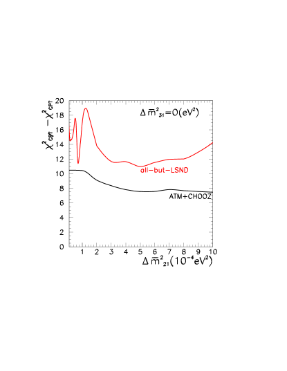
Figure 5: $\Delta\chi^{2}=\chi^{2}_{\text{min,C/\!\!PT}}-\chi^{2}_{\text{min, CPT}}$ as a function of $\Delta\overline{m}^{2}_{21}$ from the analysis of atmospheric+CHOOZ data (lower line) and from all-but-LSND (upper line) data (see text for details).

The figure shows that, indeed, considering only atmospheric+CHOOZ data there is an improvement (although mild) in the quality of the fit due to the effect of oscillations with larger values of $\Delta\overline{m}^{2}_{21}$. To illustrate this result we show in Fig. 3 the zenith-angle distributions of various atmospheric data samples for “Point B”, which gives the lowest $\chi^{2}_{\text{all-but-LSND}}$ for a larger value of $\Delta\overline{m}^{2}_{21}$: $\Delta m^{2}_{31}=2.5\times 10^{-3}\leavevmode\nobreak\ \text{eV}^{2}$, $\Delta\overline{m}^{2}_{31}={\cal O}(\text{eV}^{2})$, $s^{2}_{23}=0.5$, $\overline{s}_{23}^{2}=0.25$, $s^{2}_{13}=0.05$, $\overline{s}_{13}^{2}=0.005$, $\Delta m^{2}_{21}\lesssim 10^{-4}\leavevmode\nobreak\ \text{eV}^{2}$, $\Delta\overline{m}^{2}_{21}=5\times 10^{-4}\leavevmode\nobreak\ \text{eV}^{2}$, and $\overline{s}_{12}^{2}=0.75$. The figure shows that the main effect of $\Delta\overline{m}^{2}_{21}$ oscillations is to increase the number of contained $e$-like events, in particular sub-GeV nohier ; smirnov , improving the fit for those events. However, the two main sources of discrepancy in the atmospheric fit in these scenarios – the small up-down asymmetry for multi-GeV muon-like events and the deficit of horizontally arriving up-going muons – remain a problem even when atmospheric anti-neutrino oscillations with the two relevant wavelengths are included. We conclude from this analysis that the claim in Ref. cpt5 of a possible improvement of the atmospheric neutrino fit due to the inclusion of the effect of oscillations with larger values of $\Delta\overline{m}^{2}_{21}$ is qualitatively correct for the contained events, although quantitatively relevant only for the sub-GeV $e$-like events. Moreover, we find that quantitatively the improvement in the fit is not enough to make the scenario viable. This conclusion is partially based on the bad description of the upward-going muon events in the CPT violating scenario, a fact which was overlooked in Ref. cpt5 .

In other words, our results show that atmospheric neutrino data are precise enough to be sensitive to the anti-neutrino oscillation parameters, and it cannot be well described by a combination of neutrino oscillations with $\Delta m^{2}_{31}\simeq 3\times 10^{-3}\leavevmode\nobreak\ \text{eV}^{2}$ and anti-neutrino two-wavelength oscillations with $\Delta\overline{m}^{2}_{31}\sim{\cal O}(\text{eV}^{2})$ and $\Delta\overline{m}^{2}_{21}\sim$ few $10^{-4}\leavevmode\nobreak\ \text{eV}^{2}$.

The net effect in the global all-but-LSND analysis is that the improvement in the atmospheric fit is not enough to make the scenarios viable because it does not fully overcome the preference of smaller $\Delta\overline{m}^{2}_{21}$ in KamLAND (even within their present limited statistics) as illustrated in the all-but-LSND curve in Fig. 5. The local minimum at $\Delta\overline{m}^{2}_{21}=7.1\times 10^{-5}\leavevmode\nobreak\ \text{eV}^{2}$ corresponds to a point in the vicinity of the point where the LSND and all-but-LSND regions in Fig. 4 first meet. From the curve in Fig. 5 we see that the improvement obtained by moving to the minimum at $\Delta\overline{m}^{2}_{21}=5\times 10^{-4}\leavevmode\nobreak\ \text{eV}^{2}$ is only 0.5 units in $\chi^{2}$. We conclude that higher $\Delta\overline{m}^{2}_{21}$ values do not significantly affect the overall status of the CPT violating scenario.

IV Conclusions

We have explored the possibility of explaining all the existing neutrino anomalies without enlarging the neutrino sector but allowing for CPT violation as described by the scenario in Fig. 1. In order to do so we have performed a compatibility test between the results of the oscillation analysis of the LSND on one side and all-but-LSND data on the other in the framework of 3$\nu$+3$\overline{\nu}$ oscillations. Our main results are shown in Fig. 4. We find that the allowed regions for both data sets have no overlap at 3$\sigma$ CL. Alternatively, using the so-called parameter goodness-of-fit our results imply that the probability for compatibility between both data sets within this scenario is only $7.5\times 10^{-4}$.

The information most relevant to our conclusion comes from the atmospheric neutrino events. Our results show that, within the constraints imposed by solar and LBL neutrino data, and reactor anti-neutrino experiments, atmospheric data are precise enough to be sensitive to anti-neutrino oscillation parameters and cannot be described with oscillations with the wavelengths required in the CPT violating scenario.

Furthermore, the global oscillation data without LSND show no evidence for any CPT violation. An analysis of the all-but-LSND data set allowing for different mass and mixing parameters of neutrinos and anti-neutrinos gives a best fit point very close to perfect CPT conservation.

- (1) A. Aguilar et al. [LSND Collaboration], Phys. Rev. D 64, 112007 (2001).
- (2) Q. R. Ahmad et al., Phys. Rev. Lett. 87, 071301 (2001); Q. R. Ahmad et al., ibid. 89 011301 (2002).
- (3) S. Fukuda et al. [Super-Kamiokande Collaboration], Phys. Lett. B 539, 179 (2002).
- (4) B. T. Cleveland et al., Astrophys. J. 496, 505 (1998).
- (5) J. N. Abdurashitov et al., J. Exp. Theor. Phys. 95, 181 (2002).
- (6) GALLEX collaboration, W. Hampel et al., Phys. Lett. B 447, 127 (1999).
- (7) GNO collaboration, E. Bellotti, Nuclear Phys. B (Proc. Suppl.) 91, 44 (2001).
- (8) M.Shiozawa, SuperKamiokande Coll., in XXth International Conference on Neutrino Physics and Astrophysics, Munich May 2002, (http://neutrino2002.ph.tum.de).
- (9) Y. Fukuda et al., Phys. Lett. B433, (1998) 9; Phys. Lett. B436, (1998) 33; Phys. Lett. B467, (1999) 185; Phys. Rev. Lett. 82, (1999) 2644.
- (10) M.Ambrosio et al., MACRO Coll., Phys. Lett. B 517, (2001) 59.
- (11) D. A. Petyt [SOUDAN-2 Collaboration], Nucl. Phys. Proc. Suppl. 110, 349 (2002).
- (12) K. Eguchi et al. [KamLAND Collaboration], Phys. Rev. Lett. 90, 021802 (2003).
- (13) H. Murayama and T. Yanagida, Phys. Lett. B 520, 263 (2001).
- (14) G. Barenboim, L. Borissov, J. Lykken and A. Y. Smirnov, JHEP 0210, 001 (2002).
- (15) J. N. Bahcall, M. C. Gonzalez-Garcia and C. Pena-Garay, JHEP 0207, 054 (2002). M. Maltoni, T. Schwetz, M.A. Tortola and J.W.F. Valle, Phys. Rev. D 67, 013011 (2003); V. Barger, D. Marfatia, K. Whisnant and B.P. Wood, Phys. Lett. B 537 (2002) 179; P. Creminelli, G. Signorelli and A. Strumia, JHEP 05 (2001), 052; [hep-ph/0102234, see addendum 04/22/2002]; G.L. Fogli, E. Lisi, A. Marrone, D. Montanino and A. Palazzo, Phys. Rev. D 66 (2002) 053010; A. Bandyopadhyay, S. Choubey, S. Goswami and D.P. Roy, Phys. Lett. B 540 (2002) 14; P.C. de Holanda and A.Yu. Smirnov, Phys. Rev. D 66, 113005 (2002).
- (16) G. Barenboim and J. Lykken, Phys. Lett. B 554, 73 (2003).
- (17) G. Barenboim, L. Borissov and J. Lykken, hep-ph/0212116.
- (18) G. Barenboim, L. Borissov and J. Lykken, Phys. Lett. B 534, 106 (2002).
- (19) M. Apollonio et al., Phys. Lett. B 466, 415 (1999).
- (20) Y. Declais et al., Nucl. Phys. B 434, 503 (1995).
- (21) A. Strumia, Phys. Lett. B 539, 91 (2002), hep-ph/0201134.
- (22) S. Skadhauge, Nucl. Phys. B 639, 281 (2002).
- (23) See for example, I. Mocioiu and M. Pospelov, Phys. Lett. B 534, 114 (2002); A. De Gouvea, Phys. Rev. D 66 (2002) 076005; O.W. Greenberg, Phys. Rev. Lett. 89, 231602 (2002).
- (24) V.A. Kostelecky, ed., CPT and Lorentz Symmetry II, World Scientific, Singapore, 2002.
- (25) J. N. Bahcall, V. Barger and D. Marfatia, Phys. Lett. B 534, 120 (2002).
- (26) H. Murayama, hep-ph/0307127.
- (27) B. Pontecorvo, J. Exptl. Theoret. Phys. 33, 549 (1957) [Sov. Phys. JETP 6, 429 (1958)]; Z. Maki, M. Nakagawa and S. Sakata, Prog. Theo. Phys. 28, (1962) 870 ; M. Kobayashi and T. Maskawa, Prog. Theor. Phys. 49, (1973) 652.
- (28) Particle Data Group, D. E. Groom et al., Eur. Phys. J.C15, (2000) 1.
- (29) J. N. Bahcall, M. C. Gonzalez-Garcia and C. Pena-Garay, JHEP 0302, 009 (2003); M. Maltoni, T. Schwetz and J. W. Valle, Phys. Rev. D 67, 093003 (2003).
- (30) W. Grimus and T. Schwetz, Eur. Phys. J. C 20, 1 (2001).
- (31) E. D. Church, K. Eitel, G. B. Mills and M. Steidl, Phys. Rev. D 66 (2002) 013001.
- (32) C. Athanassopoulos et al. [LSND Collaboration], Phys. Rev. C 58 (1998) 2489.
- (33) M. H. Ahn et al., Phys. Rev. Lett. 90, 041801 (2003).
- (34) J. N. Bahcall, M. H. Pinsonneault, and S. Basu, Astrophys. J. 555, 990 (2001).
- (35) M. C. Gonzalez-Garcia and C. Pena-Garay, hep-ph/0306001.
- (36) A.M. Dziewonski and D.L. Anderson, Phys. Earth Planet. Inter. 25, (1981) 297.
- (37) N. Fornengo, M. C. Gonzalez-Garcia and J. W. Valle, Nucl. Phys. B 580, 58 (2000); M. C. Gonzalez-Garcia, H. Nunokawa, O. L. Peres and J. W. Valle, Nucl. Phys. B 543, 3 (1999); M. C. Gonzalez-Garcia, H. Nunokawa, O. L. Peres, T. Stanev and J. W. Valle, Phys. Rev. D 58, 033004 (1998); M. C. Gonzalez-Garcia, M. Maltoni, C. Pena-Garay and J. W. Valle, Phys. Rev. D 63, 033005 (2001).
- (38) B. Armbruster et al., KARMEN Coll., Phys. Rev. D 65 (2002) 112001.
- (39) M. C. Gonzalez-Garcia and M. Maltoni, Eur. Phys. J. C 26, 417 (2003).
- (40) S. M. Bilenky, M. Freund, M. Lindner, T. Ohlsson and W. Winter, Phys. Rev. D 65 (2002) 073024.
- (41) M. Maltoni, T. Schwetz, M. A. Tortola and J. W. Valle, Nucl. Phys. B 643, 321 (2002).
- (42) M. Maltoni and T. Schwetz, Phys. Rev. D 68, 033020 (2003).
- (43) O. L. Peres and A. Y. Smirnov, Phys. Lett. B 456, 204 (1999); Nucl. Phys. Proc. Suppl. 110, 355 (2002).