The flavor asymmetry of the polarized light sea, $\Delta\bar{u}-\Delta\bar{d}$, discriminates between different model calculations of helicity densities. We show that the chiral chromodielectric model, differently from models based on a $1/N_{c}$ expansion, predicts a small value for this asymmetry, what seems in agreement with preliminary HERMES data.

1. Following the discovery that the quark contribution to the spin of the nucleon is surprisingly small [1], a considerable experimental effort was made to elucidate the details of the helicity densities of valence, sea and glue (for reviews on longitudinal spin physics, see [2]). On the other theoretical side, many models have been studied and most of them reproduce the gross features of the spin content of the nucleon, namely the $g_{1}$ structure function and the singlet distribution $\Delta\Sigma=\sum_{f}(\Delta f+\Delta\bar{f})$. In order to discriminate between the models, one has to look at the quark and antiquark helicity densities for each separate flavor. This has been a lacking piece of information until last year, when the HERMES Collaboration at DESY, measuring semi-inclusive deep inelastic scattering, succeeded in extracting the polarizations of $u,\bar{u},d,\bar{d},s+\bar{s}$ [3]. Thus, HERMES experiment opened for the first time the possibility to test model results against data. To this purpose, non-singlet distributions are especially interesting because their evolution does not involve the polarized gluon density: as a consequence, they can be predicted in a more reliable way, without any extra assumption on the constituent polarized glue.

In what follows, our attention will be directed to the isoscalar and isovector combinations of antiquark densities,

$$\bar{f}_{+}(x)=\bar{u}(x)+\bar{d}(x)\,,\;\;\;\qquad\quad\bar{f}_{-}(x)=\bar{u}(x)-\bar{d}(x)\,,$$ (1)

$$\Delta\bar{f}_{+}(x)=\Delta\bar{u}(x)+\Delta\bar{d}(x)\,,\;\;\;\;\;\Delta\bar{f}_{-}(x)=\Delta\bar{u}(x)-\Delta\bar{d}(x)\,.$$ (2)

The two classes of models most widely used for computing quark distributions, i.e. the chiral quark soliton model (CQSM, based on a $1/N_{c}$ expansion) and the bag-like confinement models – including the chiral chromodielectric model (CDM) –, make very different predictions for the relative weight of $\Delta\bar{f}_{-}$ and $\Delta\bar{f}_{+}$, and of $\bar{f}_{+}$ and $\bar{f}_{-}$. In particular, in the $1/N_{c}$ expansion, $\Delta\bar{f}_{-}$ is a leading quantity compared to $\Delta\bar{f}_{+}$ and $\bar{f}_{-}$, hence it is expected to be large (in absolute value) and to satisfy the inequalities (which may be, as a matter of fact, strong inequalities)

$$|\Delta\bar{u}-\Delta\bar{d}|>|\bar{u}-\bar{d}|\,,$$ (3)

$$|\Delta\bar{u}-\Delta\bar{d}|>|\Delta\bar{u}+\Delta\bar{d}|\,.$$ (4)

On the contrary, we shall show that the chromodielectric model predicts a small value for the polarized flavor asymmetry $\Delta f_{-}$, and reversed signs for the inequalities (3, 4). The HERMES preliminary data, although affected by relatively large uncertainties, seem indeed to favor a small $\Delta f_{-}$.

2. Let us start from the field-theoretical expressions of the quark and antiquark helicity distributions, i.e.

$$\Delta f(x) = \int\frac{{\rm d}\xi^{-}}{4\pi}e^{ixp^{+}\xi^{-}}\langle N|\overline{\psi}(0)\gamma^{+}\gamma_{5}\psi(0,\xi^{-},0_{\perp})|N\rangle\,,$$ (5)

$$\Delta\bar{f}(x) = \int\frac{{\rm d}\xi^{-}}{4\pi}e^{ixp^{+}\xi^{-}}\langle N|{\rm Tr}\,\gamma^{+}\gamma_{5}\psi(0)\overline{\psi}(0,\xi^{-},0_{\perp})|N\rangle\,.$$ (6)

Quark models provide the matrix elements in the nucleon state, which cannot be calculated in perturbative QCD.

In a (projected) mean-field approximation, eqs. (5, 6) can be rewritten in terms of single–particle quark or antiquark matrix elements. For the quark distribution one has [4, 5, 6] (the expression for antiquarks is similar)

$$\Delta f(x) =\frac{1}{\sqrt{2}}\sum_{\alpha}\sum_{m}P(f,\alpha,m)$$ (7)

$$\times \,\int\frac{{\rm d}^{3}\mbox{\boldmath$p$}_{\alpha}}{(2\pi)^{3}\,2p_{\alpha}^{0}}\,A_{\alpha}(p_{\alpha})\,\delta[(1-x)\,p^{+}-p^{+}_{\alpha}]\,\overline{\varphi}(p_{\alpha},m)\gamma^{+}\gamma_{5}\,\varphi(p_{\alpha},m)\,,$$

where $\varphi$ is the single-quark wave function, $m$ is the projection of the quark spin along the direction of the nucleon’s spin, $P(f,\alpha,m)$ is the probability of extracting a quark of flavor $f$ and spin $m$ leaving a state generically labeled by the quantum number $\alpha$. The overlap function $A_{\alpha}(p_{\alpha})$ contains the details of the intermediate states and of the projection used to obtain a nucleon with definite linear momentum from a three–quark bag (see for instance [4, 5]). The intermediate states which contribute to (7) are $2q$ and $3q1\bar{q}$ states for the quark distribution, and $4q$ states for the antiquark distribution.

The model of the nucleon that we adopt is the chiral chromodielectric model (CDM) [7]. The Lagrangian of the CDM is

$${\mathcal{L}} = i\bar{\psi}\gamma^{\mu}\partial_{\mu}\psi+{g\over\chi}\,\bar{\psi}\left(\sigma+i\gamma_{5}\mbox{\boldmath$\tau\cdot\pi$}\right)\psi$$ (8)

$$+ {1\over 2}{\left(\partial_{\mu}\chi\right)}^{2}-{1\over 2}M^{2}\chi^{2}+{1\over 2}{\left(\partial_{\mu}\sigma\right)}^{2}+{1\over 2}{\left(\partial_{\mu}\mbox{\boldmath$\pi$}\right)}^{2}-U\left(\sigma,\mbox{\boldmath$\pi$}\right)\,,$$

where $U(\sigma,\mbox{\boldmath$\pi$})$ is the usual mexican-hat potential. ${\mathcal{L}}$ describes a system of interacting quarks, pions, sigmas and a scalar-isoscalar chiral singlet field $\chi$. The parameters of the model are: the chiral meson masses $m_{\pi}=0.14$ GeV, $m_{\sigma}=1.2$ GeV, the pion decay constant $f_{\pi}=93$ MeV, the quark–meson coupling constant $g$, and the mass $M$ of the $\chi$ field. The parameters $g$ and $M$, which are the only free parameters of the model, are fixed by reproducing the average nucleon-delta mass and the isoscalar radius of the proton. The technique used to compute the physical nucleon state $|N\rangle$ is based on a double projection of the mean-field solution on linear and angular momentum eigenstates. It is a standard procedure and we refer the reader to [8] for details about it.

An important point to notice is that the intermediate states labeled by $\alpha$ in eq. (7) are computed within the CDM in a parameter-free manner. The flavor asymmetries of the distribution functions arise from the differences between the intermediate states left out by a $u$ or a $d$ quark (antiquark) (the relevant formalism can be found in Ref.[4]) and therefore the results for these asymmetries are genuine predictions of the model. The two sources of the flavor asymmetry in this approach are therefore the Pauli principle and the splitting of the masses of the intermediate $4q$ states, due to pion exchange corrections. A crucial check of the reliability of our calculation comes from the fulfillment of the valence number sum rule, that we found to be saturated within few percent [5, 9]. Another non-trivial test is provided by the Soffer inequality [10], which turns out to be satisfied by all quark and antiquark distributions of our model.

Finally, we recall that the distributions computed in a quark model describe the nucleon at some low scale $\mu^{2}$ (the “model scale”). They are used as the input of the Altarelli–Parisi evolution from $\mu^{2}$ to a larger scale. In previous works [5, 6] we determined the model scale by comparing the model prediction for the valence momentum with the experimental value and found $\mu^{2}=0.16$ GeV².

3. We computed various combinations of the isovector and isoscalar distributions (1, 2). Our result for the polarized flavor asymmetry $\Delta\bar{f}_{-}=\Delta\bar{u}-\Delta\bar{d}$, evolved in leading-order QCD to the momentum scale of HERMES data, $Q^{2}=2.5$ GeV², is shown in Fig. 1 (solid line). We find that $\Delta\bar{f}_{-}$ is quite small and essentially zero for $x\mathrel{\hbox to0.0pt{\lower 4.0pt\hbox{\hskip 1.0pt$\sim$}\hss}\raise 1.0pt\hbox{$>$}}0.1$. In Fig. 2 we plot the ratio of the polarized to the unpolarized asymmetry, $(\Delta\bar{u}-\Delta\bar{d})/(\bar{d}-\bar{u})$, at $Q^{2}=2.5$ GeV². This ratio is less than unity in the whole $x$ range (for the meaning of the data points in Fig. 2, see below). Finally, Fig. 3 shows the isovector to isoscalar ratio $\Delta\bar{f}_{-}/\Delta\bar{f}_{+}$ predicted by the CDM at the model scale $\mu^{2}$ and at the scale of the HERMES experiment. This ratio must be taken with a grain of salt, since $\Delta\bar{f}_{+}$ has been evolved under the hypothesis of vanishing gluon polarization at the starting scale, which might be a simplistic assumption.

We must recall that a negative feature of the CDM is that it yields single-quark wave functions that are very much peaked in momentum space. Therefore quark distribution functions vanish too rapidly, typically above $x\sim 0.6$. Also antiquark distributions vanish very fast. However, we expect that the ratios presented in Figs. 2–3 should not be much affected by this behavior.

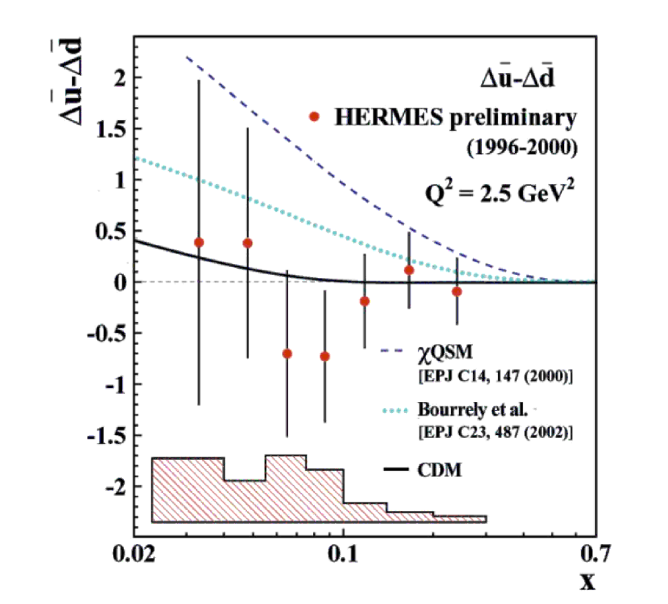
Figure 1: Flavor asymmetry of polarized sea in various models, compared with preliminary data from HERMES. The error bars indicate statistical errors, while the shaded band refers to systematic uncertainties. Adapted from Fig. 4 of Ref.[3].

As mentioned earlier, the helicity densities have been also computed in the chiral quark soliton model (CQSM) [11, 12, 13]. This model describes the nucleon as a state of $N_{c}$ valence quarks bound by a self-consistent hedgehog-like pion field. In the large-$N_{c}$ limit the distribution functions are calculated by a $1/N_{c}$ expansion. A clearcut prediction of the CQSM is that the isovector polarized antiquark distribution $\Delta\bar{f}_{-}$ is a leading quantity compared to the isoscalar distribution $\Delta\bar{f}_{+}$ and to the isovector unpolarized distribution $\bar{f}_{-}$, which both vanish at lowest order in $1/N_{c}$. Thus, one has in the CQSM

$$\frac{|\Delta\bar{f}_{-}|}{|\Delta\bar{f}_{+}|}\sim N_{c}\gg 1\,,\;\;\;\;\frac{|\Delta\bar{f}_{-}|}{|\bar{f}_{-}|}\sim N_{c}\gg 1\,,$$ (9)

and $|\Delta\bar{f}_{-}|$ is expected to be large. These behaviors are a direct consequence of the $1/N_{c}$ expansion and do not depend on the approximations used to calculate the distributions. The values of the two ratios (9) can be read out from the results presented in [13] and [12], respectively. The order of magnitude is (the spread corresponds to the variation over the experimentally accessible $x$ range)

$$\frac{\Delta\bar{u}-\Delta\bar{d}}{\Delta\bar{u}+\Delta\bar{d}}\sim 2-3\,,\;\;\;\;\frac{\Delta\bar{u}-\Delta\bar{d}}{\bar{d}-\bar{u}}\sim 3-4\,$$ (10)

The differences between the CDM and the CQSM predictions are therefore very large and can be fully appreciated in Fig. 1. The observables plotted in the three figures are extremely sensitive to the model used for computing them, and their accurate experimental determination would allow a definite test of the theory.

Figure 2: Ratio of polarized to unpolarized isovector antiquark distributions computed in the CDM model and compared with the ratio obtained from HERMES preliminary results and the CTEQ5LO parametrization.

Figure 3: Ratio of isovector to isoscalar polarized sea distributions computed in the CDM model, at the scale of the model (dashed line) and evolved to $Q^{2}=2.5$ GeV² (solid line).

Let us take a look at the available data. The quantity measured by HERMES is the semi-inclusive cross section asymmetry $A_{1}^{h}$. In leading-order QCD and under the assumption that the transverse spin structure function $g_{2}$ vanishes, $A_{1}^{h}$ reads

$$A_{1}^{h}(x,Q^{2})=\frac{1+R(x,Q^{2})}{1+\gamma^{2}}\,\frac{\sum_{f}e_{f}^{2}\Delta f(x,Q^{2})\int D_{f}^{h}(z,Q^{2})\,{\rm d}z}{\sum_{f}e_{f}^{2}f(x,Q^{2})\int D_{f}^{h}(z,Q^{2})\,{\rm d}z}\,.$$ (11)

Here $R=\sigma_{L}/\sigma_{T}$ is the longitudinal to transverse photo-absorption cross section ratio, $\gamma=2m_{N}x/Q$, and $D_{f}^{h}$ are the fragmentation functions of flavor $f$ into an hadron $h$ carrying a fraction $z$ of the initial quark momentum. By combining data on hydrogen and deuterium targets and detecting final state pions and kaons in the range $0.2<z<0.8$, HERMES extracted separately $\Delta u$, $\Delta\bar{u}$, $\Delta d$, $\Delta\bar{d}$ and $\Delta s+\Delta\bar{s}$. As shown in Fig. 1, the isovector antiquark distribution $\Delta\bar{f}_{-}=\Delta\bar{u}-\Delta\bar{d}$ is found to be small and compatible with zero. This is still a preliminary result, affected by significant statistical and systematic errors, but it is reproduced reasonably well by our model (see Fig. 1). On the contrary, the large value of $\Delta\bar{f}_{-}$ predicted by the CQSM (dashed curve in Fig. 1) seems to be discarded by the data (the dotted curve is the prediction of the statistical model of Bourrely et al. [14], that we do not discuss here). In Fig. 2 we divided the HERMES data by the unpolarized asymmetry $\bar{d}-\bar{u}$ as given by the CTEQ5LO parameterization [15], which is essentially driven by the Drell-Yan data. We attributed to the CTEQ5LO fit an absolute uncertainty of $\sim 10\%$ in the relevant range of $x$, mimicking in this way the Drell-Yan errors. The resulting points are plotted with the propagated errors and the total error bars are dominated by the large uncertainties on $\Delta\bar{u}-\Delta\bar{d}$. Once more, the agreement with the CDM prediction (solid line) is fairly good, while the high CQSM values seem to be excluded.

4. Before coming to the conclusions, we would like to comment on some technicalities concerning the model calculation of antiquark densities. Let us first notice that, if we adhere to the definition (5) of quark distributions, the variable $x=k^{+}/p^{+}$ (where $k^{+}$ is the light-cone quark momentum) is not constrained a priori to be positive. It turns out that there is a relation connecting quark and antiquark distributions, which are obtained by continuing $x$ to negative values. For helicity distributions this relation is

$$\Delta\bar{f}(x)=\Delta f(-x)\,.$$ (12)

In some approaches, including that of [11, 12, 13], the antiquark distributions are computed by means of (12). This is, in principle, an unsafe procedure. The reason is that there are semi-connected diagrams that contribute to the distributions for $x<0$, whereas in computing these distributions in the physical region only connected diagrams should be considered (indeed, this defines the parton model, as pointed out by Jaffe [16]). Our approach has no such problem: the antiquark distributions are calculated directly from their field-theoretical expression (6), by inserting a complete set of intermediate states, as explained above. Incidentally, we notice that the different techniques adopted for computing the antiquark distributions are probably at the origin of the sign discrepancy between the transversity sea distributions computed in [9] and in [13].

5. In summary, we showed that the chiral chromodielectric model and the chiral quark soliton model predict very different behaviors for the polarized isovector distribution $\Delta\bar{f}_{-}$ and for the ratios of $\Delta\bar{f}_{-}$ to the unpolarized isovector distribution, $\Delta\bar{f}_{-}/\bar{f}_{-}$, and to the polarized isoscalar distribution, $\Delta\bar{f}_{-}/\Delta\bar{f}_{+}$. The recent preliminary HERMES data favor the CDM results and exclude the large value for $\Delta\bar{f}_{-}$ predicted by the CQSM. Hopefully, more precise data in the next future will say a conclusive word about the whole question.

It is a pleasure to thank Paola Ferretti Dalpiaz for various useful discussions.

References

- [1] J. Ashman et al. (EMC), Phys. Lett. B206 (1988) 364.
-
[2]
M. Anselmino, A. Efremov and E. Leader, Phys. Rep. 261 (1995) 1.
B. Lampe and E. Reya, Phys. Rep. 332 (2000) 1.
B.W. Filippone and X.-D. Ji, Adv. Nucl. Phys. 26 (2001) 1. - [3] M. Beckmann (HERMES), hep-ex/0210049.
- [4] A.W. Schreiber, A.I. Signal and A.W. Thomas, Phys. Rev. D44 (1991) 2653.
- [5] V. Barone and A. Drago, Nucl. Phys. A552 (1993) 479; ibid. A560 (1993) 1076 (E).
- [6] V. Barone, A. Drago and M. Fiolhais, Phys. Lett. B338 (1994) 433.
-
[7]
H.J. Pirner, Prog. Part. Nucl. Phys. 29 (1992) 33.
M.C. Birse, Prog. Part. Nucl. Phys. 25 (1990) 1.
M.K. Banerjee, Prog. Part. Nucl. Phys. 31 (1993) 77. - [8] T. Neuber, M. Fiolhais, K. Goeke and J.N. Urbano, Nucl. Phys. A560 (1993) 909.
- [9] V. Barone, T. Calarco, A. Drago, Phys. Lett. B390 (1997) 287.
- [10] J. Soffer, Phys. Rev. Lett. 74 (1995) 1292.
- [11] D.I. Diakonov et al., Nucl. Phys. B480 (1996) 341; id., Phys. Rev. D56 (1997) 4069.
- [12] B. Dressler et al., Eur. Phys. J. C14 (2000) 147.
- [13] M. Wakamatsu and T. Kubota, Phys. Rev. D60 (1999) 034020.
- [14] C. Bourrely et al., Eur. Phys. J. C23 (2002) 487.
- [15] H.L. Lai et al. (CTEQ), Eur. Phys. J. C12 (2000) 375.
- [16] R.L. Jaffe, Nucl. Phys. B229 (1983) 205.