SLAC-PUB-10005 June 2003

Flavor Constraints on Split Fermion Models

Ben Lillie and JoAnne L. Hewett

Stanford Linear Accelerator Center

Stanford CA 94309, USA

We examine the contributions to rare processes that arise in models where the Standard Model fermions are localized at distinct points in compact extra dimensions. Tree-level flavor changing neutral current interactions for the Kaluza-Klein (KK) gauge field excitations are induced in such models, and hence strong constraints are thought to exist on the size of the additional dimensions. We find a general parameterization of the model which does not depend on any specific fermion geography and show that typical values of the parameters can reproduce the fermion hierarchy pattern. Using this parameterization, we reexamine the contributions to neutral meson mixing, rare meson decays, and single top-quark production in $e^{+}e^{-}$ collisions. We find that it is possible to evade the stringent bounds for natural regions of the parameters, while retaining finite separations between the fermion fields and without introducing a new hierarchy. The resulting limits on the size of the compact dimension can be as low as  TeV^-1.

1 Introduction

In recent years there has been much interest in the possibility that there may exist compact extra dimensions with sizes far above the Planck length. In particular, the possibility of $\,{\rm TeV}^{-1}$-sized extra dimension arises in braneworld theories [1, 2, 3, 4, 5, 6]. By themselves, they do not allow for a reformulation of the hierarchy problem, but they may be incorporated into a larger structure in which this problem is solved, such as the case of large extra dimensions [7, 8, 9]. In the scenario with $\,{\rm TeV}^{-1}$ extra dimensions, the Standard Model (SM) fields are phenomenologically allowed to propagate in the bulk. These models are hence subject to stronger experimental constraints and have distinct experimental signatures from the case where gravity alone is in the bulk.

There are many possibilities for how to place the Standard Model fields in the $\,{\rm TeV}^{-1}$ bulk. In the universal extra dimensions scenario all fields see the extra dimensions, giving rise to a conserved parity that relaxes direct production and precision electroweak constraints, and may provide a dark matter candidate [10, 11, 12, 13]. The effects of universal extra dimensions in rare processes have been considered in [14, 15, 16, 17]. It is also possible to localize the fermions without localizing the bosons, which allows for the gauge fields to propagate freely throughout the bulk. More recently it was noticed by Arkani-Hamed and Schmaltz (AS) that one could localize different fermion species at different points in the $\,{\rm TeV}^{-1}$ extra dimensions [18]. These “split fermion” models naturally suppress many dangerous operators, particularly those inducing proton decay. They also can naturally generate large Yukawa hierarchies; and it has been shown by multiple authors that there exist models which can generate the correct spectrum of fermion masses, as well as the correct magnitudes for CKM matrix elements [19, 20, 21, 22, 23, 24]. The most stringent generic limits in this case arise from precision electroweak measurements, which place the compactification radius at $R\lesssim 2-4\,{\rm TeV}^{-1}$ [25, 26, 27, 28]. The specific fermion locations can be probed in high energy collisions, and at very large energies, cross sections will rapidly vanish since split fermions will completely miss each other in the extra dimensions.[29, 30]

This makes the split fermion scenario an attractive possibility for the origin of the Yukawa hierarchy. However, split fermions (like most models of the fermion spectrum) are also capable of generating large flavor changing neutral currents (FCNC). The magnitude of these currents in the neutral meson sector has been estimated by several groups, and apparently generate strong constraints[21, 31, 32]. In this paper we reexamine these computations to derive more model independent constraints on split fermion models arising from FCNC and show that it is possible to evade the stringent bounds for natural regions of the parameters.

This paper is organized as follows. In Section 2 we set up the split fermion scenario in as much generality as possible and give statistical arguments to demonstrate that they can account for the observed fermion spectrum. We then describe how FCNC are generated in this scenario. In section 3 we calculate the effects on neutral meson oscillation. Section 4 presents the effects on rare $B$ decays, and single top production in $e^{+}e^{-}$ collisions, and Section 5 concludes.

2 The Model of Split Fermions

Here, we construct a very general model that characterizes the effects of separating the Standard Model fermions in an extra dimension. We start by examining the original model considered by AS.

In the AS model there is one extra dimension, which is taken to be flat. It is possible that this extra dimension is actually a “brane” with a finite width embedded in some other extra-dimensional scenario. For this reason $\,{\rm TeV}^{-1}$ dimensions are often called “fat branes”, but they need not be tied to other models. Note that if the brane is not a string theory object, but arises from some field theory mechanism, then it necessarily has finite extent in the extra dimensions. This makes the study of fat branes essential to building realistic field-theoretic models of extra dimensional scenarios.

In this model the Standard Model fields are localized to the brane. Note that the word brane here refers to any mechanism for achieving this localization. It may or may not be the same as the branes encountered in string theory. Initially, all fields are allowed to propagate in the entire dimension. In addition to the fields present in the Standard Model, there is a real scalar field which couples to the fermions, but not to the gauge bosons or the Higgs.

If the scalar has a $Z_{2}$-symmetric potential, then it can develop a stable solution which tunnels from one of the vacua to the other, called a kink solution. A mechanism for localizing fermions to a thin but finite width region inside a domain wall has been known for some time [33]. There it was noted that in 1+1 dimensions a massless fermion with a Yukawa coupling to a scalar field that has a kink-profile vacuum expectation will develop a zero mode, with a Gaussian profile centered at the location of the kink. This can be trivially extended to more dimensions by considering a domain wall instead of a soliton and making all zero modes constant in the transverse directions. Note that a five-dimensional fermion field contains two four-dimensional fermions, one of each chirality. If the extra dimension is infinite, then the zero-mode of only one chirality is normalizable. If the extra dimension is finite then something else is needed to produce chirality. A standard procedure is to compactify the dimension on an $S^{1}/Z_{2}$ orbifold, which projects out the unwanted chirality. A nice side-effect of this is to render the kink absolutely stable.

In contrast to the fermion sector, the gauge bosons are free to propagate throughout the extra dimension. Since the dimension is compact, and flat, the mass spectrum of the Kaluza-Klein gauge states is linear with $M_{n}^{2}=n^{2}/R^{2}$, and the orbifold boundary conditions project out the odd solutions, so the wavefunctions along the fifth dimension, $y$ where $0\leq y\leq R$, are

$$A^{(n)\mu}(x,y)=\sqrt{\frac{2}{R}}\cos(\frac{n\pi y}{R})A^{\mu}(x)\hskip 28.45274pt(n\geq 1),$$ (1)

where $R$ is the size of the extra dimension. Putting all this together allows investigation of brane world models where there is a single extra-dimension of roughly inverse $\,{\rm TeV}$ size with fermions localized in the center and gauge bosons propagating though the entirety.

A more interesting picture can be obtained by thinking about the fermion localization mechanism. There is a simple heuristic for why this should occur. The fermion is Yukawa coupled to a scalar field which develops a non-zero VEV. The ordinary fermion Higgs phenomena should then give the fermion a mass. However, the VEV is position dependent and in particular there is a place where it is zero (the center of the kink). So the fermion has a position dependent mass, which is somewhere zero. Thus, the fermion is easiest to excite near the zero mass, and so most of the probability for the lowest lying state (the zero mode) will live near the center of the kink.

Given that heuristic, it should be reasonable that if the 5D fermion has a mass $M$, then the center of the Gaussian moves to $y=M/2\mu^{2}$, where $\mu$ is the slope of the kink profile, and $v$ is the scale of the VEV. Indeed, it turns out that this is the case, as was first noted by Arkani-Hamed and Schmaltz [18]. This allows different fermion fields to be localized at different points in the extra dimension. To see why this is desirable, consider an operator, $\cal O$, that involves fermions separated by a distance $d$. The effective 4D coupling in the dimensionally reduced theory is proportional to the integral over the extra dimensions of the wavefunctions of all fields appearing in $\cal O$. Since the fermion wavefunctions are Gaussian, this gives a suppression proportional to $e^{-a\mu^{2}d^{2}}$, where $a$ depends on the operator being considered. This has been shown to be very effective at suppressing dangerous higher-dimensional operators, such as proton decay. Additionally, the fact that exponentially different couplings can result from linear separations provides a natural means of explaining the fermion mass hierarchy. Lighter fermions have greater separation between their left and right handed components. In this way Arkani-Hamed and Schmaltz proposed a theory to explain the Yukawa hierarchy without invoking new symmetries, and which is safe from proton decay. Several authors have proposed specific “geographies” that do indeed reproduce the correct fermion masses, as well as the CKM parameters [19, 20, 21].

There are, however, other potentially dangerous effects of the fermion separation which are not suppressed by this mechanism. The gauge bosons will have a Kaluza-Klein (KK) tower of states. The zero modes, which are flat in the extra dimensions, correspond to the SM gauge fields, and have the correct couplings to the fermion zero modes. On the other hand, the excited states have cosine profiles, as given in Eq. (1). The coupling strength of these modes to the fermions are scaled by an integral over the overlap of the fermion and gauge wavefunctions. However, since the height of the boson wavefunction will be different at the locations of the different fermions, there will be non-universal couplings of a single gauge KK-state to different fermion species. This leads to the possibility of flavor changing interactions, including tree-level neutral currents, for the KK-modes of the $\gamma$, $Z$, and gluon, as illustrated in Fig 1. One then expects large effects to come from the tree-level contributions of the KK gluon states to FCNC processes, in particular to neutral meson oscillation. Calculation of these effects can put limits on the size of the extra dimension. Also, note that while this discussion was motivated by the kink model, these issues will be relevant to any model with split fermions. This is an example of the general principle that any attempt to explain the Yukawa hierarchy will necessarily treat flavors differently, and will tend to generate large flavor-changing effects.

Figure 1: Feynman diagram for the tree-level KK gauge exchange mediating neutral meson oscillation.

In practice, geography independent constraints have been difficult to obtain due to the large number of parameters in the model. These are, $R$, $\sigma$, the width of the fermion wavefunctions (which is $1/\mu$ in the kink model), and $(d^{n}-d)$ positions, where $d$ is the number of extra dimensions and $n$ is the number of independent fermion fields. Previous discussions [21, 31, 32] have put constraints on $R$ only by first obtaining a single set of positions that reproduce the Yukawa couplings of the Standard Model, and calculating the flavor-changing effects in that particular geography. However, one would like a more model-independent way of understanding the magnitude of flavor effects in this class of models.

To accomplish this we consider the problem of FCNC in split fermion models in as much generality as possible. A specific, realistic model exists in string theory [32], as well as the field theory example just presented. In summary, we abstract from these the following points:

1. There exist one or more extra dimensions, compactified with a radius $R$.

2. Each fermion field, $\psi_{i}$ has a chiral zero mode that is localized near the center of the dimension at $y_{i}$, with Gaussian profiles $\psi\sim e^{-(y-y_{i})^{2}/\sigma^{2}}$, where the width $\sigma\ll R$. If there is more than one extra dimension they are taken to be isotropic in those dimensions $\psi\sim e^{-(\vec{y}-\vec{y_{i}})^{2}/\sigma^{2}}$.

3. The gauge bosons are free to propagate in the entire “fat brane” part of the extra dimension. (There may be a larger bulk accessible to gravity.)

4. The boundary conditions for the bosons are taken to be such that the wavefunction for the $n$-th KK-mode is $A\sim\cos(n\pi y/R)$. Note that these are generally the same conditions that allow chiral zero modes for the fermions.

5. The field content (gauge group, number and charge of matter fields) is identical to the Standard Model, plus whatever fields are necessary to localize the fermions.

These assumptions generate an effective four-dimensional Lagrangian that reduces to the Standard Model at low energies. The new features present are the propagating gauge KK-modes, their couplings, and the fact that the Higgs Yukawa couplings are determined by the fermion locations.

We now construct the interaction Lagrangian for this scenario, focusing on the quark sector in this paper. An analogous treatment of the leptonic sector can be performed. Note that there are excited states of the fermion fields in addition to the KK boson states. However, since the fermions are localized with a width smaller than R, the scale of the fermion excitations will be significantly higher than that of the KK gauge states. In addition, the fermion KK modes do not participate in the processes considered here. We therefore only consider the fermion zero modes, while we include the complete KK-tower for the bosons. With one extra dimension the coupling of the $n$-th KK boson to a flavor localized at the scaled position $\ell=x/R$ is determined by the overlap of wavefunctions

$$\int_{0}^{1}dy\bar{\psi}(y)\psi(y)A^{(n)}(y)\simeq\int_{0}^{1}dy\cos\left(n\pi y\right)e^{-(y-\ell)^{2}R^{2}/\sigma^{2}}\simeq\cos\left(n\pi\ell\right)e^{-n^{2}\sigma^{2}/R^{2}}.$$ (2)

where y has now been normalized to R. For $\delta$ extra $\,{\rm TeV}^{-1}$ dimensions this generalizes to

$$c^{(\vec{n})}(\ell)\equiv\left(\prod_{k=1}^{\delta}\cos\left(n_{k}\pi\ell_{k}\right)\right)e^{-{\vec{n}}^{2}\sigma^{2}/R^{2}}.$$ (3)

The gauge coupling of the gluons, for instance, can then be written in flavor space as

$${\cal L}_{\rm int}=\sqrt{2}g_{s}G_{(n)\mu}^{A}\left(\bar{\bf d}_{L}\gamma^{\mu}T^{A}C^{(n)}_{L}{\bf d}_{L}+\bar{\bf d}_{R}\gamma^{\mu}T^{A}C^{(n)}_{R}{\bf d}_{R}\right)+({\bf d}\rightarrow{\bf u})+{\rm h.c.}.$$ (4)

Here ${\bf d}_{L(R)}$ is the vector of left (right) handed down-type quarks, $\bar{\bf d}=(d\ s\ b)$, $g_{s}$ is the SU(3) coupling constant, and $G^{(n)\mu}$ is the $n$-th KK gluon field. The diagonal matrices $C^{(n)}_{i}$ are the wavefunction overlaps given by Eq. (2). The factor of $\sqrt{2}$ arises from the rescaling of the gauge kinetic terms to the canonically normalized value for all $n$.

Now, the Higgs zero mode, which is the Standard Model Higgs, is flat in the extra dimension, $H^{0}\propto 1/R$. Then the Yukawa couplings to the 4D Higgs field are given by

$$R\lambda_{5}\int_{0}^{1}dyH^{0}\bar{q}_{L}q_{R}\simeq\lambda_{5}\int_{0}^{1}dy\ e^{-(y-y_{i})^{2}/\sigma^{2}}e^{-(y-y_{j})^{2}/\sigma^{2}}\simeq\lambda_{5}e^{-(y_{i}-y_{j})^{2}/\sigma^{2}}.$$ (5)

Here $\lambda_{5}$ is an overall 5D coupling constant that is fixed to be ${\cal O}(1)$ by the top quark mass. We write the 4D Yukawa couplings to (for instance) the down-type quarks in the flavor basis as

$${\cal L}_{\rm Yukawa}=\bar{d}V_{R}^{(d)\dagger}M_{d}V_{L}^{(d)}d$$ (6)

Where $V_{R}^{(d)\dagger}M_{d}V_{L}^{(d)}$ is the matrix of Yukawa couplings with elements given by Eq. (5), and $M_{d}$ is the diagonal mass matrix.

We can now write the relevant terms of the Lagrangian as

$${\cal L}=\bar{\bf d}_{L}V_{R}^{(d)\dagger}M_{d}V_{L}^{(d)}{\bf d}_{R}+\bar{\bf u}_{L}V_{R}^{(u)\dagger}M_{u}V_{L}^{(u)}{\bf u}_{R}+\frac{g}{\sqrt{2}}W^{(0)}_{\mu}\bar{\bf u}_{L}\gamma^{\mu}{\bf d}_{L}$$

$$+\sum_{n=1}^{\infty}\left[\sqrt{2}g_{s}G^{(n)A}_{\mu}\left(\bar{\bf d}_{L}\gamma^{\mu}T^{A}C^{(n)}_{L}{\bf d}_{L}+\bar{\bf d}_{R}\gamma^{\mu}T^{A}C^{(n)}_{R}{\bf d}_{R}\right)+({\bf d}\rightarrow{\bf u})\right]+{\rm h.c.}$$ (7)

After the usual transformation to the mass basis, the CKM-matrix is clearly the product $V^{(u)\dagger}_{L}V^{(d)}_{L}$. Note, however, the presence of non-universal couplings prevents the products $U^{q(n)}_{i}\equiv V^{(q)\dagger}_{i}C^{(n)}_{i}V^{(q)}_{i}$ from being trivial, so there are flavor-changing interactions in the KK-gluon sector. These also occur in the excited photon and $Z$ couplings. However, those are suppressed relative to the gluons by a factor of $g/g_{s}$, so we expect that the KK-gluons will dominate any process to which they contribute.

Before examining the numerical impact of the tree-level FCNC interaction in rare processes, it will first be useful to get a handle on how far the fermions need to be separated. It has been shown by Grossman and Perez [19] that there exists at least one set of positions that correctly reproduces the observed fermion spectrum and magnitude of the CKM elements. They found that, subject to a certain set of naturalness assumptions, there was a single solution. A different solution was found in [21] by choosing different up and down-type Yukawa coupling constants in the 5D theory. Typical separations in these solutions are from $1-20$ units of the fermion width. In what follows, we parameterize the separation between 2 fermions in units of the width, i.e. $\Delta y=y_{i}-y_{j}=\alpha_{ij}\sigma$, and treat $\alpha_{ij}$ as phenomenological parameters. In addition, we find it useful to define $\rho=\sigma/R$.

As a counterpoint to the studies in [19] and [21] we have performed a simple Monte-Carlo analysis in an attempt to see how large of a hierarchy is generated naturally for fermions randomly distributed on an interval. To do this we randomly draw fermion positions from a distribution flat on the interval $[0,\alpha_{\rm max}]$, and use these to compute the Yukawa matrices from Eq. (5). We then compute the singular values of these matrices, which are the fermion masses. We can get a sense of the hierarchy by taking a particular Yukawa matrix (say the up-type) and finding the ratio of the largest to smallest singular value. In Fig 2 we show a histogram of the log of this ratio for $\alpha_{\rm max}=15$. For comparison we have computed the same value for a “null hypothesis” where instead of the split fermion scenario, the entries of the Yukawa matrices themselves are drawn directly from a distribution flat on the interval $[0,1]$. As expected, the case of split fermions clearly generates a much larger hierarchy. What is surprising is that one needs to set $\alpha_{\rm max}\approx 10-15$ before a hierarchy of six orders of magnitude becomes common, while in [18] it was claimed this hierarchy could result from $\alpha_{\rm max}\approx 5$. The discrepancy is due to the fact that, while a separation of $\alpha=5$ will indeed generate a matrix element of order $10^{-6}$, the singular values (which are the actual masses) of a full Yukawa matrix with separations no larger than 5 will tend to be too large. We note that the full fermion spectrum can be generated by $\rho$ as large as $1/15$, i.e. without introducing a new large hierarchy between the compactification and fermion localization scales. Also note that $\alpha_{\rm max}$ represents the part of the extra dimension in which the fermions can be localized and need not be the same as $1/\rho$, which is the size of the dimension through which the gauge bosons can propagate.

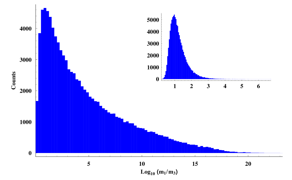
Figure 2: Histograms of $10^{5}$ random trials of the size of the fermion hierarchy, $\log(m_{1}/m_{3})$, where $m_{1}$ is the largest and $m_{3}$ the smallest mass for a single Yukawa matrix. Main graph: In the split fermion model where the positions are randomly drawn on the interval $[0,15]$ in units of the fermion width. Inset: In a “null hypothesis” where the Yukawa matrix elements are randomly drawn from the interval $[0,1]$.

3 Constraints from Neutral Meson Oscillation

Significant effects from the flavor-changing gluonic couplings should show up in neutral meson oscillations. We start by examining the effects on Kaon mixing. The $\Delta S=2$ effective Lagrangian from the single KK-gluon exchange depicted in Fig. 1 is

$${\cal L}_{\rm eff}^{\Delta S=2}=\frac{2}{3}g_{s}^{2}\sum_{\vec{n}=1}^{\infty}\frac{1}{M_{n}^{2}}\sum_{i,j=L,R}U_{i(sd)}^{d(n)*}U_{j(ds)}^{d(n)}\bar{d}_{i}\gamma^{\mu}s_{i}\bar{d}_{j}\gamma_{\mu}s_{j}$$

$$=\frac{2}{3}g_{s}^{2}\left(\vphantom{\frac{1}{2}}\right.\sum_{i,j=L,R}V^{d}_{i(11)}V^{d*}_{i(12)}V^{d*}_{j(11)}V^{d}_{j(12)}$$

$$\times\left.\vphantom{\frac{1}{2}}\times\sum_{n=1}^{\infty}\frac{(\cos(n\pi x_{d_{i}})-\cos(n\pi x_{s_{i}}))(\cos(n\pi x_{d_{j}})-\cos(n\pi x_{s_{j}}))}{M_{n}^{2}}e^{-\rho^{2}n^{2}}\right).$$ (8)

Here, the $x_{i}$ are the positions of the $d$ quark fields, $y_{i}$ of the $s$ quark, and we have used the unitarity of the $V$’s (here, we have approximated this with $2\times 2$ unitarity, we discuss the third-generation effects below). We are especially interested in the form of the sum over the KK-modes. While KK-sums are usually divergent in more than one extra dimension and require a cutoff, ours contains a natural cutoff arising from the finite width of the fermion zero mode, and hence is convergent for a number of extra dimensions $\delta\geq 1$. This is simple to understand physically. The cutoff sets in when the wavelength of the KK-mode is of order the fermion width, which occurs at $R/n_{\rm max}=\sigma$. At higher momenta the wavefunction of the boson is oscillating many times within the fermion allowing it to resolve the fermion’s wavefunction, and exponentially decouples. The fact that this cutoff arises naturally in the field theory model is an attractive feature of that particular mechanism for fermion localization.

In one additional dimension the sum converges even without the exponential suppression. In this case it is insensitive to the value of $\rho$ and can be computed analytically by ignoring the exponential factor. To do this we need to evaluate

$$F(x,y)\equiv\sum_{n=1}^{\infty}\frac{(\cos(n\pi x)-\cos(n\pi y))^{2}}{n^{2}},$$ (9)

and

$$G(x,y)\equiv\sum_{n=1}^{\infty}\frac{(\cos(n\pi x_{1})-\cos(n\pi y_{1}))(\cos(n\pi x_{2})-\cos(n\pi y_{2}))}{n^{2}}.$$ (10)

The computations for these sums are presented in the appendix. The final result is

$$F(x,y)=\frac{\pi^{2}}{2}|x-y|,$$ (11)

and

$$G(x_{1},y_{1},x_{2},y_{2})=\frac{\pi^{2}}{2}(|x_{1}-x_{2}|+|y_{1}-y_{2}|-|x_{1}-y_{2}|-|x_{2}-y_{1}|).$$ (12)

This tells us that the flavor changing effects depend, as expected, on any nonzero separation between fermion fields.

The hadronic matrix elements for the gluonic contributions to Kaon mixing are given by (computed in the vacuum insertion approximation)[35]:

$$\langle\bar{K}^{0}|\bar{d}_{L}\gamma^{\mu}s_{L}\bar{d}_{L}\gamma_{\mu}s_{L}|K^{0}\rangle =\frac{1}{3}f_{K}^{2}m_{k}$$ (13)

$$\langle\bar{K}^{0}|\bar{d}_{L}\gamma^{\mu}s_{L}\bar{d}_{R}\gamma_{\mu}s_{R}|K^{0}\rangle =f_{K}^{2}m_{k}\left(\frac{1}{12}+\frac{1}{4}\left(\frac{m_{K}^{2}}{m_{d}^{2}+m_{s}^{2}}\right)\right)$$

as well as those with $(L\leftrightarrow R)$, which have the same evaluation. Written out in full, the contribution to $\Delta m_{K}$ is then

$$\Delta m_{K}= {\cal R\mskip-4.0mu\lower 0.43057pt\hbox{\it e}\,}\langle\bar{K}^{0}|{\cal L}^{\Delta S=2}|K^{0}\rangle$$

$$=\frac{2}{3}g_{s}^{2}R^{2} \left(\vphantom{\frac{1}{1}}\right.|V^{d}_{L\ 11}V^{d*}_{L\ 12}|^{2}F(x_{d_{L}},x_{s_{L}})\langle\bar{K}^{0}|\bar{d}_{L}\gamma^{\mu}s_{L}\bar{d}_{L}\gamma_{\mu}s_{L}|K^{0}\rangle$$

$$+|V^{d}_{R\ 11}V^{d*}_{R\ 12}|^{2}F(x_{s_{R}},x_{s_{R}})\langle\bar{K}^{0}|\bar{d}_{R}\gamma^{\mu}s_{R}\bar{d}_{R}\gamma_{\mu}s_{R}|K^{0}\rangle$$ (14)

$$+(V^{d}_{L\ 11}V^{d*}_{L\ 12}V^{d*}_{R\ 11}V^{d}_{R\ 12})G(x_{d_{L}},x_{s_{L}},x_{d_{R}},x_{s_{R}})\langle\bar{K}^{0}|\bar{d}_{L}\gamma^{\mu}s_{L}\bar{d}_{R}\gamma_{\mu}s_{R}|K^{0}\rangle$$

$$+(V^{d}_{R\ 11}V^{*d}_{R\ 12}V^{*d}_{L\ 11}V^{d}_{L\ 12})G(x_{d_{L}},x_{s_{L}},x_{d_{R}},x_{s_{R}})\langle\bar{K}^{0}|\bar{d}_{R}\gamma^{\mu}s_{R}\bar{d}_{L}\gamma_{\mu}s_{L}|K^{0}\rangle\left.\vphantom{\frac{1}{1}}\right),$$

where $x_{d_{L,R}}$ are the positions of the $d$ field, and the $x_{s_{L,R}}$ of the $s$. Note that all possible separations (between quark fields) are present, but some enter with different signs. In principle then, the gluonic contribution could be made small for any values of $R$ and $\rho$ by placing the quarks at appropriate places. However, the terms involving only right or left handed fields occur with the same sign. So, to achieve significant reduction, cancellations must occur between those terms and the terms which involve both chiralities. This involves tuning the quark positions to the values of different hadronic matrix elements, which introduces a fine-tuning problem. Otherwise, it would imply that the UV physics that localizes the quarks has information about the IR behavior of QCD! We can therefore expect that cancellations will be ${\cal O}(1)$ at most. This is seen clearly in the Monte Carlo trials, where the random positions have no relation to the hadronic matrix elements and no significant cancellation occurs.

In light of this we can explore the magnitude of the flavor effects just by looking at a single term in (14); for convenience we choose the first. We can then describe the contributions with only three parameters: the radius $R$, the scale ratio $\rho$, and the separation between one pair of fermions, $\alpha$. The sum over KK-modes is then calculable in terms of these parameters. Since $R$ enters only in the mass in the KK propagator, we can write the contribution in the simple form

$$\Delta m_{K}=\frac{2}{9}g_{s}^{2}f_{K}^{2}m_{K}R^{2}V_{\rm ds,ds}^{4}F_{\rho}(\rho\alpha)$$ (15)

where $V_{ds,ds}^{4}$ stands for the appropriate product of 4 elements of the $V^{u,d}_{L,R}$ matrices, two at each vertex, and, as shown in (11), $F(x,y)$ only depends on the difference of it’s arguments, so we can write it as a function of only a single variable, given by the product $\rho\alpha$. The subscript on F reminds us that in two dimensions or more $F$ also depends on $\rho$ directly as the cutoff parameter, in which case it must be computed numerically. If we demand that this contribution to $\Delta m_{K}$ be no larger than the measured value (a conservative assumption from the point of view of constraining the model) we get

$$\frac{1}{R}\geq\beta_{K}\sqrt{V_{ds,ds}^{4}F_{\rho}(\rho\alpha)},$$ (16)

where $\beta_{K}$ is a coefficient of dimension 1, which depends on the meson parameters. This expression immediately generalizes to other neutral meson systems by using the appropriate coefficient $\beta$, and the appropriate matrix elements of $V$. Table 1 shows the values of $\beta$ for cases of interest, along with representative values of $F_{\rho}(\rho\alpha)$.

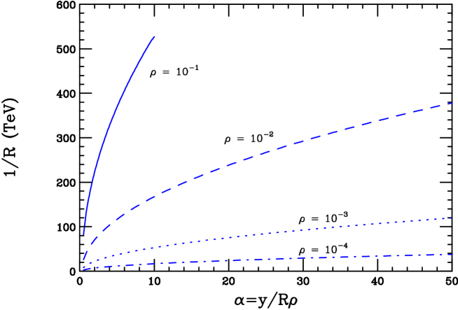
Figure 3: The behavior of the constraint on $1/R$ with $\alpha$ for various values of $\rho$. The area below the curves is excluded. Note that the size of the additional dimension in units of the fermion width is $1/\rho$, so the curve for $\rho=1/10$ ends at a maximal separation of $\alpha=10$.

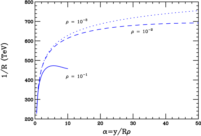
Figure 4: Constraints on $1/R$ from Kaon mixing for two extra dimensions; the area below the curves is excluded.

The resulting constraints are shown in Fig. 3 and 4, for 1 and 2 extra dimensions respectively, using the value of $\beta$ and $V_{ds,ds}^{4}$ appropriate for the Kaon sector, and assuming that the $V$ are CKM-like in magnitude (we discuss that assumption in detail below). There are two features of note. First, with one extra dimension the constraint is a simple square-root function, as can be seen from Eq. (11). This means that the flavor-changing effects can be made arbitrarily small by reducing $\rho$. That is, by increasing the hierarchy between fermion and boson scales. Second, in two dimensions the effect seems to be roughly constant in $\rho$, and flattens off at large $\alpha$. We know that the sum over the KK states is diverging logarithmically before it reaches the cutoff, and so it should be getting larger as $\rho$ decreases. However, shrinking $\rho$ brings the fermions closer together making the flavor effects smaller. In two dimensions these two effects are seen to roughly cancel. In three or more dimensions, the divergence of the sum wins completely, and the bounds on $R^{-1}$ are huge, effectively removing these cases from consideration as realistic models.

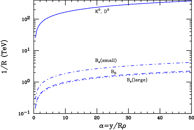
Figure 5: Constraints from all species of neutral meson mixings for one extra dimension, taking $\rho=1/100$. See text for a description of the experimental values used. Note that the $K^{0}$ and $D^{0}$ results are separate lines that overlap due to a numerical coincidence.

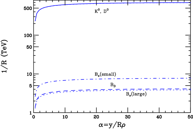
Figure 6: Neutral meson constraints for two extra dimensions. The area below the curves is excluded.

In Figs. 5 and 6 we display our results for all meson mass differences, taking $\rho=1/100$. For mixing in the Kaon sector and $B_{d}^{0}$ sector, the bound is set by demanding that the new physics produce an effect which is no larger than the observed value. For $D^{0}$ mixing, the effect is restricted to lie below the current experimental bound. There is no experimental upper bound on $B_{s}^{0}$ mixing, so we assume two values, one the size expected in the Standard Model, the other about 4 times larger, corresponding to the curves labeled small and large, respectively. Note that the most stringent constraints come from mixings involving the first and second generation.

$\rho$ $\alpha=1$ $\alpha=5$ $\alpha=10$ $\alpha=20$ $\alpha=50$ 1D $10^{-1}$ 1.15 2.33 4.76 NA NA $10^{-2}$ 0.036 0.23 0.48 1.00 2.45 $10^{-3}$ 0.0012 0.023 0.048 0.097 0.25 2D $10^{-1}$ 2.05 3.82 3.59 NA NA $10^{-2}$ 2.25 5.27 6.46 7.47 8.22 $10^{-3}$ 2.27 5.41 6.67 8.08 9.78           Meson $\beta$( MeV) $K^{0}$ 1125.86 $B^{0}_{d}$ 478.01 $B^{0}_{s}$ 67.4346 $D^{0}$ 1124.23

Table 1: Left: Representative values of the sum $F_{\rho}(\rho\alpha)$ for one and two extra dimensions. Right: Multiplicative $\beta$ factors for mass splittings of the neutral mesons; $1/R\geq\beta\sqrt{V^{4}F_{\rho}(\rho\alpha)}$.

This pattern suggests a loop-hole in the otherwise stringent constraints. Namely, the $V$ matrices need not be CKM-like. Since the CKM matrix is the product $V_{L}^{(u)\dagger}V_{L}^{(d)}$, the observed CKM hierarchical structure could result from a completely different structure at the level of the $V^{i}$. If there is small first to second generation mixing the Kaon and $D^{0}$ constraints will be relaxed, and all constraints would then be of order a few  TeV, even for large values of $\rho$.

However, in the previous calculation we ignored the third generation when imposing the unitarity condition in Eq. (8). Transitions between two 4D mass eigenstates will involve all three generations in the localization (flavor) basis. In this case the matrices $U^{(n)}_{i}$ will contain the positions of all three generations of quarks, and the unitarity conditions on the $V$ matrices will be changed. For instance, for the term in Eq. (14) with both left-handed chiralities (and dropping the $L$ index), in place of $|V^{d}_{L\ 11}V^{d*}_{L\ 12}|^{2}F(x_{d},x_{s})$ we should have

$$|V_{11}|^{2}V_{12}V^{*}_{13}F(x_{d},x_{s})+V^{*}_{11}V_{12}V^{*}_{32}V_{31}G(x_{d},x_{s},x_{b},x_{s})$$

$$+V^{*}_{31}V_{32}V^{*}_{13}V_{11}G(x_{b},x_{s},x_{d},x_{s})+|V_{31}|^{2}|V_{32}|^{2}F(x_{b},x_{s})$$ (17)

These additional terms (including the ones not displayed above corresponding to right and mixed chiralities) will insure that in any mass splitting observable many mixing angles and fermion separations will enter. It then becomes non-trivial to reduce $\Delta m_{K}$ by adjusting mixings alone. However, it is still possible to reduce the Kaon and $D^{0}$ constraints by noticing that the new terms contain fewer diagonal elements. Hence, if the weak and mass eigenbases are not too badly misaligned, i.e. the $V^{i}$ have large diagonal elements and smaller off-diagonal elements, then the strongest constraints may be relaxed somewhat. To get a better sense of what is typically possible, we again run Monte Carlo simulations. From these we learn that a typical suppression factor is $10^{-1}$ for the factors multiplying $\beta$ in Eq. (16), $10^{-2}$ is not uncommon, and $10^{-4}$ is obtainable, but rare, even for the fairly large value $\alpha_{\rm max}=15$. This is illustrated in Fig. 7.

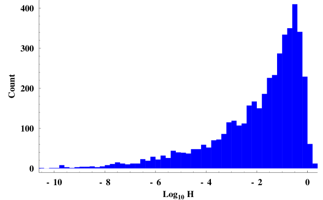
Figure 7: Histogram of values of the factor $H=\sqrt{\sum V^{4}F(x,y)}$ summed over the appropriate fermion positions and $V$ matrix elements.

All of these considerations together show that once the parameter space is thoroughly explored, it is possible to evade the large constraints from meson mixing for natural regions of the parameters.

4 Rare Decays

We also consider processes involving only a single flavor-changing vertex. The best examples of this type which receive contributions from KK gluon exchange are rare $B$ decays, such as $B\rightarrow\psi K_{S}$ and $B\rightarrow\phi K_{S}$. The most interesting aspects of these decays are, of course, their associated CP-violating asymmetries. However, since we have no control of the phases present in split fermion models, we can’t address the new contributions to CP-violating observables in a model independent fashion. Nonetheless, there are tree-level strong coupling contributions to these decays, so we can expect significant contributions to the branching fractions in split fermion models.

The effective Lagrangian for a process with a single flavor change is given by

$${\cal L}_{\rm eff}^{\Delta b=1}=\frac{2}{3}g_{s}^{2}\sum_{n=1}^{\infty}\frac{1}{M_{n}^{2}}\sum_{i,j=L,R}U_{i(qb)}^{d(n)}\bar{q}_{i}\gamma^{\mu}b_{i}\bar{q}_{j}\gamma^{\mu}q_{j}.$$ (18)

Since one vertex is flavor diagonal, the sum depends on the absolute position of the fermions. For instance, the analog of Eq3. (9-11) is

$$F^{\prime}(x,y,z) =\sum_{n=1}^{\infty}\frac{\cos(n\pi z)(\cos(n\pi x)-\cos(n\pi y))}{n^{2}}$$

$$=-\frac{\pi^{2}}{4}\left(\vphantom{\frac{1}{2}}|z+x|+|z-x|-|z+y|-|z-y|+\pi x^{2}-\pi y^{2}\right).$$ (19)

where $z$ corresponds to the location of the quark at the flavor conserving vertex. This additional complication turns out to be minor, as the actual magnitude of the sum is similar to that in the previous case and does not vary much over the parameter space, as can be seen from Fig. 8.

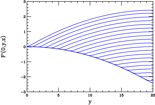
Figure 8: KK sum for processes involving a single flavor changing vertex as a function of one of the fermion positions, corresponding to the case where one of the fermions is localized at the orbifold fixed point. The position of the third (flavor conserved) fermion, $z$, is varied in steps of one unit, with $z=0$ corresponding to the top curve and $z=20$ to the bottom. The sum is done for a single extra dimension of size 20 units.

We consider the decay amplitude

$${\cal A}(B\rightarrow\phi K_{S})=\frac{2}{3}g_{s}^{2}R^{2}\sum_{i,j=L,R}F^{\prime}(x_{b_{i}},x_{s_{i}},x_{s_{j}})\langle\phi K_{S}|(\bar{s}_{i}\gamma^{\mu}b_{i})(\bar{s}_{j}\gamma_{\mu}s_{j})|B^{0}\rangle$$ (20)

The relevant matrix elements are [36]

$$\langle\phi K_{S}|(\bar{s}_{L}\gamma^{\mu}b_{L})(\bar{s}_{L}\gamma_{\mu}s_{L})|B^{0}\rangle =\frac{1}{3}H$$

$$\langle\phi K_{S}|(\bar{s}_{L,i}\gamma^{\mu}b_{L,j})(\bar{s}_{L,j}\gamma_{\mu}s_{L,i})|B^{0}\rangle =\frac{1}{3}H$$ (21)

$$\langle\phi K_{S}|(\bar{s}_{L}\gamma^{\mu}b_{L})(\bar{s}_{R}\gamma_{\mu}s_{R})|B^{0}\rangle =\frac{1}{4}H$$

$$\langle\phi K_{S}|(\bar{s}_{L,i}\gamma^{\mu}b_{L,j})(\bar{s}_{R,j}\gamma_{\mu}s_{R,i})|B^{0}\rangle =\frac{1}{12}H.$$

Here, $i,j$ are color indices, displayed explicitly in the non-singlet terms which now contribute. The common factor is

$$H=2(\epsilon_{\phi}\cdot p_{B})f_{\phi}m^{2}_{\phi}F_{+}(m_{\phi}^{2}),$$ (22)

where $\epsilon_{\phi}$ represents the polarization vector of the phi meson, and $F_{+}(q^{2})$ is the form factor for this decay. There are an additional four matrix elements obtained by taking $(L\leftrightarrow R)$. We use the values $f_{\phi}=233\,{\rm MeV}$ [37], $F_{+}(m_{\phi}^{2})=0.38$ [38], and $m_{\phi}=1020\,{\rm MeV}$ [39].

For the branching fraction we obtain (ignoring the O(1) differences among matrix elements)

$${\cal B}(B\rightarrow\phi K_{S}) =\frac{1}{64\pi m_{B}\Gamma_{B}}f_{\phi}^{2}m_{\phi}^{4}F_{+}^{2}(m_{\phi}^{2})\left(\sum_{n=1}^{\infty}\frac{U^{d\dagger}_{L(ss)}U^{d}_{L(bs)}}{n^{2}}\right)^{2}$$ (23)

$$\approx 9.1\times 10^{-6}\left(\frac{V_{sb,ss}^{4}}{0.04}\right)^{2}\left(\frac{R}{1\,{\rm TeV}^{-1}}\right)^{4}\left(\sum_{i,j=L,R}F^{\prime}(x_{b_{i}},x_{s_{i}},x_{s_{j}})\right)^{2},$$

and similarly

$${\cal B}(B\rightarrow\psi K_{S})\approx 5.6\times 10^{-5}\left(\frac{V_{sb,cc}^{4}}{0.04}\right)^{2}\left(\frac{R}{1\,{\rm TeV}^{-1}}\right)^{4}\left(\sum_{i,j=L,R}F^{\prime}(x_{b_{i}},x_{s_{i}},x_{c_{j}})\right)^{2}.$$ (24)

Demanding that this not be larger than the observed rate gives the approximate constraints $1/R\geq 1.0\ \,{\rm TeV}$ from $B\rightarrow\phi K_{S}$ and $1/R\geq 0.5\ \,{\rm TeV}$ from $B\rightarrow\psi K_{S}$. These are not competitive with those from $B_{d}$ and $B_{s}$ meson oscillation, and provide a good consistency check. It is interesting to note that if a way can be found to reduce the constraints from the Kaon sector to the few  TeV scale without disturbing the $b$-quark couplings (say by arranging the mixing angles), then this contribution to $B\rightarrow\psi K_{S},\phi K_{S}$ is of roughly the same order as that of the Standard Model. Any new phases in this scenario will thus contribute to the CP-violating observables with equal effects in each decay channel.

We have also estimated the ree-level KK contribution to single top quark production at LEP, $e^{+}e^{-}\rightarrow\bar{t}q+t\bar{q}$ (with $q=u,c$) which proceeds via KK $\gamma^{(n)}$ and $Z^{(n)}$ exchange. Using the parameterization in [40] we find an effective anomalous flavor-changing vector coupling $v_{Z}$ given in this case by

$$v_{Z{\rm eff}} =\left(\sqrt{2}+2\sin\theta_{W}Q\right)M_{W}^{2}R^{2}\sum_{i,j=L,R}\sum_{n=1}^{\infty}\frac{U^{u}_{i(tc)}U^{l}_{j(ee)}}{n^{2}}$$ (25)

$$\approx 6.9\times 10^{-4}\left(\frac{R}{1\,{\rm TeV}^{-1}}\right)^{2}\sum_{i,j=L,R}\left(\frac{V_{ut,ee}^{4}}{0.04}\right)\left(\sum_{i,j=L,R}F^{\prime}(x_{c_{i}},x_{t_{i}},x_{e_{j}})\right),$$ (26)

where we have used only the $c\rightarrow t$ since it dominates the $u\rightarrow t$ by a factor of 10. The current constraint on this effective flavor changing coupling from LEP data is $v_{Z}\leq 0.75$ [41], and so split fermions in the up-quark sector are not significantly constrained.

Lastly, we examine the potential gauge KK contributions to the purely leptonic decay of neutral $B$ mesons, $B^{0}_{q}\rightarrow\ell^{+}\ell^{-}$, with $q=d,s$. This process proceeds through tree-level $\gamma^{(n)}$ and $Z^{(n)}$ KK exchange, and could ,in principle, probes fermion splitting in the leptonic sector as well as in the quark sector. Here, for simplicity, we will assume that the leptonic fields are all localized at the same point in the extra dimension and will ignore any possible flavor changing leptonic interactions. The $\Delta b=1$ Lagragian describing this decay is then

$${\cal L}^{\Delta b=1}_{\rm eff}=\sum_{\alpha=\gamma,Z}2G^{2}_{\alpha}\,\sum_{\vec{n}=1}^{\infty}{\frac{1}{M_{n}^{2}}}\,\,\sum_{i=L,R}U^{d(n)}_{i(qb)}g^{b}_{i,\alpha}\bar{q}_{i}\gamma^{\mu}b_{i}\,g^{\ell}_{i,\alpha}\bar{\ell}_{i}\gamma_{\mu}\ell_{i}\,,$$ (27)

where $G_{\gamma}=e$ and $G_{Z}=g/\cos\theta_{w}$. The hadronic matrix element governing this decay is given by

$$\langle 0|g^{b}_{L,\gamma/Z}U^{d(n)}_{L}\bar{q}_{L}\gamma^{\mu}b_{L}+g^{b}_{R,\gamma/Z}U^{d(n)}_{R}\bar{q}_{R}\gamma^{\mu}b_{R}|B^{0}_{q}\rangle=if_{b}p^{\mu}_{B}[g^{b}_{L,\gamma/Z}U^{d(n)}_{L}-g^{b}_{R,\gamma/Z}U^{d(n)}_{R}]\,,$$ (28)

where $p^{\mu}_{B}$ represents the momentum of the $B^{0}$ meson. Due to parity, only the axial-vector current contributes to this matrix element. In the case of photon KK exchange, such contributions are generated when the left- and right-handed fermions are localized at separate points. Here, we will ignore this possibility and consider the case where only the $Z^{(n)}$ exchange mediates this decay. The branching fraction is then

$${\cal B}(B_{s}\rightarrow\mu^{+}\mu^{-}) = {\frac{4G_{F}^{2}M_{W}^{4}f_{B}^{2}m_{\ell}^{2}m_{B}}{\pi c_{w}^{4}}}\tau_{B}R^{4}\left[1-{\frac{4m_{\ell}^{2}}{m_{B}^{2}}}\right]^{1/2}\Big{|}\sum_{n}\frac{g^{b}_{L,Z}U^{d(n)}_{L}-g^{b}_{R,Z}U^{d(n)}_{R}}{n^{2}}\Big{|}^{2}$$ (29)

$$= 1.15\times 10^{-6}\left({\frac{R}{1\,{\rm TeV}^{-1}}}\right){\frac{V_{db,\mu\mu}^{4}}{(0.04)^{2}}}$$

$$\quad\times\Big{|}g_{L,Z}F^{\prime}(x_{b_{L}},x_{q_{L}},x_{\ell_{L}})-g_{R,Z}F^{\prime}(x_{b_{R}},x_{q_{R}},x_{\ell_{R}})\Big{|}^{2}\,,$$

where we have chosen $q=s$ and used $f_{B}=200$ MeV. The function $F^{\prime}$ is as given in Eq. (19) and has a value in the range $-2$ to $+2$ as shown in Fig. 8. Taking values of this function which maximizes the sum over the KK states, i.e., $F^{\prime}=2$, yields a value of unity for the sum, resulting in a branching fraction of $1.15\times 10^{-6}$ for $R=1\,{\rm TeV}^{-1}$. This is a significant enhancement over the Standard Model value[42] of ${\cal B}(B_{s}\rightarrow\mu^{+}\mu^{-})\simeq 4.0\times 10^{-9}$. The experimental bound on this decay, ${\cal B}(B_{s}\rightarrow\mu^{+}\mu^{-})<2.6\times 10^{-6}$, as determined by CDF[43], sets the limit $R^{-1}>815$ GeV when the sum over the KK states takes on its maximal value. The sensitivity of this decay mode in probing the size of the additional dimension is thus comparable to that of $B_{s}$ mixing and will improve with Run II data at the Tevatron[44].

5 Conclusions

Models where the Standard Model fermions are localized at specific points along a compact extra dimension offer an attractive means for constructing the fermion mass hierarchy and suppressing dangerous operators such as proton decay. In these scenarios, the fermions obtain narrow Gaussian wavefunctions in the additional dimension with a width much smaller than the compactification scale. The fermion Yukawa couplings are then generated by the overlap of the localized wavefunctions for the left- and right-handed fermions. Lighter fermions are thus more widely separated than heavier ones.

The gauge fields are free to propagate throughout the bulk in these scenarios and their KK excitations develop tree-level flavor changing interactions which are proportional to the overlap of their wavefunctions with those of the localized fermions. Gluons, as well as the electroweak gauge bosons, then mediate flavor changing neutral current processes at dangerous levels. Previously, it was thought that the only way to avoid stringent bounds on the size of the compact dimensions was to minimize the separation of the fermion fields, thus endangering the scenario’s natural explanation of the fermion hierarchy.

In this paper, we have reinvestigated these new FCNC interactions and have performed a general, systematic, model independent analysis. Our results hold for any such model of the fermion hierarchy with specific fermion geographies. We have employed a model parameterization which contains only three parameters: the size of the extra dimension $R$, the scaled width of the localized fermion $\rho=\sigma/R$, and the fermion separation distance expressed in units of the width, $\Delta x=\alpha\sigma$. We performed a simple Monte Carlo analysis and determined that the fermion mass hierarchy can be reproduced in our parameterization for natural values of the parameters.

We then evaluated the KK gluon tree-level flavor changing contributions to neutral meson oscillations. We found that the sum over the KK states is exponentially damped for higher KK gauge states as the KK states can then resolve the finite size of the fermion wavefunction. This allows us to perform the KK sum in a scenario with more than one extra dimension. We then evaluated the constraints from Kaon mixing in the case of one extra dimension and confirmed previous results that $1/R\mathrel{\mathchoice{\lower 3.01385pt\vbox{\halign{$\matth\displaystyle\hfil#\hfil$\cr>\crcr\sim\crcr}}}{\lower 3.01385pt\vbox{\halign{$\matth\textstyle\hfil#\hfil$\cr>\crcr\sim\crcr}}}{\lower 3.01385pt\vbox{\halign{$\matth\scriptstyle\hfil#\hfil$\cr>\crcr\sim\crcr}}}{\lower 3.01385pt\vbox{\halign{$\matth\scriptscriptstyle\hfil#\hfil$\cr>\crcr\sim\crcr}}}}100$’s TeV for larger values of $\rho$ unless the separation was very small. However, the constraint shrinks to $1/R\mathrel{\mathchoice{\lower 3.01385pt\vbox{\halign{$\matth\displaystyle\hfil#\hfil$\cr>\crcr\sim\crcr}}}{\lower 3.01385pt\vbox{\halign{$\matth\textstyle\hfil#\hfil$\cr>\crcr\sim\crcr}}}{\lower 3.01385pt\vbox{\halign{$\matth\scriptstyle\hfil#\hfil$\cr>\crcr\sim\crcr}}}{\lower 3.01385pt\vbox{\halign{$\matth\scriptscriptstyle\hfil#\hfil$\cr>\crcr\sim\crcr}}}}$ few TeV for smaller values of $\rho$, even for widely separated fermions, at the expense of introducing a new hierarchy between the compactification and fermion localization scales. The constraints from $B_{d}$ and $B_{s}$ mixing were found to be much less restrictive. We also performed the evaluation for the case of two or more additional dimensions and found that the FCNC constraints were much more difficult to evade.

We next studied the dependence of our constraints on the fermion mass mixing matrices, and found that with a realignment of the matrix elements our bounds could be reduced further by factors of 10-100.

In addition, we examined the rare meson decays $B_{d}\rightarrow\psi K_{S},\phi K_{S}$, as well as single top-quark production in $e^{+}e^{-}$ collisions, and found weaker limits of the size of the extra dimension of order TeV^-1. We note that the KK gluon contributions to these rare decays are significant enough to generate interesting effects in the related CP violation observables.

In summary, we have shown that once the parameter space is systematically explored, it is possible to evade the stringent bounds from FCNC in split fermion models for natural values of the parameters and without the introduction of any additional hierarchies. Lastly, we note that the introduction of brane localized kinetic terms are known to significantly reduce the couplings of gauge KK states [45, 46] and may help to even further reduce the constraints from FCNC in these scenarios.

6 Appendix

Here we present a cute way to perform the sum over KK modes analytically in one dimension, and see that the sum is exactly linearly proportional to the separation.[47] The functions that we need are

$$F(x,y)\equiv\sum_{n=1}^{\infty}\frac{(\cos(n\pi x)-\cos(n\pi y))^{2}}{n^{2}},$$ (30)

and

$$G(x_{1},x_{2},y_{1},y_{2})\equiv\sum_{n=1}^{\infty}\frac{(\cos(n\pi x_{1})-\cos(n\pi y_{1}))(\cos(n\pi x_{2})-\cos(n\pi y_{2}))}{n^{2}}.$$ (31)

We can do both of these by evaluating

$$f(x)\equiv\sum_{n=1}^{\infty}\frac{\cos(nx)}{n^{2}}.$$ (32)

So that

$$F(x,y) =\frac{1}{2}(f(2\pi x)+f(2\pi y)+\frac{\pi^{2}}{3}-2f(\pi x+\pi y)-2f(\pi x-\pi y))$$ (33)

$$G(x_{1},x_{2},y_{1},y_{2}) =\left[\vphantom{\frac{1}{2}}f(\pi x_{1}+\pi x_{2})+f(\pi x_{1}-\pi x_{2})+f(\pi y_{1}+\pi y_{2})+f(\pi y_{1}-\pi y_{2})\right.$$

$$\left.\vphantom{\frac{1}{2}}-f(\pi x_{1}+\pi y_{2})-f(\pi x_{1}-\pi y_{2})-f(\pi y_{1}+\pi x_{2})-f(\pi y_{1}-\pi x_{2})\right]$$ (34)

Writing the $\cos(nx)$ as two exponentials and combining the sums we have

$$f(x)=\frac{1}{2}\sum_{n\neq 0}\frac{e^{inx}}{n^{2}}.$$ (35)

The function $f$ is then the solution of the differential equation

$$f^{\prime\prime}(x) =-\frac{1}{2}\sum_{n\neq 0}e^{inx}=-\frac{1}{2}\sum_{n=-\infty}^{\infty}e^{inx}+\frac{1}{2}$$ (36)

$$=-\frac{1}{2}\left(2\pi\sum_{k=-\infty}^{\infty}\delta(x-2\pi k)-1\right).$$ (37)

This is solved by

$$H(x)=-\frac{1}{2}\left(\pi|x|-\frac{x^{2}}{2}-\frac{\pi^{2}}{3}\right),$$ (38)

where $H$ is defined on the interval $[-\pi,\pi]$ and is $2\pi$-periodic for other values (this takes care of the sum over delta functions). We then have

$$f(x)=H(x)+\alpha x+\beta.$$ (39)

Looking at the original function we see that we must have $\int_{-\pi}^{\pi}f=0$ which gives $\beta=0$. Also, since $f$ is an even function $\alpha=0$.

We can then use Eq. (39) in (33) and (34) and use the physical condition that all arguments are positive to get the final result

$$F(x,y)=\frac{\pi^{2}}{2}|x-y|,$$ (40)

and

$$G(x_{1},x_{2},y_{1},y_{2})=-\frac{\pi^{2}}{4}\left(\vphantom{\frac{1}{2}}|x_{1}-x_{2}|+|y_{1}-y_{2}|-|x_{1}-y_{2}|-|y_{1}-y_{2}|\right).$$ (41)

References

- [1] I. Antoniadis, Phys. Lett. B246, 377 (1990).
- [2] J. D. Lykken, Phys. Rev. D54, 3693 (1996), hep-th/9603133.
- [3] E. Witten, Nucl. Phys. B471, 135 (1996), hep-th/9602070.
- [4] P. Horava and E. Witten, Nucl. Phys. B475, 94 (1996), hep-th/9603142.
- [5] P. Horava and E. Witten, Nucl. Phys. B460, 506 (1996), hep-th/9510209.
- [6] E. Caceres, V. S. Kaplunovsky, and I. M. Mandelberg, Nucl. Phys. B493, 73 (1997), hep-th/9606036.
- [7] N. Arkani-Hamed, S. Dimopoulos, and G. R. Dvali, Phys. Lett. B429, 263 (1998), hep-ph/9803315.
- [8] I. Antoniadis, N. Arkani-Hamed, S. Dimopoulos, and G. R. Dvali, Phys. Lett. B436, 257 (1998), hep-ph/9804398.
- [9] N. Arkani-Hamed, S. Dimopoulos, and G. R. Dvali, Phys. Rev. D59, 086004 (1999), hep-ph/9807344.
- [10] T. Appelquist, H.-C. Cheng, and B. A. Dobrescu, Phys. Rev. D64, 035002 (2001), hep-ph/0012100.
- [11] G. Servant and T. M. P. Tait, Nucl. Phys. B650, 391 (2003), hep-ph/0206071.
- [12] G. Servant and T. M. P. Tait, New J. Phys. 4, 99 (2002), hep-ph/0209262.
- [13] H.-C. Cheng, J. L. Feng, and K. T. Matchev, Phys. Rev. Lett. 89, 211301 (2002), hep-ph/0207125.
- [14] A. J. Buras, A. Poschenrieder, M. Spranger, and A. Weiler, (2003), hep-ph/0306158.
- [15] A. J. Buras, M. Spranger, and A. Weiler, Nucl. Phys. B660, 225 (2003), hep-ph/0212143.
- [16] K. Agashe, N. G. Deshpande, and G. H. Wu, Phys. Lett. B514, 309 (2001), hep-ph/0105084.
- [17] D. Chakraverty, K. Huitu, and A. Kundu, Phys. Lett. B558, 173 (2003), hep-ph/0212047.
- [18] N. Arkani-Hamed and M. Schmaltz, Phys. Rev. D61, 033005 (2000), hep-ph/9903417.
- [19] Y. Grossman and G. Perez, Phys. Rev. D67, 015011 (2003), hep-ph/0210053.
- [20] E. A. Mirabelli and M. Schmaltz, Phys. Rev. D61, 113011 (2000), hep-ph/9912265.
- [21] W.-F. Chang and J. N. Ng, JHEP 12, 077 (2002), hep-ph/0210414.
- [22] G. C. Branco, A. de Gouvea, and M. N. Rebelo, Phys. Lett. B506, 115 (2001), hep-ph/0012289.
- [23] D. E. Kaplan and T. M. P. Tait, JHEP 11, 051 (2001), hep-ph/0110126.
- [24] F. Del Aguila and J. Santiago, JHEP 03, 010 (2002), hep-ph/0111047.
- [25] T. G. Rizzo and J. D. Wells, Phys. Rev. D61, 016007 (2000), hep-ph/9906234.
- [26] M. Masip and A. Pomarol, Phys. Rev. D60, 096005 (1999), hep-ph/9902467.
- [27] W. J. Marciano, Phys. Rev. D60, 093006 (1999), hep-ph/9903451.
- [28] J. Hewett and M. Spiropulu, Ann. Rev. Nucl. Part. Sci. 52, 397 (2002), hep-ph/0205106.
- [29] N. Arkani-Hamed, Y. Grossman, and M. Schmaltz, Phys. Rev. D61, 115004 (2000), hep-ph/9909411.
- [30] T. G. Rizzo, Phys. Rev. D64, 015003 (2001), hep-ph/0101278.
- [31] A. Delgado, A. Pomarol, and M. Quiros, JHEP 01, 030 (2000), hep-ph/9911252.
- [32] S. A. Abel, M. Masip, and J. Santiago, (2003), hep-ph/0303087.
- [33] R. Jackiw and C. Rebbi, Phys. Rev. D13, 3398 (1976).
- [34] G. R. Dvali, G. Gabadadze, and M. A. Shifman, Phys. Lett. B497, 271 (2001), hep-th/0010071.
- [35] F. Gabbiani, E. Gabrielli, A. Masiero, and L. Silvestrini, Nucl. Phys. B477, 321 (1996), hep-ph/9604387.
- [36] R. Barbieri and A. Strumia, Nucl. Phys. B508, 3 (1997), hep-ph/9704402.
- [37] J. F. Gunion, H. E. Haber, G. L. Kane, and S. Dawson, THE HIGGS HUNTER’S GUIDE (Perseus, 1990).
- [38] M. Wirbel, B. Stech, and M. Bauer, Z. Phys. C29, 637 (1985).
- [39] Particle Data Group, K. Hagiwara et al., Phys. Rev. D66, 010001 (2002).
- [40] T. Han and J. L. Hewett, Phys. Rev. D60, 074015 (1999), hep-ph/9811237.
- [41] L3, P. Achard et al., Phys. Lett. B549, 290 (2002), hep-ex/0210041.
- [42] G. Buchalla, A. J. Buras, and M. E. Lautenbacher, Rev. Mod. Phys. 68, 1125 (1996), hep-ph/9512380.
- [43] CDF, F. Abe et al., Phys. Rev. D57, 3811 (1998).
- [44] K. Anikeev et al., (2001), hep-ph/0201071.
- [45] M. Carena, T. M. P. Tait, and C. E. M. Wagner, Acta Phys. Polon. B33, 2355 (2002), hep-ph/0207056.
- [46] F. del Aguila, M. Perez-Victoria, and J. Santiago, JHEP 02, 051 (2003), hep-th/0302023.
- [47] D. J. Copeland, personal communication.